Design Optimization Methods for Complex Electromechanical Systems: Addressing User Preferences and Uncertainties.

Buckner).

The accelerated development of electromechanical technologies brings with it increased design complexity: system designs are required to have more functionality, higher performance, better quality and better reliability for less cost with less development time. These demands have become so intense that traditional design approaches are no longer sufficient; new design paradigms that reduce or eliminate iterative refinements and revisions are needed. System level requirements have to be clearly understood, and customer or end-user expectations have to be aggregated so that the marketplace can influence the design from an early stage.

Technological advances frequently increase design complexity and introduce uncertainty into the design process: parametric uncertainties, unmodeled dynamics, variations in manufacturing tolerances, changing operating conditions, sensing errors and disturbances. Understanding and optimizing the behavior of these complex electromechanical systems is further complicated by the non‐linear, sometimes hysteretic, constitutive relationships between system variables.

gas drilling operations. A dynamic model of the PVS is developed, and the effects of disturbance torques are detailed. This model is used to predict the effects of design parameters on system performance and efficiency, as quantified by system attributes. Conjoint value analysis (CVA), a statistical technique commonly used in marketing science, is utilized to incorporate designer preferences. This approach effectively quantifies and optimizes preference-based trade-offs in the design process. The effects of designer preferences on system performance and efficiency are simulated. This novel optimization strategy yields improvements in all system attributes across all simulated vibration profiles, and is applicable to other industrial electromechanical systems.

The influence of designer preferences is investigated by comparing PVS design alternatives that result from different preference rankings. Monte Carlo-based uncertainty and sensitivity studies are performed to provide additional information on the candidate designs. By understanding how small changes in the values of optimized parameters influence the system attributes, sensitivity analysis and uncertainty analyses can be used as design robustness measures. The optimal PVS design is therefore not based exclusively on the performance objectives, but also on the resulting system robustness, which is valuable considering manufacturing variations and tolerance stacks.

closely resemble the experimental performance results is presented. As a first step towards the development of L_{1 adaptive control implementation guidelines, a complete description of the} L_{1 control parameters and their correlation to tracking performance is presented.}

by

Bongani Malinga

A dissertation submitted to the Graduate Faculty of North Carolina State University

in partial fulfillment of the requirements for the degree of

Doctor of Philosophy

Mechanical Engineering

Raleigh, North Carolina 2016

APPROVED BY:

_______________________________ _______________________________

Gregory D. Buckner Scott M. Ferguson

Committee Chair

_______________________________ _______________________________

BIOGRAPHY

ACKNOWLEDGMENTS

I would first like to express my gratitude to my advisor and academic committee chairman, Dr. Gregory Buckner, for his support, guidance and encouragement throughout this research. I would also like to express my appreciation to my advisory committee Dr. Scott Ferguson, Dr. Larry Silverberg and Dr. Mo-Yuen Chow for their guidance, support and excellence in teaching.

I am grateful to all of my coworkers at LORD Corporation who offered assistance, guidance, and support while I was working on my dissertation. I would especially like to thank Dr. Mark Jolly, Dr. Askari Badre-Alam, Dr. Mark Norris and Dr. Don Margolis for their help and relentless encouragement.

TABLE OF CONTENTS

LIST OF TABLES ... ix

LIST OF FIGURES ... x

CHAPTER 1: INTRODUCTION ... 1

1.1 Background and Motivation ... 1

1.1.1 Design Optimization Challenges ... 2

1.1.2 Design Uncertainty Challenges... 3

1.1.3 Control Challenges... 4

1.1.4 Summary ... 5

1.2 Research Objectives ... 6

1.3 Organization ... 6

CHAPTER 2: DESIGN OPTIMIZATION OF A PRESCRIBED VIBRATION SYSTEM USING CONJOINT VALUE ANALYSIS ... 8

2.1 Introduction ... 8

2.2 Methods ... 14

2.2.1 System overview ... 14

2.2.2 Vibration Profile Definition ... 15

2.2.4 Feedforward Control Algorithm ... 20

2.2.5 System Attributes ... 21

2.2.6 Multi-Attribute Optimization ... 24

2.2.7 Simulation ... 31

2.3 Results ... 37

2.3.1 Case 1: Optimizing An Actuator Group Location ... 37

2.3.2 Case 2: Optimizing Individual Actuator Locations ... 41

2.4 Conclusion ... 44

CHAPTER 3: UNCERTAINTY AND SENSITIVITY ANALYSIS OF PRESCRIBED VIBRATION SYSTEM DESIGNS ... 46

3.1 Introduction ... 46

3.2 Methods ... 48

3.2.1 Design Vector Reformulation ... 48

3.2.2 System Attribute Reformulation ... 48

3.2.3 Uncertainty and Sensitivity Analyses ... 50

3.3 Simulation ... 54

3.3.1 Simulation Parameters ... 54

3.3.3 Designer Preferences ... 54

3.4 Results and Discussion ... 57

3.4.1 PVS Design Optimization ... 57

3.4.2 PVS Design Uncertainty and Sensitivity ... 60

3.5 Conclusion ... 67

Chapter 4: LLLL_{1 ADAPTIVE CONTROL OF A SHAPE MEMORY ALLOY} ACTUATED FLEXIBLE BEAM ... 69

4.1 Introduction ... 69

4.2 Methods ... 71

4.2.1 Experimental Methods: Plant ... 71

4.2.2 Simulation Methods: Plant Model ... 74

4.2.3 L_{1 Adaptive Control ... 76}

4.2.4 L_{1 Control Parameter Optimization: Grid Search ... 83}

4.2.5 Implementation Environment ... 86

4.3 Results ... 86

4.3.1 Simulation Results ... 86

4.3.2 Experimental Results ... 90

4.5 Conclusions ... 95

CHAPTER 5: CONCLUSION... 97

5.1 Future work... 99

LISTOFTABLES

Table 1-1: Challenges in electromechanical systems and solutions offered by methods

presented in this dissertation ... 5

Table 2-1: PVS physical parameters ... 32

Table 2-2: Discretized levels for f1(X) and f2(X) ... 33

Table 2-3: Preferences for attribute combinations ... 33

Table 2-4: Discrete Part-worths obtained for each level ... 34

Table 2-5: Discretized levels for f1(X) and f2(X) ... 35

Table 2-6: Preferences for attribute combinations ... 36

Table 2-7: f1(X) initial and optimized performance across five vibration profiles ... 40

Table 2-8: f2(X) initial and optimized performance across five vibration profiles ... 40

Table 2-9: f1(X) initial and optimized performance across five vibration profiles ... 43

Table 2-10: f2(X) initial and optimized performance across the five vibration profiles ... 43

Table 3-1: Discretized levels for the system attributes ... 55

Table 3-2: Designer preferences for attribute combinations... 55

Table 3-3: Performance improvement across five vibration profiles ... 60

Table 3-4: Monte Carlo attribute distributions ... 61

Table 3-5: Statistical ranges for the attribute means ... 61

Table 3-6: Correlation analysis of Monte Carlo results ... 65

LISTOFFIGURES

Figure 2-1: Mud circulation system, adapted from [20]. ... 8

Figure 2-2: M-I SWACO MD-2 dual-deck shale shaker [21]. ... 9

Figure 2-3: Shale shaker primary shapes of motion ... 10

Figure 2-4: Prescribed vibration system with three actuators illustrating progressive elliptical motion as viewed from the side ... 12

Figure 2-5: PVS block diagram showing the control and optimization loops. ... 14

Figure 2-6: General vibration profile showing (a) x vs. axis elliptical vibration (b) x and y-axis acceleration time histories ... 16

Figure 2-7: Screen basket outfitted with i actuators to create the desired vibration profile at measurement location k. ... 18

Figure 2-8: Mechanical schematic of an eccentric mass subjected to a disturbance base torque ... 22

Figure 2-9: Pareto frontier in two-attribute problem ... 26

Figure 2-10: Flow-chart for conjoint analysis ... 27

Figure 2-11: Multi-attribute optimization based on conjoint analysis ... 30

Figure 2-12: Preference curves for (a) f1(X) and (b) f2(X) ... 34

Figure 2-13: Preference curves for (a) f1(X) and (b) f2(X) ... 36

Figure 2-15: Convergence of the (a) objective function and (b) location vector offset from X0 ... 38 Figure 2-16: Optimized performance for a progressive profile at locations (a) 1, (b) 2 and (c)

3 ... 39 Figure 2-17: Percentage Improvement over initial system design for (a) f1(X)and (b) f2(X) . 41 Figure 2-18: Optimized performance for a progressive profile at locations (a) 1, (b) 2 and (c)

3 ... 42 Figure 2-19: Percentage improvement of over initial system design for (a) f1(X) (b) f2(X) .... 43 Figure 3-1: Illustration of the Monte Carlo based Uncertainty and Sensitivity Analysis

methodology ... 50 Figure 3-2: Preference curves for the system attributes ... 56 Figure 3-3: Preference 1-based design performance for a progressive profile at locations (a) 1

(b) 2 and (c) 3 ... 58 Figure 3-4: Preference 2-based design performance for a progressive profile at locations (a)

1, (b) 2 and (c) 3 ... 59 Figure 3-5: Attribute distributions from Monte-Carlo analysis. The red bars show the

attribute values evaluated using the design parameter distribution means. ... 63 Figure 3-6: Probability of acceptance as a function of attribute thresholds. The dotted lines

illustrate the probability of acceptance based on the selected performance

Figure 3-7: Correlation coefficients between system attributes and preference 1-based design vector elements ... 66 Figure 3-8: Correlation coefficients between system attributes and preference 2-based design vector elements ... 67 Figure 4-1: SMA-actuated flexible beam: (a) illustration of the controlled deflection angle;

(b) close-up showing collets used to maintain the SMA tendon at a fixed offset a. ... 72 Figure 4-2: Experimental setup for controller validation: (a) schematic of the test setup; (b)

photograph of the flexible beam system with position sensors ... 73 Figure 4-3: Block of the flexible beam plant comprising a first-order empirical model in

series with a hysteretic recurrent neural network (HRNN) ... 74 Figure 4-4: Two‐phase HRNN architecture relating SMA tendon temperature to beam

bending angle. ... 75 Figure 4-5: Block diagram of the L_{1 adaptive controller ... 77} Figure 4-6: L_{1 adaptive control block diagram showing the output predictor, the adaptation}

law and the low-pass filter applied to the plant A(s) ... 80 Figure 4-7: Optimization process block diagram... 84 Figure 4-8: Simulated HRNN-predicted bending angle as a function of SMA temperature

Figure 4-9: Optimization results of the L_{1 control parameters showing (a) the 3D} optimization search space and (b) the 2D visualization of the and grid progressions ... 88 Figure 4-10: Simulated L _{1 controller tracking results for a 0.1 Hz sinusoidal reference}

trajectory showing (a) bending angle, (b) tracking error and (c) control input. .. 90 Figure 4-11: Experimental L_{1 control tracking results for a 0.1 Hz sinusoidal reference}

trajectory showing (a) bending angle, (b) tracking error and (c) controller

generated plant input ... 91 Figure 4-12: Experimental L_{1 control tracking results for a 0.1 Hz ramp reference trajectory}

CHAPTER

1:

INTRODUCTION

1.1

B

M

As controlled electromechanical technologies continue to evolve, designers are faced with increasing demands on both the products they design and on their own productivity. System designs are required to have more functionality, higher performance, better quality and better reliability for less cost with less development time. These demands have become so intense that traditional design approaches are no longer sufficient; new design paradigms that reduce or eliminate iterative refinements and revisions are needed. System level requirements have to be clearly understood, and customer or end-user expectations have to be aggregated so that the marketplace can influence the design from an early stage.

Technological advances frequently increase design complexity and introduce uncertainty into the design process: parametric uncertainties, unmodeled dynamics, variations in manufacturing tolerances, changing operating conditions, sensing errors and disturbances. Understanding and optimizing the behavior of these complex electromechanical systems is further complicated by the non‐linear, sometimes hysteretic, constitutive relationships between system variables.

pursued. The Prescribed Vibration System (PVS) presented in Chapters 2 and 4, and the Shape Memory Alloy (SMA)-actuated flexible beam of Chapter 4 are two such examples that provide the basis for the work presented in this dissertation.

1.1.1

D

O

C

The last several decades have seen tremendous progress in multidisciplinary design optimization aimed at reducing computational cost and developing algorithms for optimal solutions [5]. Most of this effort has assumed a single objective (attribute) function and a multitude of constraints. Limited work has been done in including the designer's preferences in the optimization scheme and in addressing the ability to handle multiple attributes simultaneously. Although Multi-Objective Genetic Algorithms (MOGA) [6] [7] [8] have been shown to address multiple attributes, their non-intuitive nature and their non-inclusion on of designer preferences are drawbacks that hinder widespread adoption, especially in industrial applications. For simple systems, the designer can rely on intuition and experience to optimize the system, but problem complexity has increased as needs and available tools have grown more sophisticated. Geometrically complicated systems often have multiple design parameters whose optimal combination may defy intuition, and optimization by trial and error can be costly and time-consuming.

1.1.2

D

U

C

In the face of risky and uncertain system performance, design decisions still have to be made. The realization that decision-making is an intricate part of engineering design has inspired research in solution space exploration [9], data variability [10], decision analysis and multi-attribute decision-making [3] [4]. The main goal of a decision-making process is improving decision quality and creating reliable and profitable products [11]. Advanced uncertainty analysis methods that quantify and propagate uncertainties can be used in product development to help accomplish this goal. Probabilistic techniques have been successfully used in many applications such as bridge failure assessment, multi-criteria decision analysis and reliability of steel connections [12], [13], [14]. In addition, it has been shown that incorporating uncertainty-based analysis and/or reliability-based design can provide risk reduction by accounting for various uncertainties in the design process [15]. It therefore worthwhile to develop a simple framework that quantifies and interprets system uncertainty as a tool that aids the electromechanical system design process.

1.1.3

C

C

The performance of linear controllers typically deteriorates when the required operating range is large and when the system significantly deviates from the linearization point. Moreover, common nonlinearities such as Coulomb friction, hysteresis and saturation cannot be effectively characterized by linear models. Traditional Proportional-Integral (PI) controllers have been applied to many complex systems, but their dependence on integral action to compensate for system hysteresis and other nonlinearities presents a major drawback. A reduced proportional gain is required to reduce overshoot caused by rapid changes in setpoint. The result is limited bandwidth and limited disturbance rejection capabilities. Adaptive controllers [1] [16] can be well suited to systems with low-order dynamic models and unknown or slowly-varying parameters. However, they do not directly address the problem of robustness, especially when model parameters change quickly. Gain scheduling approaches [17] are conceptually simple, but stability cannot always be guaranteed. All these controller shortcomings have to be addressed in order to provide the control capabilities required by the growing number of complex electromechanical systems.

rejection without the need for exhaustive tuning. The formulated scheme of combining L₁ adaptive control with the Hysteretic Recurrent Neural Network (HRNN) model and the grid search algorithm provides a systematic framework for adaptive controller design, applicable to a wide range of dynamic systems.

1.1.4

S

Table 1-1 summarizes challenges that presented by complex electromechanical systems, as well as solutions provided by the methods presented in this dissertation.

Table 1-1: Challenges in electromechanical systems and solutions offered by methods presented in this dissertation

Challenges Solutions offered in this Research

Design Optimization

-Coupled and often conflicting design attributes

-No simple objective function that intuitively aggregates the attributes

-Estimate preference-based ‘part-worth’ of each system attribute -Formulate a simple, intuitive

part-worth-based objective function

Design Under Uncertainty

-Possibility of discontinuities close to the design point

-Uncertainty of system behavior due to variations in parameters

-No confidence in decision making

-Analyze performance distributions around the design point

neighborhood

-Quantify system behavior for possible parameter variations -Use probability distributions to

quantify expected performance

Control of Uncertain Systems

-Mechanical systems are governed by a set of nonlinear and strongly coupled differential equations -Unknown system parameters

(e.g. disturbances, loads)

-Non-explicit modeling of the system dynamics

1.2

R

O

As a contribution to these efforts, this dissertation presents application-oriented methodologies that seek to accurately quantify, propagate and effectively address uncertainties inherent in the design and control of complex electromechanical systems. These methodologies:

• Quantify and optimize preference-based trade-offs in the design process. The optimization scheme is developed and demonstrated on a Prescribed Vibration System (PVS).

• Quantify uncertainty and sensitivity in the design process by providing additional information on candidate designs. This enables design decisions to be made on the basis of quantitative information.

• Extend the benefits of adaptive control to real-world, highly nonlinear hysteretic systems. This is demonstrated by synthesizing and implementing an L_{1 adaptive} scheme to control a shape memory alloy actuated flexible beam.

1.3

O

method based on conjoint analysis. Simulation and results are then presented, followed by conclusions.

Chapter 3 examines Monte Carlo-based uncertainty and sensitivity analyses as a way to quantify the relative robustness of alternative designs to design parameter imprecision. Simulation and results are presented to show how the analyses can be used to compare the relative design robustness.

CHAPTER

2:

DESIGN

OPTIMIZATION

OF

A

PRESCRIBED

VIBRATION

SYSTEM

USING

CONJOINT

VALUE

ANALYSIS

2.1

I

Drilling fluid (mud) is an essential component of modern drilling processes: it lubricates and cools the bit and conveys drilled cuttings away from the borehole [19]. This fluid is a mixture of expensive and environmentally sensitive chemicals in a water or oil-based solution. To reduce drilling operational costs and existing environmental concerns, shale shakers are used to mechanically filter cuttings and solids, enabling the drilling fluid to be recycled (Figure 2-1).

The three main shale shaker components are the hopper, the screen basket and the vibrator (Figure 2-2). The hopper, also known as the shaker base, serves as a collection pan for screened fluid, also known as underflow. The screen basket holds the fluid sifting screens securely in place. The vibrator applies the vibratory force profile to the screen basket. The vibrator is generally a specialized set of electric motors connected to eccentric weights whose centrifugal forces are coupled to generate vibration profiles.

Vibrators

Screen basket Hopper

Screens

Figure 2-2: M-I SWACO MD-2 dual-deck shale shaker [21].

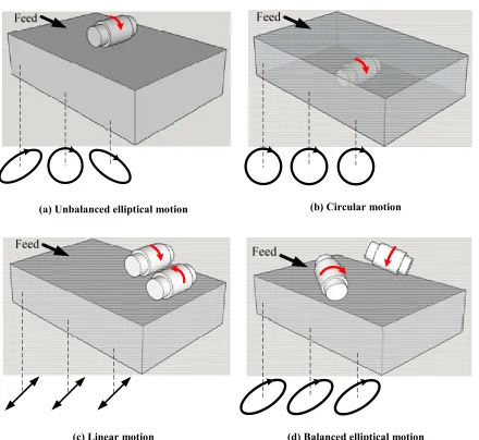
(a) Unbalanced elliptical motion (b) Circular motion

(c) Linear motion (d) Balanced elliptical motion

Figure 2-3: Shale shaker primary shapes of motion

end. However, the downward slope reduces fluid retention time and limits machine capacity. The next shale shaker generation, introduced in the late 1960s and early 1970s, produces a balanced circular motion, as illustrated in Figure 2-3(b). This type of motion can be achieved by placing a single rotating vibrator at the screen basket’s center of gravity. The consistent, circular vibration allows adequate solids transport with the screen basket in a horizontal orientation. Figure 2-3(c) illustrates a relatively new design that uses a pair of eccentric shafts rotating in opposite directions to produce linear screen basket motion. When placed at an angle to the screen basket, as shown in Figure 2-3(d), the eccentric shafts produce balanced elliptical motion. Linear and balanced elliptical motions provide superior separation and conveyance of cuttings, enabling inclined screens to provide improved liquid retention.

Shale shakers are traditionally designed and built for specific anticipated operating conditions. Factors that influence the associated vibration profile include the expected cutting types and mud flow rates. Because no one profile works efficiently across all drilling conditions, the shale shaker’s operating performance is thus fully specified at the design stage. Once the shale shaker is built, its vibration profile is neither tunable nor adaptable; any field operation that deviates from anticipated conditions results in sub-optimal shale shaker performance.

rotating forces; (2) accelerometers affixed to the shale shaker structure for measuring the vibration profiles, and (3) a controller that monitors these sensors and regulates actuator force magnitudes and phases to achieve and maintain a prescribed vibration profile. Figure 2-4 shows a schematic of the prescribed vibration system with three actuators mounted to the shale shaker. With appropriate actuator placement and sufficient force output, this system can be controlled to achieve all four of the primary vibration profiles of Figure 2-3. Additionally, progressive elliptical shape motion, illustrated in Figure 2-4, can be attained. This vibration profile enables superior cuttings conveyance and a staged processing of cuttings at the shale shaker entrance, middle and exit.

Figure 2-4: Prescribed vibration system with three actuators illustrating progressive elliptical motion as viewed from the side

vibration control solution for a well-posed problem has become practical, if not yet routine, given recent advances in control algorithms and microprocessors. However, the performance bottleneck for most systems involves poor compromise between performance and efficiency as a function of actuator placement. For simple systems, the designer can rely on intuition and experience in placing actuators, but more complex systems require multiple actuators whose optimal placement may defy intuition, and optimization of such systems by trial and error can be costly and time-consuming.

The presence of multiple attributes in an optimization problem, in principle, gives rise to a set of optimal solutions (known as Pareto-optimal solutions), instead of a single optimal solution. In the absence of any further information, none one of these Pareto-optimal solutions can be said to be better than the other. This demands a user to find as many Pareto-optimal solutions as possible [22]. The Pareto optimal solutions to a multi-attribute optimization problem often distribute regularly in both the decision space and the objective space. A problem that arises however is how to normalize, prioritize and weight the contributions of the various objectives in arriving at a suitable measure. In addition, these objectives can interact or conflict with each other in nonlinear ways. The present research seeks a more general method for optimizing the locations of multiple actuators in a shale shaker system with conflicting attributes.

of the chapter is organized as follows; in the next section, the prescribed vibration system dynamic models are derived, then marketing and optimization tools are combined with development of the preference-based multi-attribute optimization method based on conjoint analysis. Simulation and results are then presented, followed by conclusions and future work.

2.2

M

2.2.1

S

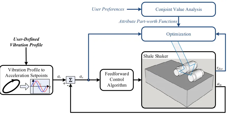
Figure 2-5 shows the control and optimization loops associated with the design of a prescribed vibration system (PVS). In the control loop, the user-specified vibration profile is converted to a time-domain reference acceleration , which is compared to the measured acceleration to determine the acceleration tracking error . A feedforward controller regulates the actuator control forces to minimize .

Vibration Profile to Acceleration Setpoints

t

y xA A,

( )t yk

&& ( )t xk && Feedforward Control Algorithm Shale Shaker

Conjoint Value Analysis

Σ Σ Σ Σ ar am τdist ae User-Defined Vibration Profile Optimization User Preferences

Attribute Part-worth Functions

+

The acceleration error also serves as the basis for the “performance” system attribute , a measure of how closely the measured vibration profile tracks the desired profiles for a specific vector of design parameters X. Another system attribute, the “efficiency” attribute , quantifies the power required to achieve a given performance. The optimization loop determines optimal actuator placement by minimizing an objective function, formulated using Conjoint Value Analysis (CVA). Details of the modeling, control and optimization methods are presented in subsequent sections.

2.2.2

V

P

D

The acceleration at location (where = 1, 2, 3 corresponds to the screen basket entrance, interior and exit, respectively) can be generalized by considering a typical elliptical vibration profile oriented at angle with major axis acceleration and minor acceleration , where is the ellipse ratio. Figure 2-6 illustrates the ellipse properties and the associated time history plots.

Based on the user-specified vibration profile, the x-axis and y-axis accelerations at location can be expressed as:

= cos + !

" = " cos# + !" $

(2.1) (2.2)

-8 -6 -4 -2 0 2 4 6 8 -8 -6 -4 -2 0 2 4 6 8 a

x (g's)

a y ( g 's ) m

A

0 0.2 0.4 0.6 0.8 1

-8 -6 -4 -2 0 2 4 6 8 Time (s) A c c e le ra ti o n ( g 's ) a x a y (b)

Figure 2-6: General vibration profile showing (a) x vs. y-axis elliptical vibration (b) x and y-axis

acceleration time histories

Using elliptical motion equations, the acceleration magnitudes are given by

= & sin + cos

(2.3)

" = &sin + cos

and the acceleration phases are given by

! = tan+ _⁄tan

(2.4)

!" = tan+ − tan⁄

Most vibration profiles under consideration are uniform where - , _" . = - , _" . =

- /, "/.. Thus, the designer needs to specify only the profile characteristics ( , , ) for

acceleration progression that correlates to the screen basket angular acceleration 1₂₃. The control problem can then be solved by considering the acceleration at location 1 and the angular acceleration, resulting in the reference vector = - , _" , 1₂₃.. Furthermore, the acceleration magnitudes and phases can be geometrically represented as a complex pair of static accelerations. Thus, the acceleration reference vector can be represented as follows

=

4 5 5 5 5 5 5

6 re# _:; $ im# _:; $ re# "_:; $ im# "_:; $ re# 1_{:;_23}$ im# 1:;_23$=>

> > > > > ?

(2.5)

2.2.3

S

B

V

M

x

y

y

ω

x

y

x y

ω,ni Fi,Φi

a

a

a

a

M,J

k

mi2

mi1

r

z

Figure 2-7: Screen basket outfitted with i actuators to create the desired vibration profile at measurement location k.

The CLM actuator produces the following forces and moments at the screen basket’s center of gravity

I = N Fcos − FOFsin P

FQ

I" = N F Fsin + OFcos P

FQ

@B = N −#GF− G23$R Fcos − FOFsin S P

FQ

+ #EF − E23$R F Fsin + OFcos S

(2.6)

For any steady-state vibration condition, the magnitudes and phases of the resultant forces and moments captured by (2.6) do not change. The only components of (2.6) that change are the time-dependent sin and cos terms. Thus, to simplify (2.6), the steady-state forces and moments can be expressed as functions of the static actuator force amplitudes and phases

IF and ΦF, respectively. The time-dependent trigonometric terms can be geometrically mapped

to the complex plane, where the cosine and sine terms are considered real and imaginary, respectively. The resulting model is a complex-valued matrix that quantifies the forces and moments at the screen basket center of gravity.

4 5 5 5 5

6_imIreI

reI" imI"

re@B

im@B=

> > > > ? = 4 5 5 5 5 5

6 1₀ 0_F

0 1

0

−#G − G23$ #E − E23$

#E − E23$ F #G − G23$ F

⋯ ⋯

1 0

0 F

0 1

F 0

−#GF− G23$ #EF− E23$

#EF− E23$ F #GF− G23$ F=>

> > > > ? W X Y X ZO ⋮ ⋮ F

OF\X

] X ^

(2.7)

Applying Newtonian mechanics to (2.7) yields a system model for the linear and angular accelerations at the screen basket center of gravity as functions of the actuator forces and screen basket properties. 4 5 5 5 5 5 5

6re# _23$ im# _23$ re# "_23$ im# "_23$ re# 123$ im# 123$ =

> > > > > > ? = 4 5 5 5 5 5

6 1 K⁄₀ 0

F⁄K

0 1 K⁄

0 −#G − G23$ A⁄B #E − E23$ A⁄B #E − E23$ F⁄AB #G − G23$ F⁄AB

⋯

1 K⁄ 0

0 F⁄K

0 1 K⁄

F 0

−#GF− G23$ A⁄B #EF− E23$ A⁄B #EF− E23$ F⁄AB #GF− G23$ F⁄ =AB>

> > > > ? W X Y X ZO ⋮ ⋮ F OF\X

] X ^

This model reflects that the screen basket response is a linear sum of the responses caused by each of the actuators. The net screen basket acceleration can be calculated based on the cross product of angular acceleration and offset distances of all actuators.

= 4 5 5 5 5 5 5

6re# _ $

im# _ $

re# "_ $ im# "_ $ re# 1₂₃$ im# 123$ =>

> > > > > ? = 4 5 5 5 5 5 5

6re# _23$ im# _23$ re# "_23$ im# "_23$ re# 123$ im# 123$ =

> > > > > > ? + 4 5 5 5 5 5

6re# 123$ × #G − G23$ im# 123$ × #G − G23$ re# 123$ × #E − E23$ im# 1₂₃$ × #E − E₂₃$

0

0 =>

> > > > ? (2.9)

In addition, (2.9) can be used to quantify the complex acceleration - _{"_} , _{"_} . at any measurement location using appropriate sensor location coordinates.

2.2.4

F

C

A

The feedforward controller, in this case a Least Mean Squares (LMS) adaptive algorithm [23], is used to minimize acceleration error . Although the LMS algorithm determines the actuator force amplitudes and phases (I_F and J_F) using the inverse of the system model (2.8), it is robust to the modeling errors associated with the dynamics of flexible structures. The LMS update law is

a = a − 1 + b∇d (2.10)

where a and a − 1 are the current and previous control outputs, b is the adaptation rate, and ∇_dis the instantaneous gradient estimate of the cost function with respect to I_F and

∇d= ef (2.11)

where ef is the conjugate transpose of the complex system matrix (2.8) and is the acceleration error vector at time step . Detailed derivations of the LMS algorithm can be found in [23], [24], [25], [26].

2.2.5

S

A

2.2.5.1 PERFORMANCE

The “performance” system attribute is defined to quantify system performance as a function of the design parameters . In this implementation, is the actuator location vector,

= DE , G , E , G … . EP, GPH, and is the mean square error of :

where h is the length of the acceleration error vector.

2.2.5.2 EFFICIENCY

A critical aspect of the PVS design process is accounting for the electrical power needed to drive the eccentric masses. Ideally, the system should be designed in a manner that minimizes required actuator power, which can be quantified in terms of motor torque i. This torque must account for gravitational forces, friction and damping effects, transient accelerations and disturbances associated with the motion of each actuator mounting base. During normal operating conditions, most of these torque components do not change

= j1_{h N} k

Q

significantly. However, the torque required to overcome base disturbances, hereinafter referred to as the disturbance torque i_lF:L, can vary in a way that significantly affects the total power requirement. For this reason, the “efficiency” system attribute is defined to be a scalar metric of i_lF:L.

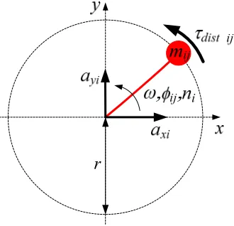
To facilitate the formulation of , consider one of the eccentric masses illustrated in Figure 2-8, part of the system shown in Figure 2-7. Eccentric mass K_Fm rotates in the x-y plane at a prescribed frequency with fixed radius r. The instantaneous angular position of K_Fm, defined relative to the x-axis, is given by _F + !_Fm, where !_Fm is the phase angle of the eccentric mass motion relative to the global coordinate system.

Figure 2-8: Mechanical schematic of an eccentric mass subjected to a disturbance base torque

The absolute motion of this eccentric mass can be determined directly from the system model (2.9). From the theory of forced vibration [27], the rotational center accelerations _F,

F = Fcos F + ! F

"F = "Fcos# F + !"F$

(2.13) (2.14)

where _F, _"F and ! _F, !_"F are the x and y-axis acceleration magnitude and phases respectively.

Using Figure 2-8, the disturbance torque i_{lF:L_Fm}can be expressed

ilF:L_Fm = nFm "Fopq# F + !Fm$ − nFm FqC # F + !Fm$ (2.15)

where n_Fm = K_Fm ∗ is the sLM mass imbalance of the CLMactuator.

Combining (2.13), (2.14) and (2.15), the disturbance torque expression becomes

ilF:L_Fm =1_{2 n}Fm- "Ftcos# F + !"F− F − !Fm$ + cos# F + !"F+ F + !Fm$u − Ftsin# F + ! F + F + !Fm$ − sin# F + ! F− F − !Fm$u.

(2.16)

which simplifies to

ilF:L_Fm =1_{2 n}Fm- "Ftcos#!"F− !Fm$ + cos#2 F + !"F+ !Fm$u − Ftsin#2 F + ! F + !Fm$ − sin#! F − !Fm$u.

(2.17)

(2.17) reveals that base motion creates a constant torque requirement i_{lF:L_l2_Fm}that depends on the base acceleration amplitudes _F and _"F and the relative phases #!_"F− !_Fm$ and#! _F − !_Fm$:

There is also a disturbance torque at the second harmonic of the angular rotation frequency:

ilF:L_v2_Fm =1_{2 n}Fm- "Fcos#2 + !"F+ !Fm$ − Fsin#2 + ! F + !Fm$.

(2.19)

Integrating this equation enables quantification of the alternating disturbance torque’s effects on eccentric mass speed and position:

lF:L_v2_Fm = −_{4A -}nFm "Fsin#2 + !"F+ !Fm$ + Fcos#2 + ! F+ !Fm$. + x (2.20) ylF:L_v2_Fm = −_{8A -}nFm "Fcos#2 + !"F+ !Fm$ − Fsin#2 + ! F+ !Fm$. + yx (2.21)

Because these effects are insignificant in comparison to the dc torque effect, they can be neglected, resulting in (2.18) being a sufficient representation of i_{lF:L_Fm}.

The efficiency attribute is defined to be the maximum absolute value of the individual eccentric mass disturbance torques:

= K Et{ilF:L_l2_ , … … . ilF:L_l2_Fm{u C = 1 … … , s = 1,2 (2.22)

At any steady-state condition, can be used to quantify the efficiency of the system.

2.2.6

M

-A

O

locations, however, affect the PVS attributes in a conflicting manner. In general, actuators can be located in a way that minimizes either or , but not both. This characteristic makes PVS design a nontrivial multi-attribute optimization problem where no single solution simultaneously optimizes both system attributes.

A well-optimized design requires an objective function that incorporates the relative importance of each attribute. In cases where the attributes are in conflict, subjective constraints or preferences need to be imposed. In order to optimize the prescribed vibration system, and need to be properly aggregated before any type of optimization technique is employed in the design process.

In general, multi-attribute design optimization involves finding the vector of design variables = DE , E , E_/… . E_PH that minimizes a set of attributes, or characteristics

= D , , / … . H

( )

X

f

( )

X

f

Dominated Solutions

Non-dominated Solutions Pareto Frontier

Figure 2-9: Pareto frontier in two-attribute problem

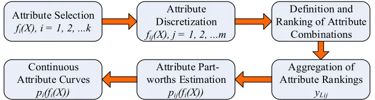
2.2.6.1 CONJOINT VALUE ANALYSIS

As illustrated in the flowchart of Figure 2-10, CVA starts with the selection of attributes

F , C = 1, 2, . . . that are most relevant to the design problem. For this research, the most

relevant attributes are the vibration tracking error and the system efficiency .

Attribute Selection

fi(X), i = 1, 2, ...k

Definition and Ranking of Attribute

Combinations Attribute

Discretization

fij(X), j = 1, 2, ...m

Aggregation of Attribute Rankings

yLij

Attribute Part-worths Estimation

pij(fi(X))

Continuous Attribute Curves

pi(fi(X))

Figure 2-10: Flow-chart for conjoint analysis

For each selected attribute, the expected range is discretized such that _Fm , s =

1, 2, . . . K, where K denotes the number of preferred levels. Different attribute combinations can be chosen to represent possible system performance features. It is not always practical to consider a full factorial set of attribute combinations as, in some cases, it can be cumbersome to define and sort the preferences. Thus, fractional factorial designs should be considered.

The next step is to rank the combinations so that the rankings reflect user or designer preferences. Several preference aggregation methods exist [31]; the choice of method depends on the nature of the rankings. This work employs the dummy-variable regression technique [32] to derive attribute part-worths, using ordinary least squares regression analysis. Part-worths are estimated by first normalizing the combination rankings G_~ using

G~ =_GG − G FP+ 1 v − G FP+ 2

where G is the ranking of each attribute combination and G _FP and G _v are the minimum and maximum rankings respectively. This normalized value is then used to calculate the logit coded ranking value, G_• using:

G• = h _{1 − G}G~ ~

(2.24)

This recoding performed for each ranking value and used to evaluate the subsequent regression problem. Logit coding [33] is a transformation of the rankings into scaled values that are appropriate for use with Ordinary Least Squares regression methods such as multiple regression. In cases where rankings are used to measure the designer’s preferences, logit recoding of the ranking values is required. This is because Ordinary Least Squares regression methods are not appropriate for conjoint data consisting of rank orders due to the difference between the representation of a rating and a ranking. In a rating, the data is scaled so that real differences in combinations are communicated by the arithmetic differences in their value. In other words, the difference between a rating of a 1 and 2 is the same as the difference between a rating of 9 and 10. In rankings, the same assumption cannot be true. For instance, a combination with a ranking of 4 is not necessarily twice as preferred as the combination ranked 2.

Finally, regression analysis is performed and the resulting coefficients are the attribute part-worths €_Fm that represent preferences for all the selected attribute levels. To normalize the part-worths, zero-centered transformation [32] can be applied to the regression analysis results.

optimization, continuous part-worth curves are needed, and can be obtained by piecewise linear interpolation and extrapolation of discrete part-worths curves. With the availability of continuous part-worths € # $, € # $, … . € for each attribute, the optimization problem is solved using an objective formulation that is based on part-worths.

2.2.6.2 OBJECTIVE FUNCTION FORMULATION

An objective function •# $ aggregates and combines attributes of interest into a simple, measurable quantity that the designer wishes to minimize. In this context, a given design variable yields an associated set of attributes _F , whose corresponding part-worth values €_F# _F $ are determined from the preference curves. In this implementation of CVA, the objective function is formulated as the negative sum of the attribute part-worths such that the optimization objective becomes minimization of this function as follows.

Minimize •# $ = − N €_F# _F $

FQ (2.25)

subject to _• ≤ ≤ _‚

2.2.6.3 SYSTEM OPTIMIZATION

Figure 2-11 shows a flow chart of the preference-based multi-attribute optimization scheme that has been developed by combining engineering and marketing tools.

Conjoint Value Analysis

SQP Optimization Marketing Tools

Engineering Tools

System Dynamic Model User Preferences

User-Defined Vibration Profiles

Attribute Part-worth Functions

Optimized Actuator Locations

Figure 2-11: Multi-attribute optimization based on conjoint analysis

The system model provides the attributes and as functions of the actuator locations. Conjoint analysis provides preference-based attribute part-worths as functions of the system attributes. At each optimization step, the optimization routine determines the instantaneous part-worths associated with a specific design then uses the objective function defined in (2.25) to adapt the actuator locations. The actuator location space must be constrained such that there can be no overlap between the spaces occupied by the actuators.

the step size . The new point in the design space is obtained as E _„ = ƒ . In this method, the direction vector, ƒ is obtained by solving the QP sub-problem, shown below.

Minimize 1

2 ƒ…ƒ + ∇ …ƒ

Subject to ∇•_F…ƒ + •_F…ƒ ≤ 0

∇ℎ_F…_{ƒ + •}

F…ƒ ≤ 0 E• _{≤ ƒ + E ≤ E}‚

(2.26)

where ƒ is the design variable. ∇ , ∇• and ∇ℎ are the gradients of the objective, inequality constraints and equality constraints respectively. Thus ƒ , the direction vector, is obtained. Step size, is chosen equal to 0.5ˆ where A is the first of the integers ‰ = 1,2,3 … for which the following inequality holds:

y E + 0.5Š_{ƒ ≤ y E − ‹0.5}Š_{‖ƒ‖ (2.27)}

where y E can be used as a descent function. Further details of the method can be seen in [5] and [35].

2.2.7

S

Table 2-1: PVS physical parameters

2.2.7.1 CASE 1:OPTIMIZING AN ACTUATOR GROUP LOCATION The optimization problem was formulated as follows:

Minimize •# $ = −t€ # $ + € # $u

•≤ ≤ ‚

where € is the part-worth associated the vibration tracking error and € is the part-worth associated with the system efficiency . The design constraints _• and _‚ were defined as offsets from the initial location vector _x and they were specified as

•• = D •‚ = D

−1.000 −0.250 −1.000 −0.250 −1.000 −0.250

0.200 0.100 0.200 0.100 0.200 0.100

H H

K K

Parameter Value Description

Ž 2000 KK Screen basket length

@ 2430 • Screen basket mass

AB 140 • ∙ K Screen basket Inertia

K_• 130 • Actuator mass

A• 1.2 • ∙ K Actuator inertia

232.48 ∙ ƒq+ _{Vibration angular velocity}

n 0.675 • ∙ K Eccentric mass imbalance

-E23, G23. D1090, 535HKK Screen basket CG location

DE , G H D2000,350H KK Measurement location 1

DE , G H D1000,350H KK Measurement location 2

DE /, G /H D0, 350H KK Measurement location 3

3 Number of actuators

D , , /H D−1,1, −1H Actuator rotational direction

In addition, the actuator locations were fixed relative to each other, such that the solution represented as a pair of E and G-axis deviations from _x.

Discretized levels for and were selected as shown in Table 2-2.

Table 2-2: Discretized levels for f1(X) and f2(X)

”• • (G’s) # ”_– • (Nm)

1 0.0 5 10

2 0.25 6 20

3 0.50 7 25

4 1.0 8 30

Preferences were selected as shown in Table 2-3, where the highest rank number reflects the most preferred attribute combination.

Table 2-3: Preferences for attribute combinations

Rank Combination Rank Combination

16 1,5 8 3,6

15 1,6 7 4,5

14 1,7 6 2,8

13 2,5 5 3,7

12 2,6 4 4,6

11 1,8 3 3,8

10 2,7 2 4,7

9 3,5 1 4,8

Table 2-4: Discrete Part-worths obtained for each level

”• • (G) Part-worth ”_– • (Nm) Part-worth

0.0 53.4307 10 91.2006

0.25 23.7251 20 20.9686

0.50 -13.8306 25 -20.1257

1.0 -63.3252 30 -92.0435

Figure 2-12 shows and preference curves that are piecewise linearly interpolated and extrapolated and to obtain continuous part worth for every design case.

(a) (b)

Figure 2-12: Preference curves for (a) f1(X) and (b) f2(X)

2.2.7.2 CASE 2:OPTIMIZING INDIVIDUAL ACTUATOR LOCATIONS The design optimization case was configured as follows:

Minimize •# $ = −t€ # $ + € # $u

•≤ ≤ ‚

0 0.2 0.4 0.6 0.8 1

-80 -60 -40 -20 0 20 40 60

Vibration Error, f₁(X) (G's)

P ar tw o rt h

0 10 20 30

-100 -50 0 50 100

Torque Disturbance, f₂(X) (Nm)

Where the design constraints _• and _‚ were defined as offsets from the initial location vector _x and the specified as

•• •‚

= D

= D

−1.500 −0.250 −1.500 −0.250 −1.500 −0.250

0.250 0.100 0.250 0.100 0.250 0.100

H

H K K

In this case, the actuator locations were optimized individually, with no constraint keeping them at fixed relative locations. However, the optimization was configured to eliminate solutions with actuator space overlap.

The levels for and were discretized as shown in Table 2-5.

Table 2-5: Discretized levels for f1(X) and f2(X)

# ”_• • (G’s) # ”_– • (Nm)

1 0.0 5 0

2 0.25 6 10

3 0.50 7 20

4 1.0 8 30

Table 2-6: Preferences for attribute combinations

Combination Combination

Rank Preference 1 Preference 2 Rank Preference1 Preference 2

16 1,5 1,5 8 3,5 2,7

15 1,6 2,5 7 3,6 1,8

14 1,7 3,5 6 3,7 4,6

13 1,8 1,6 5 3.8 3,7

12 2,5 2,6 4 4,5 2,8

11 2,6 3,6 3 4,6 4,7

10 2,7 4,5 2 4,7 3,8

9 2,8 1,7 1 4,8 4,8

Figure 2-13 shows the resulting and preference curves that are piecewise linearly interpolated and extrapolated and to obtain continuous part worth for every design case.

(a) (b)

Figure 2-13: Preference curves for (a) f1(X) and (b) f2(X)

0 0.2 0.4 0.6 0.8 1

-150 -100 -50 0 50 100 150

Vibration Error, f

1(X) (G's)

P a rt w o rt h Preference 1 Preference 2

0 10 20 30

-100 -50 0 50 100

Torque Disturbance, f

2(X) (Nm)

2.3

R

2.3.1

C

1:

O

A

A

G

L

Figure 2-14 shows the vibration performance of the initial, non-optimized system with

= x and = 19.3Nm. for Profile 1.

(a)

(b) (c)

Figure 2-14: X0 design performance for a progressive profile at locations (a) 1, (b) 2 and (c) 3

-5 0 5

-5 0 5

x-axis Acceleration (G's)

y-a x is A c c e le ra ti o n ( G 's ) Desired Measured

-5 0 5

-5 0 5

x-axis Acceleration (G's)

y-a x is A c c e le ra ti o n ( G 's ) Desired Measured

-5 0 5

-5 0 5

x-axis Acceleration (G's)

Figure 2-15 shows the convergence of the objective function •# $ and the offset of the actuator location vector from the initial location vector x during the optimization.

(a)

(b)

Figure 2-15: Convergence of the (a) objective function and (b) location vector offset from X0

0 20 40 60 80 100 120

-150 -100 -50 0 50 Iteration Number g( f( X))

0 20 40 60 80 100 120

0 50 100 150 200 250 Iteration Number x-a x is o ff se t fr o m X

o (

m

m

)

0 20 40 60 80 100 120-250

-200 -150 -100 -50 0 y-a x is o ff se t fr o m X

o (

m

m

)

x-axis offset

Figure 2-16 shows the screen basket vibration performance for profile 1, based on the optimized actuator location vector whose offsets from _x are ∆E = 59 KK and ∆G =

−214 KK, with = 4.2˜K.

(a)

(b) (c)

Figure 2-16: Optimized performance for a progressive profile at locations (a) 1, (b) 2 and (c) 3

-5 0 5

-5 0 5

x-axis Acceleration (G's)

y-a x is A c c e le ra ti o n ( G 's ) Desired Measured

-5 0 5

-5 0 5

x-axis Acceleration (G's)

y-a x is A c c e le ra ti o n ( G 's ) Desired Measured

-5 0 5

-5 0 5

x-axis Acceleration (G's)

Tables -7 and -8 show the initial and optimized system performance across five vibration profiles. This performance yields significant reductions in both and .

Table 2-7: f1(X) initial and optimized performance across five vibration profiles

Profile ”_• • (G’s)

Initial Optimized Percent Improvement (%)

1 0.65 0.16 75.4

2 0.82 0.78 4.9

3 0.49 0.22 55.1

4 0.24 0.09 62.5

5 1.22 1.03 15.6

Table 2-8: f2(X) initial and optimized performance across five vibration profiles

Profile ”_– • (Nm)

Initial Optimized Percent Improvement (%)

1 19.3 4.2 78.2

2 26.0 20.0 23.1

3 28.8 17.0 41.0

4 19.0 13.0 31.6

5 24.0 13.0 45.8

(a) (b)

Figure 2-17: Percentage Improvement over initial system design for (a) f1(X)and (b) f2(X)

2.3.2

C

2:

O

I

A

L

The respective solutions • and • based on preferences 1 and 2 were

•

• = D = D

0.200 −0.250 0.060 −0.250 −0.162 −0.250H

0.200 −0.250 0.200 −0.090 0.200 −0.161H

K

K

where • and • are the design parameter offsets relative to the initial design point •_x. As seen in the vectors, most of the actuator location changes saturated at the constraint boundaries.

Figure 2-18 shows the vibration performance based on the optimized actuator locations that resulted from the two different preferences.

1 2 3 4 5

0 10 20 30 40 50 60 70 80 Profile Identifier % I m p ro v e m e n t in

f(1 X)

1 2 3 4 5

0 10 20 30 40 50 60 70 80 Profile Identifier % I m p ro v e m e n t in

f(2 X)

(%

(a)

(b) (c)

Figure 2-18: Optimized performance for a progressive profile at locations (a) 1, (b) 2 and (c) 3

Tables -9 and -10 show initial and optimized system performance across five vibration profiles. Both preferences show a significant reduction in and .

-5 0 5

-5 0 5

x-axis Acceleration (G's)

y-a x is A c c e le ra ti o n ( G 's ) Desired Preference 1 Preference 2

-5 0 5

-5 0 5

x-axis Acceleration (G's)

y-a x is A c c e le ra ti o n ( G 's ) Desired Preference 1 Preference 2

-5 0 5

-5 0 5

x-axis Acceleration (G's)

Table 2-9: f1(X) initial and optimized performance across five vibration profiles

Profile ”_• • (G’s)

Initial Optimized Percent Improvement (%)

Preference 1 Preference 2 Preference 1 Preference 2

1 0.65 0.13 0.17 80.8 74.3

2 0.82 0.79 0.79 4.3 4.1

3 0.49 0.22 0.29 55.1 41.0

4 0.24 0.12 0.18 51.2 24.4

5 1.22 0.86 0.85 29.7 31.6

Table 2-10: f2(X) initial and optimized performance across the five vibration profiles

Profile ”_– • (Nm)

Initial Optimized Percent Improvement (%)

Preference 1 Preference 2 Preference 1 Preference 2

1 19.3 9.24 5.59 52.1 71.0

2 26.0 21.03 25.07 19.2 3.7

3 28.8 18.05 19.44 37.4 32.6

4 19.0 13.36 14.40 30.4 24.9

5 24.0 16.46 13.97 32.7 42.9

Figure 2-19 shows a graphical representation the improved performance across five vibration profiles.

(a) (b)

Figure 2-19: Percentage improvement of over initial system design for (a) f1(X) (b) f2(X)

1 2 3 4 5

0 20 40 60 80 100 Profile Identifier % I m p ro v e m e n t in

f( 1

X) Preference 1

Preference 2

1 2 3 4 5

0 20 40 60 80 Profile Identifier % I m p ro v e m e n t in

f( 2

X)

(%

)

In all cases, the optimized solutions both perform better than the nominal configurations. There is a slight performance difference between the two solutions caused by the effect of the preference rankings.

2.4

C

This chapter details a novel design optimization strategy for a prescribed vibration system (PVS) used to mechanically filter solids from fluids in oil and gas drilling operations. Conjoint value analysis (CVA), a statistical technique commonly used in marketing science, was employed to incorporate designer preferences. This approach effectively quantified and optimized preference-based trade-offs in the design process, and yielded performance improvements in all system attributes across all simulated vibration profiles.

The initial design configuration (an open-loop prototype built before these optimization tools were developed), represented by the design vector _x, was used as a benchmark for performance and efficiency comparisons. In the first design case, five equally spaced levels of attribute ranges were used in discretization, though non-uniform spacing could be used to change the resolution in critical ranges. In the second case, most of the actuator location changes saturated at the constraint boundaries. Preference 1 caused the location changes to saturate along the y-axis while Preference 2 resulted in saturation in the x direction. While the solutions provide good trade-offs between the two attributes, it is also an indication that performance could be further improved if the design space were expanded.

CHAPTER

3:

UNCERTAINTY

AND

SENSITIVITY

ANALYSIS

OF

PRESCRIBED

VIBRATION

SYSTEM

DESIGNS

3.1

I

Technological advances that introduce increased system complexity can add significant uncertainty to design parameters, boundary conditions and system behavior. The Prescribed Vibration System presented in Chapter 3 is one such example and provides the basis for the work presented in this chapter. Sources of uncertainty in this system include manufacturing variations, design imprecision, errors in inertial approximations and structural irregularities. While there are ways to quantify and reduce these errors, they are impossible to eliminate entirely. Design decisions still have to be made in the face of risky and uncertain system performance. The realization that decision making is an intricate part of engineering design has inspired research in solution space exploration [9], data variability [10], decision analysis and multi-attribute decision making [3] [4]. The main goal of a decision-making process is improving decision quality and creating reliable and profitable products [11]. Techniques that incorporate designer preferences coupled with uncertainty studies can be used in product development to help accomplish this goal.

a probabilistic approach, which assumes known probability density function (pdf) information. The benefit of probabilistic analysis is the ability to produce comprehensive results, versus a single result based on the mean design point. These probabilistic techniques have been successfully used in many applications such as bridge failure assessment, multi-criteria decision analysis and reliability of steel connections [12], [13], [14]. In addition, it has been shown that incorporating uncertainty-based analysis and/or reliability-based design can provide risk reduction by accounting for various uncertainties in the design process [15]. It is, therefore, essential for the overall design choice to be based not only on the performance objectives but also on the resulting system robustness. This is valuable, considering the uncertainties that can result from manufacturing variations and tolerance stacks.

The remainder of the chapter is organized as follows: the next section presents the reformulation of the design vector and the system attributes. It then examines Monte Carlo-based uncertainty and sensitivity analyses as a way to quantify the relative robustness of alternative designs to design parameter imprecision. Simulation and results are then presented, followed by conclusions and future work.

3.2

M

3.2.1

D

V

R

The system design vector ™ can be reformulated as

™ = DE , G , E , G … . EP, GP, nH (3.1)

where, E , G , E , G … . E_P, G_P is the actuator location vector , described in Chapter 2; n is the product of the actuator eccentric mass m and the fixed rotation radius r and it defines the actuator force capacity. Adding the actuator force capacity to the design vector provides an additional degree of freedom in the system design.

3.2.2

S

A

R

For any desired acceleration profile, the goal is to minimize the vibration magnitude error and the vibration angle error in a manner that minimizes required actuator power. Referring to the generic elliptical profile shown in Figure 2-6(a), the difference between | and

magnitude error |›|. The difference between | and | , the respective reference and measured major axis angles, defines the vibration angle error ›_∠.

|›| = | _•− | _•

›∠ = | _ − | _

= 1, 2, 3 (3.2)

3.2.2.1 PERFORMANCE

The reformulated “performance” system attributes ž # ™$ and ž # ™$ are defined to quantify system performance as a function of the design parameters ™. In this implementation, ž # ™$ is the mean square error of the magnitude error |›| and ž # ™$ is the mean angle error ›_∠ across the three shale shaker locations of interest.

Decoupling the performance attributes that relate to the magnitude and angle of the vibration error gives the designer flexibility in the design process. As an example, the designer can choose to give up angle tracking performance to gain magnitude tracking, if magnitude is deemed be more important.

3.2.2.2 EFFICIENCY

The reformulated efficiency attribute ž_/# ™$ is the maximum value of the squared disturbance torques:

ž # ™$ = Ÿ1_{3 N |›|}/

Q (3.3)

ž # ™$ = 1_{3 N}/ ›_∠

ž_{/# ™$ = K E ilF:L¡¢££ , … … . ilF:L}

¡¢¤¥ ¦ ; C = 1. . ; s = 1,2 (3.5)

In contrast to the efficiency attribute described in (2.22), ž_/# ™$ represents a quantity proportional to the square of the current, a measure that is more representative of the power required to drive the eccentric masses.

3.2.3

U

S

A

The Monte Carlo method [37] of performing uncertainty and sensitivity analyses selects a random set of design parameter values drawn from their individual probability distributions. These values are then used in the simulation model to obtain corresponding system output values. This process is repeated many times, each time making sure the output is valid for the chosen parameter values. The result is a probability distribution of system attributes that result from design parameters variations.

3.2.3.1 UNCERTAINTY ANALYSIS

Uncertainty [38] involves the notion of randomness. If a performance measure varies, and this variation over space and time cannot be predicted with certainty, it is called a random variable. One cannot say with certainty what the value of a random variable will be, but only the likelihood or probability that it will be within some specified range. An uncertainty analysis takes a set of randomly chosen design parameter values and evaluates distributions (or statistical measures) of the resulting outputs [37], [38].

As illustrated in Figure 3-1, the Monte Carlo-based uncertainty analysis involves the following four steps:

1. Design parameter range and distribution selection - if the analysis is exploratory, rough distribution assumptions may be adequate. In this research, the design vector elements are assigned a normal probability distribution. The normal distribution is chosen because it maximizes the information entropy among all distributions with a known mean and standard deviation [39]. The standard deviations were obtained from statistical data gathered by a shale shaker manufacturer. The data quantifies the previously observed standard deviations of actuator locations as a result of design and manufacturing imprecision.