Robust Gossip Based Communication Using GD Clustering Algorithm

(1)

ISSN(Online): 2320-9801

ISSN (Print) : 2320-9798

I

nternational

J

ournal of

I

nnovative

R

esearch in

C

omputer

and

C

ommunication

E

ngineering

(An ISO 3297: 2007 Certified Organization)

Vol. 4, Issue 3, March 2016

Robust Gossip Based Communication Using

GD Clustering Algorithm

A.Vikram1, R.Sinduja2*, S.Vinothini2, A.Shivapriya2, S.Nalini2

Assistant Professor, Department of Computer Science and Engineering, Saranathan College of Engineering, Trichy,

Tamil Nadu, India1

IV B.E. Students, Department of Computer Science and Engineering, Saranathan College of Engineering, Trichy,

Tamil Nadu, India2

ABSTRACT: Gossip is a simple communications which assumes no predefined structure in the networks. General Decentralized cluster dataset is circulated among large no of nodes in a distributed environment. It handles two types clustering partition-based, density-based while being fully decentralized, asynchronous and also adaptable to churn. In existing method a distributed clustering algorithm, our algorithm does not require a central site to coordinate execution rounds, and/or merge local models. It avoids global message flooding. RACHET is a hierarchical clustering algorithm in which, each site executes the clustering algorithm locally, and transmits a set of statistics to a central site. It based on the peer to peer networks.

KEYWORDS: Partition based clustering, Density based clustering, General decentralized clustering, RACHET, Algorithm.

I. INTRODUCTION

Clustering, or unsupervised learning, is important for analyzing large data sets. Clustering are the partitions of data into groups (clusters) of similar objects, with high intra-cluster similarity and low inter-cluster similarity. With the progress of large-scale distributed systems, huge amounts of data are increasingly originating from dispersed sources. Analyzing this data, using centralized processing, is often infeasible due to communication, storage and computation overheads. Distributed Data Mining (DDM) focuses on the adaptation of data-mining algorithms for distributed computing environments, and intends to derive a global model which presents the characteristics of a data set distributed across many nodes.

In fully distributed clustering algorithms, the data set as a whole remains dispersed, and the participating distributed processes will gradually discover various clusters. Communication complexity and overhead, accuracy of the derived model, and data privacy are among the concerns of DDM. Typical applications requiring distributed clustering include: clustering different media metadata (documents) from different machines; clustering nodes’ activity history data (devoted resources, issued queries; download and upload amount, etc.); clustering books in a distributed network of libraries; clustering scientific achievements from different institutions and publishers.

A common approach in distributed clustering is to combine and merge local representations in a central node, or aggregate of local models in a hierarchical structure Some recent proposals, although being completely decentralized, include synchronization at the end of each round, and/or require nodes to maintain history of the clustering.

In this paper, a General Distributed Clustering algorithm (GD Cluster) is proposed and instantiated with two popular partition based and density-based clustering methods. We first introduce a basic method in which nodes gradually build a summarized view of the data set by continuously exchanging information on data items using gossip-based communication. Gossiping is used as a simple, robust and efficient dissemination technique, which assumes no predefined structure in the network. The summarized view is a basis for executing weighted versions of the clustering algorithms to produce approximations of the final clustering results.

(2)

ISSN(Online): 2320-9801

ISSN (Print) : 2320-9798

I

nternational

J

ournal of

I

nnovative

R

esearch in

C

omputer

and

C

ommunication

E

ngineering

allow customization for other classes of clustering, which are left out of the current paper. We also discuss enhancements to the algorithm particularly aimed at improving communication costs.

The simulation results presented using real and synthetic data set, show that GD Cluster is able to achieve a high-quality global clustering solution, which approximates centralized clustering. We also explain effects of various parameters on the accuracy and overhead of the algorithm. We compare our proposal with central clustering and with the LSP2P algorithm and also show its supremacy in achieving higher quality clusters. The main contributions of this paper are as follows:

 Proposing a new fully distributed clustering algorithm, can be instantiated to at least two categories of clustering algorithms.

 Dealing with dynamic data and evolving the clustering model.

 Empowering nodes to construct a summarized view of the data, to be able to execute a customized clustering algorithm independently.

 Efficiently searching the content of the documents.

 Analyze the performance of searching.

This paper is organized as follows. The system model is described in Section 2. In Section 3, the basic decentralized algorithm is introduced. In the succeeding section we propose adjustments to deal with churn. Section 5 discusses enhancements. Simulation results are discussed in Section 6, followed by related work and conclusion.

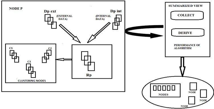
Fig. 1. A graphical view of the system model.

II. RELATED WORK

Distributed data mining is a dynamically growing area. A discussion and comparison of several distributed centroid based partition clustering algorithms is proposed in parallel K-means clustering, by first distributing data to multiple processors. In each synchronized algorithm round, every processor broadcasts its currently obtained centroids, and updates the centroids based on the information received from all other processors. Different from many existing distributed clustering algorithms, our algorithm does not require a central site to coordinate execution rounds, and/or merge local models. Also, it avoids global message flooding. RACHET [5] is a hierarchical clustering algorithm in which, each site executes the clustering algorithm locally, and transmits a set of statistics to a central site.

(3)

ISSN(Online): 2320-9801

ISSN (Print) : 2320-9798

I

nternational

J

ournal of

I

nnovative

R

esearch in

C

omputer

and

C

ommunication

E

ngineering

high dimensional feature vectors is presented in [9], which uses a central site to build the global model. SDBDC [2] is a distributed density-based clustering algorithm that summarizes local statistics, and transmits them to a central site to be merged. Aouad et al. [10] propose a lightweight distributed clustering technique based on merging of independent local sub clusters according to an increasing variance constraint. Merugu and Ghosh [11] propose a distributed clustering algorithm, in which each node computes a probabilistic clustering model and a central node attempts to aggregate the local models in to reduce an approximate cost function. Some distributed clustering proposals impose a special structure in the network. A hierarchical clustering method based on K-means for P2P networks is suggested in [1]. Summary representations are then transferred up the hierarchy and merged to obtain k global clusters. Lodi et al. Embeddings of kernel clustering on the Map Reduce framework is proposed in [12]. Some solutions which consider pure unstructured networks, require state-aware operation of nodes, work in static settings, or are aimed at computing basic functions like average and sum. Fellus et al. proposed a decentralized K-means algorithm which executes in iterations, and in each iteration nodes compute an approximation of the new centroids in a distributed manner. Datta et al. Eyal et al. [13] provide a generic algorithm for clustering in a static network. Fatta et al. [14] propose a gossip-based distributed k-means clustering, which is initiated with similar initial centroids, and proceeds towards centroid convergence with rounds of gossiping. Shen and Li [15] propose a distributed clustering in a static network, incorporating information theory measures. The major drawback of the majority of existing approaches is the lack of efficient solutions for adaptability in dynamic settings, which introduces significant challenges for applying the algorithms in large-scale real-world networks. Also, majority of approaches limit nodes to finding the same number of clusters.

III. SYSTEM MODEL

We consider a set P={p1, p2, . . . , pn} of n networked nodes. Each node p stores and shares a set of data items Dp int , denoted as its internal data, which may change over time. D = Up∈pDp int is the set of all data Items available in the network. Each data item d is presented using an attribute (meta data) vector denoted as Each data item d is presented using an attribute (meta data) vector denoted as dattr. Whenever transmission of data items is mentioned in the text, transmission of the respective attribute vector is intended. While discovering clusters, p may also store attribute vectors of data items from other nodes. These items are referred to as the external data of p, and denoted as Dp ext . The union of internal and external data items of p is referred to as Dp = Dp int ∪Dp ext.

During algorithm execution, each node p gradually builds a summarized view of D, by maintaining representatives, denoted as Rp = {r1p , r2p , . . . , rkpp}. Each representative r ∈ Rp is an artificial data item, summarizing a subset Dr of

D. The attribute vector of r, rattr, is ideally the average of attribute vectors1 of data items in Dr. The intersection of these

subsets need not be empty, i.e., ∀r, r′ Rp. |Dr ∩Dr | ≥ 0. The actual set Dr is not maintained by the algorithm, and is ∈ discarded once r is produced. Each data item or representative x in p, has an associated weight Wp(x). The weight of x is equal to the number of data items which, p believes, x is composed of. Depending on whether x is a representative or a data item, Wp(x) should ideally be equal to |Dx| or one, respectively. The goal of this work is to make sure that the complete data set is clustered in a fully decentralized fashion, such that each node p obtains an accurate clustering model, without collecting the whole data set. The representation of the clustering model depends on the particular clustering method. For partition based and density based clustering, a centroid and a set of core points can serve as cluster indicators, respectively. Whenever the actual type of clustering is not important, we refer to the clustering method simply as F. Fig. 1 provides a summarized view of the system model.

IV.DECENTRALIZED CLUSTERING

Each node gradually builds a summarized view of D, on which it can execute the clustering algorithm F. In the next subsections, we first discuss how the summarized view is built. Afterwards, the method of weight calculation is described, followed by the execution procedure of the clustering algorithm.

A. Building The Summarized View:

(4)

ISSN(Online): 2320-9801

ISSN (Print) : 2320-9798

I

nternational

J

ournal of

I

nnovative

R

esearch in

C

omputer

and

C

ommunication

E

ngineering

for part of the data set located near Dint p . For other parts, it solely collects representatives. Accordingly, it gradually builds a global view of D. Each node continuously performs two tasks in parallel:

i) Representative derivation, which we name DERIVE and ii) representative collection, which we name COLLECT. The two tasks can execute repeatedly and continuously in parallel. An outline of the tasks performed by each node is demonstrated in We use two gossip-based, decentralized cyclic algorithms to accomplish the two tasks, as described in the next subsections.

A1. Derive

To derive representatives for part of the data set located near Dp int, p should have an accurate and up-to-date view of the data located around each data d∈Dp int . In each round of the DERIVE task, each node p selects another node q for a three-way information exchange, It should first send Dp int to another node. If size of Dint p is large, it can summarize the internal data by an arbitrary method such as grouping the data using clustering, and sending one data from each group. Node p then receives from q, data items located in radius r of each d ∈ Dp int , based on a distance function d . r is a user-defined threshold, which can be adjusted as p continues to discover data. In the same manner, it will also send to q the data in Dp that lie within the r radius of data in another node. The operation update Local Data() is used to add the received data to Dp ext .Knowing some data located within radius r of some internal data item d, node p can summarize all this data into one representative. This is performed periodically by rounding t gossip using the algorithm of merge weights function which updates the representative weight, and is later described in detail.

A2. Collect

To fulfill the COLLECT task, each node p selects a random node every T time units, to exchange their set of representatives with each other . Both nodes store the full set of representatives. The summarize function used in the algorithm, simply returns all the representatives given to it as input. A special implementation of this function is described in Section 5.1, which reduces the number of representatives.

Initially, each node has only a set of internal data items, Dp int .Thus, the set of representatives at each node is initialized with allof its data items, i.e., Rp = Dp int.The two algorithms of tasks DERIVE and COLLECT, startwith a preprocessing operation. In this basic algorithm, these operations have no special function, thus we defer their discussion to Section 4. The graphical representation of the communicationperformed in DERIVE and COLLECT is depicted inthe operation selectNode() employsa peer-sampling service to return a node selected uniformly atrandom from all live nodes in the system .

B. Weight Calculation:

When representatives are merged, for example in the function remove Representatives, a special method should be devised for weight calculation. The algorithm does not record the set Dr for each representative r, due to resource constraints.

Also, there is a possibility of intersection between summarized data of different representatives. To address the weight calculation issue, representative points are accompanied by a (small size) “estimation field”, that allows us to approximate the number of actual items it represents.

(5)

ISSN(Online): 2320-9801

ISSN (Print) : 2320-9798

I

nternational

J

ournal of

I

nnovative

R

esearch in

C

omputer

and

C

ommunication

E

ngineering

Fig.2. A schematic diagram of Weight Calculation

C. Final clustering:

The final clustering algorithm F is executed on the set of representatives in a node. Node p can execute a weighted version of the clustering algorithm on Rp, any time it desires, to achieve the final clustering result. In a static setting, continuous execution of DERIVE and COLLECT will improve the quality of representatives causing the clustering accuracy to converge. In the following, we discuss partition-based and density-based clustering algorithms as examples.

C1. Partition-based clustering

K-means [12] considers data items to be placed in an m-dimensional metric space, with an associated distance measure d. It partitions the data set into k clusters, C1,C2, . . . , Ck. Each cluster Cj has a centroid mj, which is defined as the average of all data assigned to that cluster. This algorithm tries to minimize the following objective function:

K

∑ ∑|| dl-µj ||2 eq. (1)

J=1 dl€ cj

Weighted K-means assumes a positive weight for each data item and uses weighted averaging. They themselves will be assigned weight values, indicating number of data assigned to the clusters. The formal definition of the weighted K-means is given in detail.

The algorithm proceeds heuristically. A set of random centroids are picked initially, to be optimized in later iterations. The available approaches of distributed partition-based clustering typically assume identical initial K-means centroids in all nodes [4], [5], [6]. This is, however, not required in our algorithm as each node can use an arbitrary parameter k with an arbitrary set of initial centroids.

C2. Density-Based Clustering

In density-based clustering, a node p can execute, for example, a weighted version of DBSCAN on Rp with parameters minPts and ". In DBSCAN, a data item is marked as a core point if it has at least minPts data items within its radius. Also, two core points are within one cluster, if they are in “range of each other, or are connected by a chain of core points, where each two consecutive core points have a maximum distance of “. A non-core data item located within distance from a core point, is in the same cluster as that core point, otherwise it is an outlier.

In our algorithm, each representative may cover a region with radius 2 greater than. Also a representative does not necessarily have the same attribute vector as any regular data item. Therefore, representatives do not directly mimic core points. Nevertheless, core points in DBSCAN are a means of describing data density. Adhering to this concept, representatives can also indicate dense areas.

The ᵖ parameter of the DERIVE task can be set to €. This ensures that if some data item is a core point, the

(6)

ISSN(Online): 2320-9801

ISSN (Print) : 2320-9798

I

nternational

J

ournal of

I

nnovative

R

esearch in

C

omputer

and

C

ommunication

E

ngineering

In GoScan nodes detect core points and disseminate them through methods very similar to COLLECT and DERIVE. GoScan is an exact method, whereas here we are providing an approximate method. The approximation imposes less communication overhead, and faster convergence of the algorithm.

D. Dynamic Data Set:

Real-world distributed systems change continuously, because of nodes joining and leaving the system, or because Their set of internal data is modified. To model staleness of data, each data item will have an associated age. Agep(d) denotes the time that node p believes has passed since d was obtained from its originating, owning node. Time is measured in terms of gossiped rounds. The age of data items accompany them in the DERIVE task. The age of an external data item at node p is increased (by p) before each communication; the age of an internal data always remains zero to reflect that it is stored (and upto-date) at its owner. If a node p receives a copy d0 of a data item d it already stores, age p(d) is set to min{age p(d),age p(d’)} (and d’is further ignored).

When a data item d is removed from the original peer, the minimal recorded age among all its copies will only increase. Node p can remove data item d if age p(d) > MaxAge, where MaxAge is some threshold value, presuming that the original data item has been removed. An age argument is also associated with each representative; age p(r) is set to zero when r is first produced by p, and increased by one before each communication.

The weight of a data item or a representative is a function of its age. For a data item d, the weight function is ideally one for all age values not greater than MaxAge. The data items summarized by a representative have different lifetimes according to their age. Therefore, the weight of the representative should capture the number of data items summarized by the representative at each age value. When the weight value falls to zero, the representative can be safely removed. We will see below that instead of the actual weight, the weight estimators are stored per each age value to enable further merging and updating of representatives.

The weight function of a representative will always be in the form of a descending step function for values greater than age p(r), and will reach zero at most at age p(r)+ MaxAge. All of the data currently embedded in the representative will be gradually removed, and no data can last longer that MaxAge units from the current time.

With the weight function being dependent on age, the weight estimators are in turn bound to the age values. ^wpl(x, t) presents the l’th weight estimator of item x in age t, from the view of peer p. For a data item d, while age p(d) ≤

MaxAge, each weight estimator preserves its initial value, and is null otherwise. For a representative r, s weight estimators are recorded at each age value greater than age p(d), up to the point where all data embedded in the representative are removed. To incorporate these new concepts in the basic algorithm, the two preprocessing operations of DERIVE and COLLECT should be modified to increase age values of data and representatives, and remove them if necessary. Moreover, before storing the received data in DERIVE, the age values for repetitive data items should be corrected.

E. Enhancements:

In this section we discuss a number of improvements to the basic algorithm, to enhance the consumed resources.

E1. Summarization

Nodes may have limited storage, processing and communication resources. The number of representatives maintained at a node increases as the DERIVE and COLLECT tasks proceed. When the number of representatives and external data items stored at p exceeds its local capacity LCp, first the representative extraction algorithm of Fig. 4 is executed to process and then discard external data. Afterwards, the summarization task of Fig. 11 is executed with parameters Rp

and αLCp, and the result is stored as the new Rp set. 0 < α < 1 is a locally determined parameter, controlling

consumption of local resources. Dealing with limitations of processing resources is similar. If the number of representatives and external data items to be sent by p in the DERIVE and COLLECT tasks, exceeds its communication

capacity CCp, the same summarization task is executed with parameters Rp and βCCp. Thus, a reduced set of

representatives is obtained. 0 < β < 1 is a parameter controlling the number of transmitted representatives. If the

(7)

ISSN(Online): 2320-9801

ISSN (Print) : 2320-9798

I

nternational

J

ournal of

I

nnovative

R

esearch in

C

omputer

and

C

ommunication

E

ngineering

F. Performance Evaluation:

We evaluate the GD Cluster algorithm in static and dynamic settings. We will also compare GD Cluster with a central approach and with LSP2P, a recently proposed algorithm being able to execute in similar distributed settings.

F1. Evaluation Model

We consider a system of N nodes, each node initially holding a number of data items, and carrying out the DERIVE and COLLECT tasks iteratively. For simplicity and better understanding of the algorithm, we consider only data churn in the dynamic setting. In each round, a fraction of randomly selected data items is replaced with new data items. By using the peer sampling service, the network structure is not a concern in the evaluations. Each cluster in the synthetic data sets consists of a skewed set of data composed from two Gaussian distribution with different values of mean and standard deviation. The real data sets used for the partition-based clustering are the well-known Shuttle, MAGIC Gamma Telescope, and Pendigits data sets 3. These data sets contain nine, 10, and 16 attributes, and are clustered into seven, two, and 10 clusters, respectively. From each data set, a random sample of 10, 240 instances are used in the experiments. To assign the data set D to nodes, two data-assignment strategies are employed, which aid at revealing special behaviours of the algorithm:

 Random data assignment (RA): Each node is assigned data randomly chosen from D.

 Cluster-aware data assignment (CA): Each node is assigned data from a limited number of clusters.

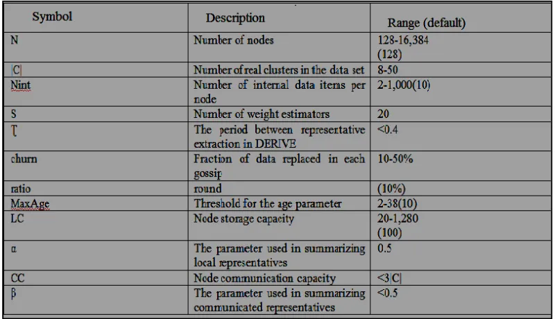
The second assignment strategy abates the average number of nodes that have data close to each other. Such a condition reduces the number of other nodes which have target data for the COLLECT task. When applying churn, in the first assignment strategy, data items are replaced with random unassigned data items. The second data assignment strategy allows concept drift when applying churn, by reserving some of the clusters and selecting new points from these clusters. Concept drift refers to change in statistical properties of the target data set which should be clustered. Nodes can adjust the r parameter during execution based on the incurred communication complexity. In the evaluations, for simplicity, the r parameter is selected such that the average number of data located within the r radius of each data item is equal to 5. Different parameters used in conducting the experiments, along with their value ranges and defaults, are presented in Table 1. The parameter values are selected such that special behaviours of the algorithm are revealed. LC and CC are measured as multiples of the required resource for one representative. The majority of the evaluations are performed with partition- based clustering. Partial evaluation on density based clustering is discussed at the end of the section.

(8)

ISSN(Online): 2320-9801

ISSN (Print) : 2320-9798

I

nternational

J

ournal of

I

nnovative

R

esearch in

C

omputer

and

C

ommunication

E

ngineering

V. SEARCHING METHODOLOGIES

There are two types of search algorithms: algorithms that don’t make any assumptions about the order of the list, and algorithms that assume the list is already in order. We’ll look at the former first, derive the number of comparisons required for this algorithm, and then look at an example of the latter. In the discussion that follows, we use the term search term to indicate the item for which we are searching. We assume the list to search is an array of integers, although these algorithms will work just as well on any other primitive data type (doubles, characters, etc.). We refer to the array elements as items and the array as a list.

A. Linear Search:

The simplest search algorithm is linear search. In linear search, we look at each item in the list in turn, quitting once we find an item that matches the search term or once we’ve reached the end of the list. Our “return value” is the index at which the search term was found, or some indicator that the search term was not found in the list.

A1. Algorithm for linear search

for (each item in list) {

compare search term to current item if match,

save index of matching item break

}

return index of matching item, or -1 if item not found

A2. Performance of linear search

When comparing search algorithms, we only look at the number of comparisons, since we don’t swap any Values while searching. Often, when comparing performance, we look at three cases:

 Best case: What is the fewest number of comparisons necessary to find an item?

 Worst case: What is the most number of comparisons necessary to find an item?

 Average case: On average, how many comparisons does it take to find an item in the list?

 For linear search, our cases look like this:

 Best case: The best case occurs when the search term is in the first slot in the array. The number of comparisons in this case is 1.

 Worst case: The worst case occurs when the search term is in the last slot in the array, or is not in the array. The number of comparisons in this case is equal to the size of the array. If our array has N items, then it takes N comparisons in the worst case.

 Average case: On average, the search term will be somewhere in the middle of the array. The number of comparisons in this case is approximately N/2.

In both the worst case and the average case, the number of comparisons is proportional to the number of items in the array, N. Thus, we say in these two cases that the number of comparisons is order N, or O (N) for short. For the best case, we say the number of comparisons is order 1, or O (1) for short.

B. Binary Search:

(9)

ISSN(Online): 2320-9801

ISSN (Print) : 2320-9798

I

nternational

J

ournal of

I

nnovative

R

esearch in

C

omputer

and

C

ommunication

E

ngineering

lower, we eliminate the upper half of the list and repeat our search starting at the point halfway between the first item and the middle item. If it’s higher, we eliminate the lower half of the list and repeat our search starting at the point halfway between the middle item and the last item.

B1. Algorithm for binary search

set first = 1, last = N, mid = N/2 while (item not found and first < last) {

compare search term to item at mid if match

save index break

else if search term is less than item at mid, set last = mid-1

else

set first = mid+1 set mid = (first+last) }

return index of matching item, or -1 if not found

B2. Performance of binary search

The best case for binary search still occurs when we find the search term on the first try. In this case, the search term would be in the middle of the list. As with linear search, the best case for binary search is O(1), since it takes exactly one comparison to find the search term in the list.

The worst case for binary search occurs when the search term is not in the list, or when the search term is one item away from the middle of the list, or when the search term is the first or last item in the list. How many comparisons does the worst case take? To determine this, let’s look at a few examples.

Suppose we have a list of four integers: {1, 4, 5, 6}. We want to find 2 in the list. According to the algorithm, we start at the second item in the list, which is 4.2 Our search term, 2, is less than 4, so we throw out the last three items in the list and concentrate our search on the first item on the list, 1. We compare 2 to 1, and find that 2 is greater than 1. At this point, there are no more items left to search, so we determine that 2 is not in the list. It took two comparisons to determine that 2 is not in the list. Now suppose we have a list of 8 integers: {1, 4, 5, 6, 9, 12, 14, 16}. We want to find 9 in the list. Again, we find the item at the midpoint of the list, which is 6. We compare 6 to 9, find that 9 is greater than 6, and thus concentrate our search on the upper half of the list: {9, 12, 14, 16}.

We find the new midpoint item, 12, and compare 12 to 9. 9 is less than 12, so we concentrate our search on the lower half of this list (9). Finally, we compare 9 to 9, find that they are equal, and thus have found our search term at index 4 in the list. It took three comparisons to find the search term. If we look at a list that has 16 items, or 32 items, we find that in the worst case it takes 4 and 5 comparisons, respectively, to either find the search term or determine that the search term is not in the list. In all of these examples, the number of comparisons is log2 N3. This is much less than the number of comparisons required in the worst case for linear search! In general, the worst case for binary search is order log N, or O(logN). The average case occurs when the search term is anywhere else in the list. The number of comparisons is roughly the same as for the worst case, so it also is O(logN).

In general, anytime an algorithm involves dividing a list in half, the number of operations is O(log N).

VI. SIMULATION RESULTS

(10)

ISSN(Online): 2320-9801

ISSN (Print) : 2320-9798

I

nternational

J

ournal of

I

nnovative

R

esearch in

C

omputer

and

C

ommunication

E

ngineering

A. Static Settings

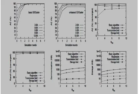
When network data is persistent, each node gradually learns the data through its representatives, and the clustering accuracy converges. The algorithm behavior in a static setting is shown in Fig.3, where the number of internal data items of each node, Nint , varies from 2 to 10. The trend of clustering accuracy convergence against simulation rounds, is shown for basic and enhanced GDCluster. Convergence is identified by three rounds of minor (less than 1 percent) change in results. The accuracy converges in to 100% and more than 95% in basic and enhanced GDCluster respectively. The enhanced GDCluster offers less converged accuracy values due to limited transmission of representatives and data, which reduces the quality of the constructed view of data in each node. As observed, in this setting, when nodes have few data (e.g., Nint = 2), detecting accurate clusters is harder, due to sparseness of clusters. The same figure compares the basic GDCluster with three improved versions, when Nint varies. Communication and storage overheads show average per round values until convergence for each node. The values are considerable for the basic GDCluster due to the storage and transmission of a large number of external data items and representatives. The first improved version involves regression to reduce the weight estimators. As expected, this improvement preserves the clustering accuracy, while reducing the resource consumption up to 80%. In the next improvement, the communication capacity is restricted. In this setting, the AC values decrease by approximately 2 percent, while the communication overhead experiences a major reduction. Further limitation of storage capacity in the last improvement, still keeps AC above 95%, but deallocates local resources.

(11)

ISSN(Online): 2320-9801

ISSN (Print) : 2320-9798

I

nternational

J

ournal of

I

nnovative

R

esearch in

C

omputer

and

C

ommunication

E

ngineering

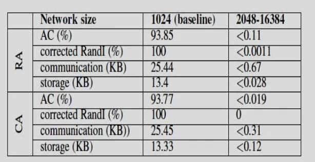
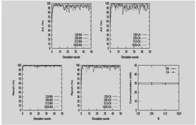
Fig. 4: It shows the behaviour of GDCluster when the network size varies from 1024 to 16384 nodes. The AC values have converged to more than 90%. This shows the efficiency and scalability of the algorithm. In the random data-assignment strategy, AC values are initially higher. This is due to each node initially having internal data items from different clusters, enabling it to identify more clusters. As the performance of the algorithm for different network sizes is very similar, we used the average values of different metrics for N = 1024 as a baseline in table 2, and showed the difference of values for other network sizes.Convergence in a static setting, when N varies (average values in table 2)

The RandI values converge to 100%. The communication and storage overheads of the algorithm remain constant due to restricting resource consumption. As observed, the differences of values for different network sizes are small, showing scalability of the algorithm. In the evaluation of the algorithm using real data sets, both central K means and GDCluster are evaluated against the actual labels of data, and the results are presented in Table 3. GDCluster is executed in a network of 1024 nodes, each having 10 data items. The AC and RandI values for GDCluster are very close to those of the central K-means. Because GDCluster executes K-means on the representatives instead of data, when compared to actual data labels, its accuracy may even surpass the central results for some data sets. The results show the efficiency of the algorithm in conforming to central clustering for real-world data.

(12)

ISSN(Online): 2320-9801

ISSN (Print) : 2320-9798

I

nternational

J

ournal of

I

nnovative

R

esearch in

C

omputer

and

C

ommunication

E

ngineering

Table 3: Average values of evaluation metrics for 50 runs of the algorithm with real data sets

B. Dynamic Settings

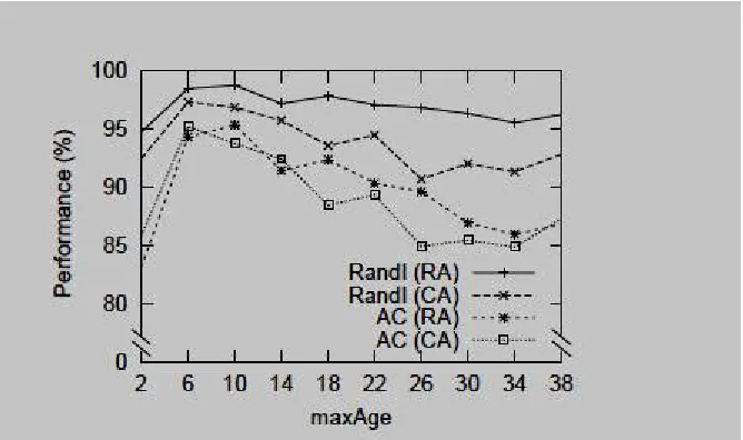
The MaxAge parameter puts an upper bound on the storage period of external data items, and representatives. Fig.5 shows the evaluation of the basic GDCluster algorithm when MaxAge varies. Very low values of MaxAge prohibit complete propagation of information in the network, and also cause early removal of data and representatives. Large values, on the other hand, maintain invalid information longer than required and degrade accuracy. The optimum behavior of the algorithm is observed when MaxAge is equal to 6.

Fig. 5. Effect of changing MaxAge

(13)

ISSN(Online): 2320-9801

ISSN (Print) : 2320-9798

I

nternational

J

ournal of

I

nnovative

R

esearch in

C

omputer

and

C

ommunication

E

ngineering

Fig. 6. Evaluation of GD Cluster in dynamic setting, when N varies.

With concept drift, nodes should move on to discover representatives in the new clusters. It also takes some time for the removed data to be discarded by the embedding representatives. Similar trends are observed for the RandI metric, where approximate average values of 98% and 96% are achieved for RA and CA strategies, respectively. The algorithm has acceptable performance in detecting clusters, even in dynamic settings. Finally the same figure shows that the communication overhead for different network sizes remains roughly the same. This is mainly due to removal of representatives in the dynamic setting which reduces the amount of transferred data between nodes.

C. Comparison with LSP2P

The LSP2P algorithm executes the K-means in an iterative manner, with each node synchronizing with its neighbors during each iteration. In a static setting, the algorithm is initiated at a single node p, which picks a set of random initial centroids along with a termination threshold g > 0 (which we explain shortly). P sends these to all its immediate neighbors, and begins iteration 1. When a node receives the initial centroids and threshold for the first time, it forwards them to its remaining neighbors and initiates iteration 1. In each iteration, every node p executes one round of K-means on its local data based on the centroids computed inthe previous iteration. It then prompts its immediate neighbors for their corresponding cluster centroids, and updates local centroids based on the received information. Once the computed centroids of two consecutive iterations, deviate less than g from each other, p enters the terminated state. In a dynamic setting, the change of data may reactivate the nodes. Regarding the above descriptions on LSP2P, it is observed that the initial centroids are identical in all nodes, which prohibits changing the number of produced clusters. Also, if K-means is to be executed with different initial centroids, a new instance ofLSP2P should be started. Moreover, the history of executing the K means algorithm is particularly important, and maintained in each node.

VII. CONCLUSION AND FUTURE WORK

(14)

ISSN(Online): 2320-9801

ISSN (Print) : 2320-9798

I

nternational

J

ournal of

I

nnovative

R

esearch in

C

omputer

and

C

ommunication

E

ngineering

Adaptability to dynamics of the data set was made possible by introducing an age factor which assisted in detecting data set changes updating the clustering model. Our experimental evaluation and comparison showed that the algorithm allows effective clustering with efficient transmission costs, while being scalable and efficient.

GD Cluster can be customized for other clustering types, such as hierarchical or grid-based clustering. To accomplish this, representatives can be organized into a hierarchy, or carry statistics of approximate grid cells. Further discussion of these algorithms is deferred to future work.

REFERENCES

1. K. M. Hammouda and M. S. Kamel, “Hierarchically distributed peer-to-peer document clustering and cluster summarization,” IEEE Trans. Knowl. Data Eng., vol. 21, no. 5, pp. 681–698, May 2009.

2. Y. Pei and O. Za€ıane, “A synthetic data generator for clustering and outlier analysis,” Dept. Comput. Sci., Univ. Alberta, Edmonton, AB, Canada, Tech. Rep. TR06-15, 2006.

3. M. Stonebraker, J. Frew, K. Gardels, and J. Meredith, “The sequoia 2000 storage benchmark,” in ACM SIGMOD Rec., vol. 22, no. 2, pp. 2–11, 1993.

4. N. Visalakshi and K. Thangavel, “Distributed data clustering: A comparative analysis,” in Foundations Computational Intelligence, vol. 206, A. Abraham, A.-E. Hassanien, A. de Leon, F. de Carvalho, and V. Snasel, Eds, Berlin, Germany: Springer-Verlag, 2009, pp. 371–397.

5. N. F. Samatova, G. Ostrouchov, A. Geist, and A. V. Melechko, “RACHET: An efficient cover-based merging of clustering hierarchies from distributed datasets,” Distrib. Parallel Databases, vol. 11, pp. 157–180, Mar. 2002.

6. M. Eisenhardt, W. Muller, and A. Henrich, “Classifying documents by distributed P2P clustering,” in Proc. Informatik, Sep. 2003, pp. 286 291. 7. R. Wolff, K. Bhaduri, and H. Kargupta, “A generic local algorithm for mining data streams in large distributed systems,” IEEE Trans. Knowl.

Data Eng., vol. 21, no. 4, pp. 465–478, Apr. 2009.

8. K. Tasoulis and M. N. Vrahatis, “Unsupervised distributed clustering,” in Proc. IASTED Int. Conf. Parallel Distrib. Comput. Netw., 2004, pp. 347–351.

9. H.-P. Kriegel, P. Kunath, M. Pfeifle, and M. Renz, “Approximated clustering of distributed high-dimensional data,” in Proc. 9th Pacific-Asia Conf. Adv. Knowl. Discovery Data Min., 2005, pp. 432–441.

10. L. M. Aouad, N.-A. Le-Khac, and T. M. Kechadi, “Lightweight clustering technique for distributed data mining applications,” in Proc. 7th Int. Conf. Data Mining, 2007, pp. 120–134.

11. S. Merugu and J. Ghosh, “A privacy-sensitive approach to distributed clustering,” Pattern Recognit. Lett., vol. 26, no. 4, pp. 399–410, 2005. 12. A. Elgohary, “Scalable embeddings for kernel clustering on mapreduce,” M.Sc. Thesis, Electrical and Computer Engineering, Univ. Waterloo,

Waterloo, ON, Canada, 2014.

13. Eyal, I. Keidar, and R. Rom, “Distributed data clustering in sensor networks,” Distrib. Comput., vol. 24, no. 5, pp. 207–222, 2011.

14. G. Di Fatta, F. Blasa, S. Cafiero, and G. Fortino, “Fault tolerant decentralised k-means clustering for asynchronous large-scale networks,” J. Parallel Distrib. Comput., vol. 73, no. 3, pp. 317–329, 2013.

15. P. Shen and C. Li, “Distributed information theoretic clustering,” IEEE Trans. Signal Process., vol. 62, no. 13, pp. 3442–3453, Jul. 1, 2014.

BIOGRAPHY

Vikram A. received B.E degree in Electrical and Electronics Engineering, M.E. degree in Computer Science and Engineering from V.S.B Engineering College in 2006 and from Pavender Bharathidasan College of Engineering and Technology in 2008 and Master of Business Administration in Project Management from Alagappa University in 2012 respectively. Currently he is working as an Assistant Professor in Saranathan College of Engineering, Tiruchirappalli, Tamil Nadu

(15)

ISSN(Online): 2320-9801

ISSN (Print) : 2320-9798

I

nternational

J

ournal of

I

nnovative

R

esearch in

C

omputer

and

C

ommunication

E

ngineering

S.Vinothini, Student, IV year Bachelor of Engineering in Computer Science and Engineering, Department of Computer Science and Engineering, Saranathan College of Engineering, Tiruchirappalli, Tamil Nadu. She is a bright, meritorious and meticulous student with keen interest in research arena.

A.Shivapriya, Student, IV year Bachelor of Engineering in Computer Science and Engineering, Department of Computer Science and Engineering, Saranathan College of Engineering, Tiruchirappalli, Tamil Nadu. She is a bright, meritorious and meticulous student with keen interest in research arena.