Evaluating the Effects of FDI on Growth in the Context of One and Two-Sector Endogenous Growth Models.

(1)

ABSTRACT

KONDYAN, SERGEY SERGO. Evaluating the Effects of FDI on Growth in the Context of One and Two-Sector Endogenous Growth Models. (Under the direction of John J. Seater.)

In my dessertation research I develop a theoretical framework that focuses on the pure

effects of FDI on growth in the absence of technology transfers or other channels through

which the spillover effects of FDI can operate. By isolating the effects of FDI on growth

from the presence of the alternative channels of transmission I address the issue of what

FDI by itself does for growth through its primary function of capital accumulation. I study

growth effects of FDI in the context of an endogenous growth model with one and two

sectors of production where growth is generated by perpetual accumulation of capital. As

the results suggest, the growth effects of FDI depend on technological differences across

countries. If countries are technologically the same then FDI does not generate any growth

effects for either home or host country. If, however, countries are technologically different

with the home country being technologically advanced in the FDI conducting sector then

the home country will not experience any growth effects, whereas the host country will

face negative growth effects due to reduction of the marginal product of capital resulting

from the process of capital accumulation through FDI. The transitional behavior of both

countries in the presence of FDI is different from the dynamics of closed economy, one and

two-sector models with endogenous growth. The difference comes from the fact that the

behavior of the variables in the host country depends on the behavior of the variables in

the home country through the FDI channel which suggests that the transitional behavior

of host and home countries should be analyzed together, through the multidimensional

(2)

dimensionality of this dynamic system does not lead to analytical solutions, and I use

(3)

(4)

Evaluating the Effects of FDI on Growth in the Context of One and Two-Sector Endogenous Growth Models

by

Sergey Sergo Kondyan

A dissertation submitted to the Graduate Faculty of North Carolina State University

in partial fulfillment of the requirements for the Degree of

Doctor of Philosophy

Economics

Raleigh, North Carolina

2012

APPROVED BY:

Douglas Pearce Asli Leblebicioglu

Ivan Kandilov John J. Seater

(5)

DEDICATION

To my wife Karine

and

(6)

BIOGRAPHY

Sergey Kondyan was born in Ninotsminda, Georgia. He graduated from Yerevan

Poly-technic Institute in 1991 with Electric Engineer Diploma. He continued his education in

the State Engineering University of Armenia in the area of Control System Engineering

and received his Master of Engineering diploma in 1994. Continuing his education in

the area of Control System Engineering in the same university in 1996 he completed the

program and received Engineer-Researcher diploma.

While he was in the Graduate School Sergey Kondyan combined his education with

part time administrative job at Yerevan University of Management and Information

Technology (YUMIT), and starting from September 1996 he moved to the full time

appointment in the position of the Deputy Dean of the Preliminary Department.

Sergey Kondyan started his teaching career at YUMIT in 1996, where he taught

Principles of Economics course and supervised several diploma works, first in the

De-partment of Economics and Finance, and later in the DeDe-partment of Applied Economics

and System Analysis at YUMIT.

In 2006 Sergey Kondyan received full Graduate Teaching Assistantship to pursue

master studies in economics and continued his education in the Department of Economics

at East Carolina University. He completed the program within one year and received his

Master of Science in Economics degree in December 2006.

In 2007 he received full graduate teaching assistantship to pursue PhD degree in

Economics at NCSU. During the years of education at NCSU Sergey Kondyan developed

fields in Economic Growth and Industrial Organization. At NCSU he also worked as

an instructor for Principles of Macroeconomics, and Introduction to Agricultural and

(7)

In the fall 2011 Sergey Kondyan worked as an Adjunct Assistant Professor, in the

Department of Economics at Elon University.

(8)

ACKNOWLEDGEMENTS

I would like to thank my advisor, Dr. John Seater, for all his help, encouragement,

patience, and support through my work on this dissertation project. His insights and

comments were invaluable and this dissertation would not be completed without his

advice.

I also would like to thank all my committee members Dr. Douglas Pearce, Dr. Asli

Leblebicioglu and Dr. Ivan Kandilov for their useful comments and continuous support

throughout this dissertation work.

I thank all Triangle Dynamic Macro (TDM) Workshop participants for their valuable

comments and suggestions. Particularly, I would like to thank Dr. Pietro Peretto and Dr.

Michelle Connolly for their insights and suggestions.

I also would like to thank all the faculty and staff in the Department of Economics

at North Carolina State University for their important contribution to my professional

development.

Finally, I would like to thank my wife Karine and my daughters Anahit and Christine

(9)

LIST OF FIGURES

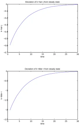
Figure 3.1 Deviation of ˆkjt, and ˜kit from steady-statel . . . 88

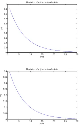
Figure 3.2 Deviation of cit, and cjt from steady-statel . . . 89

Figure 3.3 The transition path of ˆkjt, and ˜kit . . . 90

Figure 3.4 The transition path of cit, and cjt . . . 91

Figure 3.5 The transition path of r_Kjtˆ , and ˙ Cit Cit . . . 92

(11)

Chapter 1 A One-Sector Model with Foreign

Direct Investment

1.1 Introduction

There has been a substantial increase in the flow of foreign direct investment (FDI)

in recent years. For the United States alone direct investment abroad increased from

$209,392 million in 1999 to $328,905 million in 2010, which translates to a 57% increase

in US capital outflows over the indicated period.1

Despite quite significant increases in FDI flows, there is little resarch on the different

aspects of FDI, in particular the effects of FDI on growth. The objective of the current

work is to study growth effects of FDI through the process of capital accumulation, which

is a primary benefit that FDI brings to a host country. To the best of my knowledge this

work is the first study of the growth effects of FDI through its primary function of capital

accumulation.

(12)

In the existing literature the theoretical and policy arguments on the positive effects

of FDI on growth are considered mainly through the positive spillover mechanism of

FDI in the form of technological transfers, training of the labor force, and networks etc.

On empirical grounds, however, there is no strong evidence that FDI promotes growth

through spillover mechanisms.

Lipsey (2002) addresses different aspects of the potential effects of FDI in his review

of the empirical literature on the subject. Among other things, he considers the

empir-ical evidence on the productivity spillovers from FDI and argues that the evidence of

productivity spillovers is mixed.

Micro empirical evidence based on the studies using firm-level data for different

coun-tries supports Lipsey’s claim. Blomstrom and Wolff (1994), for example, found that

in-creased foreign presence contributed to an increase in productivity of Mexican firms

relative to US productivity levels between 1965 and 1982. On the contrary, Aitken and

Harrison (1999), using plant level data on Venezuela, argue that FDI has a negative effect

on productivity of domestically-owned plants, even though it may increase productivity

of the plants receiving FDI. Harrison and McMillan (2003), using firm data on the Ivory

Coast, provide evidence that not only are domestic firms more credit constrained

com-pared to foreign firms but also the excessive borrowing by foreign firms in the domestic

market “exacerbates domestic firm credit constraints”, making the argument on positive

productivity spillovers of FDI quite weak.

In terms of the macroeconomic literature, the studies do not find systematic evidence

that FDI in itself raises growth. Given the relevance of the current work to the

macroe-conomic literature I would like to discuss macroemacroe-conomic results on the effects of FDI in

more details.

(13)

channel of technology transmission and therefore contribute to faster growth only in the

host countries that have some minimum threshold stock of human capital. Their

empir-ical approach is built on the theoretempir-ical framework of endogenous growth models with

variety expansion, discussed among others by Barro-and Sala-i-Martin (2004). The stock

of physical capital in the economy is an aggregate of the varieties of the capital goods.

The endogenous growth in the model is therefore generated by the accumulation of the

aggregate capital stock through the process of expansion of the varieties of capital goods.

The varieties can be expanded by both domestic and foreign firms. New varieties require

adaptation of technology and thus incur fixed setup costs, which negatively depend on

the ratio of foreign firms to the total number of firms in the economy. The latter

as-sumption captures the notion that foreign firms bring advanced technology to the host

country. Borensztein, De Gregorio and Lee show that under their model specification FDI

increases growth through reducing the costs of introducing new varieties and increasing

the rate of introduction of new varieties. What is important for their empirical analysis is

the positive association between the growth rate of the economy and the level of human

capital that the economy is endowed with. The authors argue that the positive

relation-ship between human capital and growth suggests that the effect of FDI on growth can

be stronger in countries with higher endowments of human capital; the argument they

tested empirically. Even though this conclusion directly follows from the specification of

the production technology, nevertheless empirical analysis using panel data on FDI flows

from industrialized to 69 developing countries, covering the periods from 1970 to 1979

and 1980 to 1989, provides robust evidence that the effect of FDI on growth depends on

the level of human capital in the host country. This evidence combined with the other

results of empirical analysis leads to a more general conclusion that the positive growth

(14)

advanced technologies” in the host countries.

Alfaro, Chanda, Kalemi-Ozcan and Sayek (2004, 2009) provide more evidence on the

“absorptive capability” argument by exploring the role financial markets play in fostering

the effects of FDI on growth. Their empirical study (2004) suggets that the growth effects

of FDI are possible only in the presence of well-developed financial markets that lead to

easier adaptation of advanced technologies brought in by FDI.

In their later study (2009) Alfaro, Chanda, Kalemi-Ozcan and Sayek develop a

the-oretical formalization of their empirical framework on the role of financial markets in

promoting the positive effects of FDI on growth through backward linkages that

gener-ate positive spillovers for the whole economy.2 _{As they argue, the failure of researchers}

to find empirical evidence of positive technological spillovers of FDI can be linked to the

idea that foreign firms want to use the ownership advantage that they have to

“outper-form local firms”. Their approach, therefore, is to model benefits from FDI as “occurring

via linkages and not through technology spillovers”.

Similar to Borensztein, De Gregorio and Lee (1998), the theoretical structure

devel-oped by Alfaro, Chanda, Kalemi-Ozcan and Sayek is essentially an open-economy version

of variety expansion model with endogenous growth.3 _{They use a small open economy}

setup characterized by two industry streams. “The downstream industry” produces the

final consumption good by using two intermediate inputs that differ from each other

based on their country of ownership. The production of these intermediate inputs in its

turn constitutes ”the upstream industry” and requires a combination of skilled and

un-skilled labor and an array of differentiated inputs. The evolution of the varieties of those

intermediate inputs generates the mechanism of endogenous growth in the model. The

2_{Backward linkages are defined as: “contacts between domestic suppliers of intermediate inputs and}

their multinational clients in downstream sectors”.

(15)

link between foreign firms and the level of development of financial markets in the host

country arises from the need of foreign firms to finance their upfront investment into

developing the new varieties of the capital inputs. The costs of borrowing resources from

the domestic financial markets reflect the degree of the development of financial markets

in the host country. The results of the calibration exercise show that an increase in the

share of FDI contributes more to growth in financially developed countries, supporting

the claims that there is no evidence on the exogenous effects of FDI on growth and that

the ability of FDI to affect growth depends on the “absorptive capability” of the host

country, which in this particular study is captured by the level of financial development

of the host country.

Earlier work by Carkovic and Levine (2002) also supports the conclusion that there is

no robust evidence on the positive effects of FDI on growth. As they argue, “there is not

reliable cross-country empirical evidence supporting the claim that FDI per se accelerates

growth”.

Even though on empirical grounds the evidence for the exogenous effect of FDI on

growth is weak if not absent at all, the theoretical framework explaining this phenomenon

and addressing the issue of what FDI itself does to growth seems to be missing. My

dissertation work fills in this gap in the literature by developing a theoretical framework

focusing on the pure effects of FDI on growth through its primary function of capital

accumulation. Researchers in fact do emphasize the importance of FDI as a source of

capital accumulation but in the meantime they acknowledge the lack of a literature

focusing primarily on the capital accumulation role of FDI.

In the abovementioned survey of the literature on FDI, Lipsey (2002) argues that in

addressing the issues related to efficiency of foreign operations in the host country and

(16)

researchers use measures of efficiency ranging from “value added per unit of labor input,

the simplest, to value added per unit of labor and capital input and value of output per

unit of labor, capital and intermediate product input”. As he continues “most authors

seem to prefer the efficiency measures including capital input. The result is to ignore any

host country benefit from the accumulation of physical capital, or from any advance in

technology that consists of the adoption of more capital intensive methods of production

or larger scale production”.

In the aforementioned work by Borensztein, De Gregorio and Lee (1998), the

au-thors do test the effect of FDI on growth through the process of augmenting capital

accumulation in the host country. In particular, they consider the effect of FDI on total

investment, arguing that if the coefficient on FDI equals 1 then it suggests that FDI does

not increase total investment in a host country, while a coefficient more than one implies

that FDI actually leads to a “crowding-in” effect. As their results suggest, the data show

that FDI stimulates domestic investment and that there is a complementarity between

foreign and domestic investment, however this result is not robust across different model

specifications used by the authors.

The lack of work focusing on the effects of FDI on growth through its primary

func-tion of capital accumulafunc-tion can be explained, at least to some extent, by the lack of

evidence on the growth effects of capital accumulation. Jones (1995) argues that there is

no empirical evidence on the positive long-run growth effects of investment. Easterly and

Levine (2001) in their review of the empirical literature on growth conclude that there is

no evidence that factor accumulation contributes to faster growth of output per worker.

In their recent study, Bond, Leblebicioglu and Schiantarelli (2010) reassess the

em-pirical relationship between investment in physical capital and long-run growth. In their

(17)

evidence on the positive relationship between investment, measured as a share of GDP

and long-run growth. Their methodology is based on controlling for country specific fixed

effects and focusing on time-varying control variables. The advantage of this methodology

is that it controls for country-specific factors such as political and institutional

infras-tructure that could potentially influence the relationship between investment and growth.

As they conclude, “our results suggest that investment is at least an informative proxy,

and are consistent with investment being an important channel through which deeper

causes influence growth outcomes. Growth theories that predict a positive relationship

between investment and long-run growth rates should not be dismissed as being grossly

inconsistent with the empirical evidence”.

Lack of a literature on FDI, its increasing role, and disagreements between theoretical

and empirical literature serve as important motivational factors for current work. In this

work I develop a theoretical framework that focuses on the pure effects of FDI on growth

in the absence of technology transfers or any other channel through which spillover effects

can operate. By isolating the effects of FDI on growth from the presence of alternative

channels of transmission I address the issue of what FDI by itself does for growth through

its primary function of capital accumulation.

My theoretical framework is based on one and two sector endogenous growth model

structures discussed in Barro and Sala-i-Martin (2004). I have developed an open-economy

extension of both one and two sector endogenous growth models to study the growth

effects of FDI. The choice of model structures is motivated by the following

character-istics. Both one and two sector endogenous growth models have tractable structures.

Endogenous growth is generated by perpetual accumulation of capital, which is exactly

the structure that I need to study the growth effects of FDI from capital accumulation.

(18)

one sector model both types of capital are assumed to be perfect substitutes produced

within the single sector of an economy. This simplified structure serves as a benchmark

for study of FDI in the context of endogenous growth with accumulation of capital, which

is discussed in the first chapter of my dissertation.

In the second chapter I utilize the simplified two sector structure of the

Uzawa-Lucas model (Uzawa (1965), Uzawa-Lucas (1988)). The model separates the production of both

types of capital into two different sectors of the economy. This structure allows one to

distinguish between domestic and foreign investment in physical capital and domestic

production of human capital. As emphasized in the literature, sectoral decomposition of

the production process is an important aspect in the study of the growth effects of FDI.

In particular, Lejour and Rojas-Romagosa (2006) argue that most policy prescriptions

aimed to increase flows of FDI are sector specific, for example the Services Directive by

the European Commission, and the GATS proposals aimed to reduce trade barriers in

services. Alfaro (2003) shows that the growth effects of FDI differ substantially across

different sectors of the economy, being negative in the primary sector, positive in the

manufacturing sector and ambiguous in the services sector.

In the third chapter I extend my analysis to incorporate FDI into the more general

structure of a two sector model. The richer framework of this model allows me to introduce

FDI not only in physical capital, but also in the other type of capital, which can be

interpreted as human capital or any other type of capital that augments labor but is not

embodied in labor.4

Another important characteristic of this class of endogenous growth models is that

the closed economy versions of one and two-sector endogenous growth models generate

very interesting patterns of transitional dynamics. Adopting the structure of these models

(19)

allows one to focus not only on the long-run but also on the transitional effects of FDI

on growth.

Across all three models I assume that the production process is described by a

per-fectly competitive structure to avoid the complications arising from potential strategic

games played by countries in an attempt to manipulate rates of return on capital. There

is also no borrowing or lending via credit markets either within or across countries.

The results of the analysis suggest that technological differences across countries play

an important role in determining the growth effects of FDI from capital accumulation. If

countries have the same level of technology then there are no long-run growth effects of

FDI. This result is consistent with the aforementioned empirical evidence on the absence

of exogenous effects of FDI on growth.

If, however, countries are technologically different then the host country will

experi-ence negative growth effects from FDI.

The transitional behavior of both countries in the presence of FDI is different from

the dynamics of the closed economy one or two sector models with endogenous growth.

The difference comes from the fact that the behavior of the variables in the host country

depends on the behavior of the variables in the home country through the FDI channel.

This suggests that the transitional behavior of host and home countries should be

ana-lyzed together, through the multidimensional system of differential equations describing

the transitional path of both countries. Even though the dimensionality of the dynamic

system does not lead to an analytical solution, I use model calibration techniques to

(20)

1.2 The Setup of the Model

Before I introduce FDI into the framework of a one sector endogenous growth model

I will briefly summarize the setup of the model under autarky, discussed in Barro and

Sala-i-Martin (2004, chapter 5).

1.2.1 The Model Under Autarky

In autarky the total output produced in the economy (Y) is used for consumption and

domestic investment in two types of capital, K and H. Under the assumption of a

Cobb-Douglas production process the resource constraint for an economy is written as:

Y =AKαH1−α =C+IK+IH (1.1)

where IK and IH are gross investments in the K and H type of capital respectively.

Assuming that both types of capital depreciate at the same rate δ, gross investment

is:

IK = ˙K+δK (1.2)

and

IH = ˙H+δH (1.3)

Household preferences are described by the following CRRA utility function:

U =

Z ∞

0

U(Ct)e−ρtdt (1.4)

where

U(Ct) =

(21)

The optimization problem faced by a country can be written as the maximization

of (1.4) subject to the resource constraint (1.1) and accumulation conditions (1.2) and

(1.3), which leads to the following present value Hamiltonian.

V = C

1−θ t −1

1−θ e

−ρt

+µ1(IK −δK) +µ2(IH −δH) +λ(AKαH1−α−C−IK−IH)

The growth rate of consumption is derived from the necessary conditions of this

optimization problem :

˙

C

C =

1

θ Aα

K H

α−1

−δ−ρ

!

The no arbitrage condition requires equalization of the marginal products of K and

H capital, which leads to the solution of K to H ratio as follows:

Aα

K H

α−1

=A(1−α)

K H

α

K

H =

α

1−α (1.5)

Constancy of K_H implies equalization of the growth rates of K and H. It is also shown

that growth rates of C and Y are constant and equal to the growth rates of K and H.

Substituting the expresion for K_H into the solution for the growth rate of consumption

will result in the solution for the common growth rate of this autarkic economy given by:

γAu=

1

θ Aα

α₍₁₋_α₎1−α₋_δ₋_ρ

(1.6)

The important argument in the discussion of the transitional dynamics of a one-sector

endogenous growth model is the assumption of irreversible investment, which

(22)

country cannot dissinvest in either type of capital. Therefore, each time the country

devi-ates from the value of the K to H ratio given in (1.5) one of the constraints of irreversible

investment becomes binding and country sets that investment equal to 0.

The inequality constraints create the main foundation in the study of transitional

dynamics of the autarkic version of the one sector model discussed above. In particular,

as it follows from the assumption of irreversible investment, only one type of capital will

be accumulated along the transition reducing the expression in (1.1) to either

Y =AKαH1−α=C+IK

or

Y =AKαH1−α =C+IH

depending on the deviation of the ratio of K to H capital from its steady state value.5

1.2.2 The Open-Economy Setup of the Model

In this section I incorporate FDI into a macro framework using the structure of the

one sector endogenous growth model with two types of capital discussed above. Here I

assume that the two types of capital are physical and human capital and that the country

conducts foreign investment only in physical capital.

To introduce FDI I need to distinguish between capital ownership and the capital

used in the production process.

Note that in the production process a country can only use the capital located within

its borders. Thus I can distinguish between total K type capital ownership and K capital

5_{For the detailed discussion of the transitional dynamics of a closed economy, one-sector endogenous}

(23)

used in the production process as follows:

ˆ

Kit = ¯Kit−K˜it,Kˆjt = ¯Kjt+ ˜Kit. (1.7)

where ˆKit denotes K capital produced in home country, ¯Kit denotes the total K capital

ownership for country i, and ˜Kit is capital created as an outcome of FDI. Similarly, ˆKjt

is the total K type capital used in the production in country j, and ¯Kjt is the total K

type capital ownership in country j. Here I explicitly assume that index i denotes the

home country that conducts FDI and index j denotes the host country - recipient of FDI.

The intuition behind the above expressions is as follows: if a country chooses to invest

abroad, then its total capital ownership will consist of capital produced domestically

and capital produced in the foreign country as an outcome of foreign direct investment.

On the other hand if country receives FDI then its total capital ownership will consist

of capital accumulated through the process of domestic investment only, while capital

used in production will be equal to the capital stock created through both domestic and

foreign investment.

The usual accumulation conditions for ˆKit, ˜Kit and ˆKjt are:

˙ˆ

Kit =I_Kitˆ −δKˆit,K˙˜it =I_Kit˜ −δK˜it,K˙ˆjt =I_Kjtˆ −δKˆjt. (1.8)

From (1.7) it follows that the accumulation of total capital stock owned by country i

will be given as:

˙ˆ

Kit= ˙¯Kit−K˙˜it

Using this equality I can now derive the resource constraint for country i in the

(24)

investments in the K and H type capital and foreign investment in the K type capital.

In addition, country i receives returns on the capital that it owns in the host country,

which will be given by the term rjtK˜it.

The overall resource constraint for country i can therefore be written as:

Yit+rjtK˜it=Cit+I_Kitˆ +IHit +I_Kit˜ (1.9)

where rˆ_kjt =αjAjKˆ αj−1

jt H

1−αj

jt is the rental rate on physical capital in the host country.

The optimization problem that country i faces can be summarized as maximization

of (1.4) subject to the above resource constraint.

So, the present value Hamiltonian (PVH) and the necessary conditions for country i

will be given by:

Jit =

C_it1−θ−1

1−θ e

−ρt₊_ψ

it(I_Kit˜ −δK˜it) +µit(IHit −δHit)

+φit h

AiKˆitαiH

1−αi

it −Cit−δKˆit−IHit−I_Kit˜ +rˆ_kjtK˜it i

∂Jit

∂Cit

=C_it−θe−ρt−φit= 0 (1.10)

∂Jit

∂I_Kit˜

=ψit−φit = 0 (1.11)

∂Jit

∂IHit

=µit−φit = 0 (1.12)

˙

φit=−

∂Jit

∂Kˆit

=−φit h

AiαiKˆαi

−1

it H

1−αi it −δ

i

(1.13)

˙

ψit =−

∂Jit

∂K˜it

(25)

˙

µit=−

∂Jit

∂Hit

=−µit[−δ]−φit h

Ai(1−αi) ˆKitαiH

−αi it

i

(1.15)

Initial and transversality conditions are omitted for simplicity.

To write the optimization problem for the host country it will be useful to simplify

the resource constraint as follows. I will start with the following expression:

Yjt =Cjt+I_Kjtˆ +IHjt −I_Kit˜ +rjtK˜it (1.16)

The above expression incorporates the flow of FDI from the home country given by

I_Kit˜ , which I can rewrite using the equation (1.8) as follows:

Yjt =Cjt+K˙ˆj−K˙˜i+δKˆj −δK˜i+IHjt +rjtK˜it (1.17)

Using the definitions in (1.7) I can simplify the above expression as:

Yjt =Cjt+ ˙¯Kj +δK¯j+IHjt +rjtK˜it (1.18)

Finally, I can express the resource constraint in the host country as an accumulation

condition for the domestically produced capital ¯Kj.

˙¯

Kj =Yjt−Cjt−IHjt −rjtK˜it−δK¯j (1.19)

This final expression is used to write the present value Hamiltonian and the necessary

conditions for country j:

Jjt =

C_jt1−θ−1

1−θ e

−ρt₊_µ

(26)

+φjt h

AjKˆ αj jt H

1−αj

jt −Cjt −δK¯jt−IHjt −rˆ_kjtK˜it i

∂Jjt

∂Cjt

=C_jt−θe−ρt−φjt = 0 (1.20)

∂Jjt

∂IHjt

=µjt−φjt = 0 (1.21)

˙

φjt =−

∂Jjt

∂K¯jt

=−φjt h

αjAjKˆ αj−1

jt H

1−αj jt −δ

i

(1.22)

˙

µjt =−

∂Jjt

∂Hjt

=−µjt[−δ]−φjtAj(1−αj) ˆK αj jt H

−αj

jt (1.23)

Again, the initial and transversality conditions are omitted for simplicity.

1.3 The Balanced Growth Path Solution

From the equations (1.11), (1.12), and (1.21) it follows that there is a bang-bang control

problem in investment. The necessary conditions for the choices of domestic and foreign

investment do not depend on the investment itself.

Each of the corresponding costate variables represents the marginal value of an

in-vestment:ψi is a marginal value of foreign investment for country i,φis a marginal value

of the domestic investment in K type capital andµis a marginal value of the investment

into H type capital for either country. The ratios of these costate variables represent

internal relative values of one type of investment in terms of the other. The ratio of ψi_φi is

the relative price of foreign investment in terms of the domestic investment for country

i and the ratio of µ_φ is the internal price of domestic investment in H capital in terms of

the domestic investment in K capital in either country.

The balanced growth path (BGP) solution requires that all variables are either

(27)

the BGP then constraints of irreversible investment can become binding for some types

of investment, violating the requirement of balanced growth. Therefore, for all types of

investment to be positive their marginal values must be equalized, otherwise a country

will have an incentive to invest in one type of capital and set investment in another type

of capital equal to 0 to satisfy inequality restrictions given byI_Kitˆ ≥0,I_Kit˜ ≥0,IHit ≥0,

I_Kjt¯ ≥ 0, and IHjt ≥ 0. Equalization of the marginal values of all investments implies

constancy of the internal prices as well; however marginal values are not necessarily equal

along the transition. They change according to their laws of motion given by equations

(1.13), (1.14), (1.15), (1.22) and (1.23).

I follow the approach discussed in Barro and Sala-i-Martin (2004) and first proceed

with the BGP solution where all investments are positive.

If all types of investment are positive for country i then the necessary conditions for

the optimal control problem will be given by (1.10) - (1.15). I can start with the solution

for the growth rates of the costate variables.

From (1.12) and (1.15) I can write:

˙

µi

=δ−Ai(1−αi) ˆKiαiH

−αi

i (1.24)

Then by combining (1.11) and (1.14) I will get:

˙

ψi

=δ−rj (1.25)

Finally from (1.13) it follows:

˙

φi

=δ−AiαiKˆiαi−1H

1−αi

(28)

Using the necessary condition for the choice of consumption and combining it with

the above solution for the growth rate of costate variable φ I obtain the growth rate of

consumption in country i as a function of the ratio of K_Hˆ as follows:

˙

Ci

= 1

θ

AiαiKˆαi

−1

i H

1−αi

i −δ−ρ

(1.27)

I have already argued that if all investments are strictly positive, then the no-arbitrage

condition requires equalization of the marginal values of each investment, which also

implies equalization of the growth rates of all costate variables. By setting them equal I

can solve for the value of the ratio of ˆK to H as follows:

AiαiKˆiαi−1H

1−αi

i −δ =Ai(1−αi) ˆKiαiH

−αi

i −δ =rj −δ (1.28)

AiαiKˆαi

−1

i H

1−αi

i =Ai(1−αi) ˆKiαiH

−αi i

ˆ

Ki

Hi !∗

= αi

1−αi

(1.29)

It follows from the above solution that this ratio is constant on the BGP and is

similar to the solution of K to H ratio under autarky (see equation (1.5)). The important

difference between these two ratios is the notion of K type capital represented in each

of them. In the presence of FDI ˆK measures the total capital stock produced within

the country, which is not equal to the capital stock owned by country i. Under autarky

the two concepts of K type capital stock (capital owned and capital used in production)

coincide.

Having solved for the ratio, I can substitute it into the solution for the growth rate

(29)

˙ Ci Ci !∗ = 1 θ

ααi_i Ai(1−αi)1

−αi ₋

δ−ρ

(1.30)

where r∗_i =ααi_i Ai(1−αi)

1−αi

is the steady state rate of return on capital in country i.

Following similar steps for country j I can solve for the growth rate of consumption

in country j.

First, using (1.21) and (1.23) I can derive the growth rate of the costate variable µ:

˙

µj

=δ−Aj(1−αj) ˆK αj j H

−αj

j (1.31)

Then from (1.22) I can derive the growth rate of costate variable φ equal to:

˙

φj

=δ−αjAjKˆ αj−1

j H

1−αj

j (1.32)

Combining the necessary condition for choice of consumption (1.20) with the above

solution for the growth rate of φI can write the solution for the growth rate of

consump-tion as: ˙ Cj Cj = 1 θ h

αjAjKˆ αj−1

j H

1−αj

j −δ−ρ i

(1.33)

Using (1.31) and (1.32) I can solve for the ratio of K to H type capital in country j

as follows:

AjαjKˆ αj−1

j H

1−αj

j =Aj(1−αj) ˆK αj j H −αj j ˆ Kj Hj !∗

= αj

1−αj

(1.34)

Again, the ratio of K to H capital is constant and is similar to the solution under

(30)

differ-ence in the ratios is related to the concept of K capital. Since country j is a recipient of

FDI, ˆK represents not only capital produced by country j but also the capital stock in

country j accumulated through FDI.

Substituting (1.34) into (1.33) we get the growth rate of consumption in country j.

˙

Cj

Cj !∗

= 1

θ

ααj_j Aj(1−αj)

1−αj

−δ−ρ (1.35)

Similarlyr_j∗ =ααj_j Aj(1−αj)

1−αj

is the steady state rate of return on capital in country

j.

Comparison of the growth rates of consumption for either country in the presence of

FDI given by (1.30) and (1.35) with the growth rate of consumption under autarky in

(1.6) reveals that there are no growth effects of FDI. There are, however, level effects of

FDI for both home and host countries. Country i has increased its total K type capital

stock, by accumulating capital through both domestic and foreign investment. I have

already argued that the ratio Ki_Hiˆ for country i is the same as under autarky, but it only

reflects K type capital accumulated domestically.

For the host country the ratio Kj_Hjˆ also reflects K type capital produced within country,

but in the presence of FDI it incorporates K type capital owned by the home country,

which suggests that host country owns a smaller stock of capital in the presence of FDI

compared to the scenario under autarky.

To finalize the BGP solution I show (see Appendix A) that on the BGP growth rates

of the variables are equalized across countries, such that there exists a common growth

rate defined as γ∗.

Note that equalization of the growth rates across countries does not necessarily imply

(31)

tech-nological differences across countries are captured by both total factor productivity and

factor share parameters. From the equalization of the growth rates across countries it

follows that r∗_i =r∗_j or alternatively:

Aiααii (1−αi)1−αi =Ajα αj

j (1−αj)1−αj

which implies that not only technologically identical countries can grow at the same rate

on the BGP in the presence of FDI. Countries can grow at the same rate but still differ

in terms of TFP and factor share parameters.

The BGP solution of the model in the presence of FDI generates at least two

interest-ing results: it follows that FDI does not generate any growth effects for both home and

host countries, and that equalization of the growth rates across countries in the presence

of FDI can be achived even for technologically different countries.

The above expression on the relationship between technological parameters on the

BGP in the presence of FDI across countries raises an interesting question on the

be-havior of the model if the technological parameters of both countries do not satisfy that

requirement with equality such that one of the countries has a higher long-run rate of

return on capital.

Note that as it follows from Aiααii (1−αi)1−αi and Ajα αj

j (1−αj)1−αj the steady state

rental rate of capital is determined by both TFP and the factor share parameters of each

country. If one of the countries has a higher long-run rate of return on capital then the

investment in that country is always more productive compared to another country. This,

in turn, implies that in the absence of barriers to openness, a country with a lower rate

of return on capital has an incentive to continuously shift its resources to the country

(32)

in the usual sense. A continuous shift of resources from the home to the host country

will lead to a BGP solution only asymptotically when the home country’s production

goes out of existence. So, overall there are two possible BGP solutions: a BGP solution

with both countries producing and the home country investing in the host country and a

BGP solution that exists asymptotically when the host country produces while the home

country’s domestic production is going out of existence. Whichever solution will prevail

depends on the relationship between technological parameters of both countries.

In the next two chapters of my dissertation I will further explore the importance of

cross country technological differences by studying the effects of FDI in the context of

richer models with two sectors of production.

1.4 Transitional Dynamics

In this section I will discuss the solution of the model under the assumption that

con-straints of nonnegative investments are binding. Again, I will follow the approach

dis-cussed in Barro & Sala-i-Martin (2004). In particular, in the context of the closed economy

they consider scenarios when an economy starts with a ratio of capital stocks K0

H0 that

is different from its BGP value. If the country has more of the K type capital than H

type capital compared to the BGP value, then the country will set investment in K type

capital equal to zero and accumulate only H type capital because the rate of return on

H type capital is higher than rate of return on physical capital.

Similarly, if a country starts with a higher level of H type capital and a lower level of

K type capital compared to the BGP values then as it follows from the definition on the

rate of return from (1.9) the rate of return on K type capital is higher than the rate of

(33)

zero and accumulate K type capital only. As Barro & Sala-i-Martin (2004) show in the

context of a closed economy one sector model, deviation of the K_H ratio from the BGP

value leads to the violation of the irreversibility constraints such that either IK = 0 or

IH = 0.

In analysis of the transitional behavior of the current model I will use the same

approach to study the behavior of the economy when one of the countries deviates from

the BGP value of the ratio of K to H types of capital.

Under the open economy framework with FDI the constraints of nonnegative

invest-ment can be written as:I_Kitˆ ≥0,IHit ≥0,I_Kit˜ ≥0,I_Kjt¯ ≥0, and IHjt ≥0.

Under the BGP solution with all types of investment being strictly positive I showed

that the ratios of K type capital to H type capital in each country has the same value as

the closed economy ratio of K to H capital. Also, the condition that must be satisfied on

the BGP for the constraints of nonnegative investment not to be binding is the

equal-ization of the marginal products of both types of capital not only within but also across

the countries.

Now, suppose that the host country which is the recipient of the FDI from the home

country deviates from the BGP ratio of K to H capital by having less K than H. A lower

level of the total K type capital stock in the host country compared to the BGP value

implies that the rate of return on K type capital is higher in the host country compared

to the BGP value of the common rate of return. So, if Kjt_Hjtˆ < ₁₋αj_αj then the host country

has an incentive to set investment in H type capital equal to zero, such thatIHjt = 0 and

accumulate K type capital only.

As it is shown in appendix A the only possible scenario for the home country is to

keep Ki_Hiˆ = ₁₋αi_αi for this world economy to asymptotically converge to the steady state.

(34)

will hold Ki_Hiˆ = ₁₋αi_αi.

As the ratio of K_Hˆ in country i is consistent with the BGP value, it follows that the

rates of return on both types of capital are also consistent with the BGP values. However,

in the host country the rate of return on K type capital is higher than the common rate

of return in both countries on the BGP. Since in the home country the K_Hˆ ratio is on its

BGP value, the home country will be willing to keep its ratio at that level6 and use its

resources to invest into K type capital in the host country, where the rate of return on

K type capital is higher.

Under the assumption of common depreciation rates the home country can keep the

ratio of K_H on the BGP level by setting investment in both types of capital equal to zero.

Therefore, the resource constraint for the home country can be written as:

˙˜

Kit =AiKˆitαiHˆ

1−αi

it −Cit−δK˜it+r_Kjtˆ K˜it (1.36)

while the resource constraint for the host country can be written as:

˙¯

Kjt =Yjt−Cjt−r_Kjˆ K˜it−δK¯jt (1.37)

I can write the present value Hamiltonian and the set of necessary conditions for each

country as follows.

Country i:

Jit =

C_it1−θ−1

1−θ e

−ρt₊_φ it

h

AiKˆitαiH

1−αi

it −Cit−δK˜it+rKjtK˜it i

∂Jit

∂Cit

(35)

˙

φit =−

∂Jit

∂K˜it

=−φit h

r_Kjtˆ −δ

i

(1.39)

lim

t→∞φit

˜

Kit = 0 (1.40)

From (1.39) we can write:

˙

φit

=δ−r_Kjtˆ

Differentiation of (1.38) with respect to time combined with the above expression

leads to the solution for the growth rate of consumption in country i:

˙ Cit Cit = 1 θ h

r_Kjtˆ −δ−ρ

i

(1.41)

For country j the present value Hamiltonian and the set of necessary conditions with

the modified resource constraint will be:

Jjt =

C_jt1−θ−1

1−θ e

−ρt₊_φ jt

h

AjKˆ αj jt H

1−αj

jt −Cjt−r_Kjtˆ K˜it−δK¯jt i

∂Jjt

∂Cjt

=C_jt−θe−ρt−φjt = 0 (1.42)

˙

φjt =−

∂Jjt

∂K¯jt

=−φjt h

αjAjKˆ αj−1

jt H

1−αj jt −δ

i

(1.43)

Following similar steps as for the home country I can solve for the growth rate of

costate variableφ in country j, which will be given as:

˙

φjt

=δ−αjAjKˆ αj−1

jt H

1−αj jt

(36)

j: ˙ Cjt Cjt = 1 θ h

αjAjKˆ αj−1

jt H

1−αj

jt −δ−ρ i

(1.44)

The dynamic behavior of each country can be described in terms of the behavior of K

type capital, H type capital and consumption along the transition. However, as it follows

from (1.36) the accumulation condition for ˜Kit depends on ˆKjt and ˆKit. To reduce the

number of variables affecting transitional behavior of this world economy I will proceed

with some manipulations of (1.36).

So, from equation (1.36) I can write:

˙˜

Kit

˜

Kit

= Ai ˆ

K_itαiH_it1−αi

˜

Kit

− Cit

˜

Kit

−δ+rjt

or alternatively

˙˜

Kit

˜

Kit

=Ai

ˆ Kit Hit !αi Hit Hjt Hjt ˜ Kit

− Cit

˜

Kit

+αjAj

ˆ

Kjt

Hjt !αj−1

−δ (1.45)

Also, from equation (1.17) I can write:

˙ˆ

Kjt

ˆ

Kjt

= Yjt ˆ

Kjt

− Cjt

ˆ

Kjt

−δ 1− K˜it

ˆ

Kjt !

−rjt

˜ Kit ˆ Kjt + ˙˜ Kit ˆ Kjt (1.46)

From the above expression it follows:

˙ˆ

Kjt

ˆ

Kjt

=Aj

ˆ

Kjt

Hjt !αj−1

− Cjt

ˆ

Kjt

−δ 1− K˜it

Hjt

ˆ

Kjt !

−αjAj

ˆ

Kjt

Hjt !αj−1

(37)

Finally, substituting (1.45) into (1.47) I get:

˙ˆ

Kjt

ˆ

Kjt

=Aj

ˆ

Kjt

Hjt !αj−1

− Cjt

ˆ

Kjt

−δ 1− K˜it

Hjt Hjt ˆ Kjt ! + ˜ Kit Hjt Hjt ˆ Kjt " Ai ˆ Kit Hit !αi Hit Hjt Hjt ˜ Kit

− Cit

˜

Kit

−δ

#

(1.48)

Dynamic equations describing the behavior of the variables along the transition

pro-cess in the home country are:

˙ˆ Kit ˆ Kit =−δ ˙ Hit Hit =−δ ˙ Cit Cit = 1 θ  αjAj

ˆ

Kjt

Hjt !αj−1

−δ−ρ   ˙˜ Kit ˜ Kit

=Ai

ˆ Kit Hit !αi Hit Hjt Hjt ˜ Kit

− Cit

˜

Kit

+αjAj

ˆ

Kjt

Hjt !αj−1

−δ

For the host country the dynamic equations are:

˙ Hjt Hjt =−δ ˙ Cjt Cjt = 1 θ  αjAj

ˆ

Kjt

Hjt !αj−1

−δ−ρ   ˙ˆ Kjt ˆ Kjt

=Aj

ˆ

Kjt

Hjt !αj−1

− Cjt

ˆ

Kjt

−δ 1− K˜it

Hjt Hjt ˆ Kjt ! + ˜ Kit Hjt Hjt ˆ Kjt " Ai ˆ Kit Hit !αi Hit Hjt Hjt ˜ Kit

− Cit

˜

Kit

−δ

(38)

It follows from the above dynamic equations that dynamic behavior in one country

depends on the variables in the other country. Since the home country does not invest

domestically the path of its consumption will depend on the accumulation of capital

in the host country. Therefore I cannot study the dynamic behavior of each country

separately, instead I need to discuss the dynamic path of this world economy in terms

of a general dynamic system of equations characterizing joint dynamic behavior of this

world economy.

The dynamic behavior of this world economy, consisting of two countries, can be

described in terms of the following ratios: Kjt_Hjtˆ ; Kit_Hjt˜ ; Cit_˜

Kit and Cjt

ˆ

Kjt, which results in a four

dimensional system of differential equations.7

The dimensionality of the system does not lead to analytical solutions; however some

properties of this dynamic system can be studied through calibration exercises, which

will be discussed in detail in the third chapter of this dissertation.

1.5 Conclusion

In this chapter I studied the effects of FDI on growth in the context of a one-sector

endogenous growth model. To the best of my knowledge this work is the first study of

the growth effects of FDI through its primary function of capital accumulation. The

choice of the model is determined by my objective to focus on the capital accumulation

role of FDI. The growth mechanism in the current model is driven by the accumulation

of two types of capital K and H, which, in this class of models, are usually assumed to

be physical and human capital respectively.

7_{Note that ratio} Hi

(39)

One of the limiting features of the model is its one-sector structure, which explicitly

assumes that physical and human capital are produced within the single sector of an

economy and therefore are perfect substitutes for each other. While this structure is

mathematically more tractable, it limits the interpretation of the results. In particular,

results of the BGP solution suggest that technological differences across countries seem to

matter, but the restricting structure of a model does not allow one to completely explore

the role that technological differences play in determining the growth effects of FDI.

Nevertheless the model serves as a useful benchmark for study of the growth effects of

FDI. It introduces at least three important results that I further explore in the remaining

chapters of my dissertation: in the current model there are no effects of FDI on growth

through the process of capital accumulation, technological differences across countries

may potentially play some role for growth effects of FDI and transitional behavior of

countries in the presence of FDI differs from the dynamic behavior under autarky, because

behavior of the variables in one country becomes affected by the behavior of the variables

(40)

Chapter 2 Uzawa-Lucas Model with Foreign

Direct Investment

2.1 Introduction

In this chapter I incorporate FDI into the Uzawa-Lucas model structure (Uzawa (1965),

Lucas (1988)) of a two-sector endogenous growth model. The main advantage of the

current setup compared to the one-sector structure is that in the current setting the

production of K and H types of capital is separated into two different sectors of the

economy. In the closed economy version of the model the output of the first sector is

used for the investment into K type capital and consumption, while the output of the

second sector is used for the accumulation of H type capital only. Besides being more

realistic this structure eliminates perfect substitution between both types of capital.

A two-sector structure can also introduce a richer framework addressing

technolog-ical differences across countries: countries can be different not only in TFP and factor

(41)

dif-ferent technologies in the sector producing H type capital. However, the Uzawa-Lucas

model structure does not allow one to completely explore cross-country technological

differences because, as I show later in this chapter, equalization of the rates of return on

capital across countries leads to the equalization of the technological parameters in the

sector producing good H.

The restrictive assumption of the current model is that the underlying structure of

the Uzawa-Lucas model is a special case of a general two sector endogenous growth model

and assumes that physical capital is not used in the production of human capital. Even

though this assumption limits the results of the model, it simplifies the model substantialy

and makes it a good starting point for the introduction of FDI into an endogenous growth

model with the sectoral decomposition of the production process.

As in the previous chapter I will start with a brief summary of the autarkic version

of the model before introducing FDI.

2.2 The Setup of the Model

The detailed discussion of the closed economy version of the Uzawa-Lucas model can be

found in Barro and Sala-i-Martin (2004, Chapter 5). Here I will briefly highlight the main

results of the solution of the model.

2.2.1 The Model Under Autarky

There are two sectors in the economy: a sector producing good Y and a sector producing

(42)

and H type capital contributing to the production process in that sector as follows:

Y =AKα(uH)1−α

Under autarky the output of this sector is used for investment in K type capital and

consumption which leads to the following resource constraint in this sector:

Y =C+ ˙K+δK =AKα(uH)1−α

The production structure of the second sector is simpler and assumes that K is not

used in the production of H type capital such that:

˙

H+δH =B(1−u)H

The country’s preferences are given by (1.4), and therefore the present value

Hamil-tonian for the country is written as:

J = C

1−θ₋₁

1−θ e

−ρt₊_{ν AK}α₍_uH₎1−α₋_C₋_δK

+µ(B(1−u)H−δH) where ν and µare the shadow prices of K and H capital respectively.

From the necessary conditions of the optimal control problem it follows that the

growth rate of consumption is:

˙

C

C =

1

θ

"

αA

K uH

α−1

−δ−ρ

(43)

It also directly follows from the steady state solution of the model that:

K

uH =

αA B

₁₋1_α

which suggests that the ratio of K type capital to the share of H type capital used in

production of Y is constant in the steady state.

The solution for the steady state rate of return is determined from the equalization

of the growth rates of C, K, H and Y and is given by:

r =B

The above expression implies that the common growth rate of the country under

autarky is:

γ∗ = 1

θ (B−δ−ρ) (2.1)

The transitional behavior of the model is characterized by the set of dynamic equations

describing behavior of ω = K_H, χ = _KC and u and, as the analysis suggest, exhibits

monotonic convergence to the steady state.

2.2.2 The Open-Economy Setup of the Model

To introduce FDI into the framework of the Uzawa-Lucas model I will use the

defini-tions of capital used in production and capital ownership presented in (1.7). I continue

assuming that FDI is conducted only in K type capital, and that H type capital is human

capital produced in the educational sector.1

1_{This assumption is very common in the literature on two-sector endogenous growth models. See}

(44)

As in the previous chapter I will differentiate between countries using subscripts i

and j, with i denoting the home country - conductor of FDI - and j identifying the host

country - recipient of FDI. Note that at this point I arbitrarily assign subscripts i and

j: I will discuss factors determining the direction of the flow of FDI in the next chapter

that provides more a complete framework for the study of FDI.

Following a similar technique as in the previous chapter I can modify the resource

constraint for country i as follows:

Yit+rjtK˜it=Cit+I_Kitˆ +I_Kit˜

If there is no FDI in H type capital the accumulation condition for H type capital for

country i will be unchanged compared to autarky and given by:

˙

Hit+δHit =Bi(1−uit)Hit

Both countries have the same preferences and maximize lifetime utility described by

(1.4), subject to resource constraints in the Y and H sectors.

The present value Hamiltonian and the set of necessary conditions for country i will

be given as:

Jit =

C_it1−θ−1

1−θ e

−ρt₊_ψ

it(I_Kit˜ −δK˜it)

+φit h

AiKˆitαi(uitHit)1−αi−Cit−δKˆit−I_Kit˜ +rjtK˜it i

+µit[Bi(1−uit)Hit−δHit]

where rjt =αjAjKˆ αj−1

jt (ujtHjt)1−αj is the rate of return on physical capital for the host

(45)

∂Jit

∂Cit

∂Jit

∂I_Kit˜

=ψit−φit = 0 (2.3)

˙

φit =−

∂Jit

∂Kˆit

=−φit h

αiAiKˆitαi−1(uitHit)1−αi −δ i

(2.4)

˙

ψit =−

∂Jit

∂K˜it

=−ψit[−δ]−φitrjt (2.5)

˙

µit=−

∂Jit

∂Hit

=−φit h

(1−αi)AiKˆitαi(uitHit)−αiuit i

−µit[Bi(1−uit)−δ] (2.6)

∂Jit

∂uit

=φit(1−αi)AiKˆitαi(uitHit)−αiHit−µitBiHit= 0 (2.7)

Here as well, initial and transversality conditions are omitted for simplicity.

To proceed with the solution I define all the shadow prices of this optimization

prob-lem: ψi is the shadow price of foreign investment for country i, φi is the shadow price

of domestic investment in K type capital and finally µ is defined as the shadow price of

domestic investment in H type capital.

Equation (2.3) demonstrates the trade-off that a country faces between the choice

of domestic and foreign investment in K type capital. If (2.3) holds with equality then

country i is indifferent between these two types of investment. Under the assumption that

irreversability restrictions are not binding such that I_Kiˆ >0, IHi > 0,I_Kjˆ >0, IHj >0,

and I_Ki˜ > 0, it means that the home country will be investing both domestically and

abroad.

However, as it follows from the equations (2.4) and (2.5) the shadow prices of domestic

and foreign investment evolve according to their laws of motion and are not necessarily

(46)

state solution first, when all investments are positive, such that (2.3) holds with equality

and then discuss transitional behavior of this economy when equality in (2.3) no longer

holds.

From (2.2) I can write:

˙

Cit

=−1

θ

"

˙

φit

+ρ

#

I can derive the growth rate of the costate variable φ from (2.4), which is equal to:

˙

φit

=−αiAiKˆitαi−1(uitHit)1−αi+δ (2.8)

Substituting the above expression into the growth rate of consumption I will get:

˙

Cit

= 1

θ

h

αiAiKˆitαi−1(uitHit)1−αi−δ−ρ i

(2.9)

Next, from (2.7) I can write:

φit(1−αi)AiKˆitαi(uitHit)−αi =µitBi (2.10)

Combining the above expression with (2.6) I can derive the growth rate of the shadow

price µ:

˙

µit

=−Bi+δ (2.11)

So far I have derived the growth rate of consumption, and the accumulation conditions

for costate variables φ and µ for country i. Before I summarize the BGP solution of the

current model, I will proceed with the description of the optimal control problem and

the necessary conditions characterizing the solution of this optimization problem faced

(47)

The modification of the resource constraint for the host country also happens only in

the sector producing good Y. The host country receives a flow of FDI in K type capital

from the home country, conducts its own domestic investment in K and H type capital

and pays a return on the capital stock owned by home country. So, I can write the

modified resource constraint in the sector producing good Y for country j as follows:

Yjt =Cjt +I_Kjtˆ −I_Kit˜ +rjtK˜it (2.12)

Following manipulations similar to the ones discussed in the previous chapter I can

write the present value Hamiltonian and the necessary conditions for country j under the

assumption that all investments are positive as follows:

Jjt =

C_jt1−θ−1

1−θ e

−ρt₊_φ jt

h

Aj( ˆKjt)αj(ujtHjt)1−αj−Cjt−rjtK˜it−δK¯jt i

+µjt[Bj(1−ujt)Hjt−δHjt]

∂Jjt

∂Cjt

=C_jt−θe−ρt−φjt = 0 (2.13)

˙

φjt =−

∂Jjt

∂K¯jt

=−φjt h

αjAjKˆ αj−1

jt (ujtHjt)1−αj −δ i

(2.14)

˙

µjt =−

∂Jjt

∂Hjt

=−φjt h

(1−αj)AjKˆ αj

jt (ujtHjt)−αjujt i

−µjt[Bj(1−ujt)−δ] (2.15)

∂Jjt

∂ujt

=φjt(1−αj)AjKˆ αj

jt (ujtHjt)−αjHjt −µjtBjHjt = 0 (2.16)

Since country j conducts only domestic investment in K and H type capital, there are

only two costate variables defined for this problem:φj - the shadow price of good Y, and

(48)

From (2.14) I can write:

˙

φjt

=−αjAjKˆ αj−1

jt (ujtHjt)1−αj +δ (2.17)

Using (2.13) I can derive growth rate of consumption as:

˙

Cjt

=−1

θ

"

˙

φjt

+ρ

#

Substituting the expression for the φjt_φjt˙ from (2.17) into the growth rate of consumption

I get:

˙

Cjt

= 1

θ

h

αjAjKˆ αj−1

jt (ujtHjt)1−αj −δ−ρ i

(2.18)

Similar to the solution for country i from (2.16) I can write:

φjt(1−αj)AjKˆ αj

jt (ujtHjt)−αj =µjtBj (2.19)

Finally, taking into account the last expression and (2.15) I have:

˙

µjt

=δ−Bj (2.20)

So, for the host country as well I have derived the expressions for the growth rates of

costate variables and the growth rate of consumption, which I will use to summarize the

(49)

2.3 Balanced Growth Path Solution

For country i the domestic relative price of good H in terms of good Y is defined by the

ratio of the costate variables φi and µi as µi_φi =Pi. Equalization of the rates of return on

K and H type capital on the BGP requires that the relative price stays constant on the

BGP as well. Constancy of the relative price in its turn implies that:

˙

µi

= ˙

φi

Using the expressions for the growth rates of the costate variables φi and µi derived

in (2.8) and (2.11) respectively, I can write:

AiαiKˆiαi−1(uiHi)1

−αi

=Bi (2.21)

Then it follows that:

ˆ

Ki

uiHi !αi−1

= Bi

αiAi

In the meantime using the above definition of the relative price and the equality given

by (2.10) I can write:

ˆ

Ki

uiHi !αi

=Pi

Bi

Ai(1−αi)

Dividing the above expressions by one another leads to the solution for the ratio of

K capital to the fraction of H capital used in the Y sector as a function of the relative

price.

ˆ

Ki

uiHi !∗

=Pi

αi

1−αi

(2.22)

(50)

that _uiHiKiˆ is also constant on the BGP.

Using the earlier derived expression for the growth rate of consumption in (2.9) and

the solution for the ratio _uiHiKiˆ given by (2.22), the growth rate of consumption for home

country can be written as:

˙

Ci

Ci !∗

= 1

θ

ααi_i P_iαi−1Ai(1−αi)1

−αi ₋

δ−ρ

(2.23)

whereααi_i P_iαi−1Ai(1−αi)1

−αi

is the rate of return on physical capital in the home

coun-try.

On the other hand using (2.21) the growth rate of consumption can be written as:

˙

Ci

Ci !∗

= 1

θ [Bi−δ−ρ] (2.24)

Combining both expressions for the growth rate of consumption, it follows:

1. Long-run marginal product of capital in country i is equal to the total factor

pro-ductivity of the sector producing good H.

2. The BGP solution for the domestic relative price of good H in terms of good Y can

be obtained from the equalization of the above two expressions for the growth rate

of consumption, such that:

Pi =

Aiααii (1−αi)1−αi

Bi

1−1_αi

(2.25)

Going through similar steps as for the home country, I can summarize the BGP

solution for the host country.

Here as well I define Pj = µj

Evaluating the Effects of FDI on Growth in the Context of One and Two-Sector Endogenous Growth Models.

ABSTRACT

DEDICATION

BIOGRAPHY

ACKNOWLEDGEMENTS

TABLE OF CONTENTS

LIST OF FIGURES

Chapter 1

A One-Sector Model with Foreign

Direct Investment

1.1

Introduction

1.2

The Setup of the Model

1.2.1

The Model Under Autarky

1.2.2

The Open-Economy Setup of the Model

1.3

The Balanced Growth Path Solution

1.4

Transitional Dynamics

1.5

Conclusion

Chapter 2

Uzawa-Lucas Model with Foreign

Direct Investment

2.1

Introduction

2.2

The Setup of the Model

2.2.1

The Model Under Autarky

2.2.2

The Open-Economy Setup of the Model

2.3

Balanced Growth Path Solution