Estimation of ratios of variance components in the unbalanced one way random effects model

--,

'

Estimation of Ratios of Variance Components

in the Unbalanced One Way Random Effects Model

by

Jang Taek Lee and F.G. Giesbrecht

Institute of Statistics Mimeograh Series No. 2267

July 1994

MSll 2267

July 1'194

Estimation of Ratios of Variance

Components in the Unbalanced One Way Random Effects Model

by

Jang Taek Lee &F. G. Giesbrecht

-,

~

i

,

,

-i

Name Date

Estimation of Ratios of Variance

Components in the Unbalanced One

Way Random Effects Model

Jang Taek Lee'

Dept. of Computer Science and Statistics,

Dankook University, Seoul, Korea

and

F. G. Giesbrecht

Dept. of Statistics,

North Carolina State University, Raleigh, U.S.A.

July 15, 1994

Abstract

The point estimation of the ratio of variance components and the intraclass correlation coefficient for the unbalanced one way random ef-fects model are considered. ANOVA, REML, ML, MIVQUE, MINQE type, and MU (median unbiased) estimators are compared with re-spect to their absolute biases and mean squared errors through a sim-ulation study. Explicit, computable expressions with no matrix in-version necessary are given for these estimators. Our results indicate that the two types of MIN QE estimators are excellent for estimating the ratio of variance components for all around performance and good for the intraclass correlation coefficient when the value of true ratio of variance components is thought to be low.

Key Words: Ratios of variance component; Mean squared error.

"'->Ilmellt

01

S'lttSfl~

The libl'lll'/ of:ttIe._

y

" • •

North Can)liria'State University

1

Introduction

• l .

, : . ,

, "

...

_..

'"

The model for the one-way classification for the jth observation in the ith group IS

Yij = J1.

+

a;

+

Cij, (1.1)

where J1. is an unknown parameter,ai and Cij are mutually independent

nor-mal random variables with zero means and variance 17~ and

17;,

respectively,

i = 1, ... ,k with k ::: 2, j = 1, ... ,ni and ~V = L~ni. When this model is analyzed, the ratio of the variance .components 0 = 17~/

17;

and the intraclass correlation coefficient p

=

17~/(17~+17~) are often parameters of interest in ap-plied work such as genetics, breeding, and certain industrial work (Graybill, 1966).

The problem of estimating 0 in the balanced one way random effects

model was considered by Loh (1986). Chaloner (1987) provided a simulation

study for the estimation of 0 in the unbalanced one way random effects

model with a Bayesian approach. Lee and Lee (1990) gave a more extended

study for the problem of estimating0in the balanced one way random effects

model. They recommended that the MSE of a MINQE type and an improved estimator have smaller than the those of other estimators that have been developed during the past 20 years. Also, an·unified solution to the problem

of estimating0 in the balanced one way random effects model can be found

in Das (1992).

Point estimation of the intraclass correlation coefficient under the one way random effects model was investigated by Donner (1980). He recommended that maximum likelihood estimator be used if no prior knowledge concerning

the value of p exists, or if the value of p is thought to be high. Palmer

and Broemeling (1990) presented a simulation study of estimation of the intraclass correlation coefficient p under the one way random effects models. Their results showed that the Bayes median estimator would be preferred

over the maximum likelihood estimator unless p was small or when one or

more classes consisted of only one observation. Confidence intervals for

0

and p in the unbalanced one-way random effects model are well examined by Donner and Wells (1986) using approximate methods, and Burdick et al. (1986) using exact methods.

..

REML estimator, two of MINQE's, and MU (median unbiased) estimator. For a review on this subject one may be refer to the recent book by Roo and Kleffe (1988). In Section 2, explicit, computable expressions with no matrix inversion necessary for these estimators are investigated. Section 3 describes the simulation study performed in this article to compare eight estimators. Also, the absolute biases and mean squared errors of the estimates of () and p

for eight estimators are provided. Section4gives some comparisons of other

procedures. Finally, Section 5presents some remarks and conclusions.

2

Model and Estimators

The model (1.1) may be written in matrix notation as

where a' = (at, ... , ak), e' = (en, e12, ... ,ekn,,), IN an N-vector with all

ele-ments unity, the N x k matrix Zl

=

~+lni' Z2

=

IN, and ~+ denotes a direct

sum of matrices.

Thus y is a vector of multivariate normal random variables with mean INJ.l

and variance matrix

V = cr;IN

+

cr~ZlZ~. (2.1)

When cr; and cr; are replaced in (2.1) by "estimates"

0-;

and

0-;,

we have

(2.2)

Let

(2.3)

Q

=

{qij}

=

tr(V-1ZiZ:V-1 ZjZj), i, j

=

1,2, (2.5) and

u

=

{ud

=

y'PZiZ:Py , i

=

1,2. Also, we use the following notations throughout this section.

mi

=

niJ(1

+

niT), m

= 1/

L

mi,

k k

iii.

=

I:

Yij/ni and

Y..

=

(I: miyd/(I:

mi),

j ~1 ~

(2.7)

where r is a prior chosen values of ().

The main variance component function to be estimated in this paper is

() =

u~/u;. Note that the intraclass correlation coefficient p

=

()/(l

+ ())

can be regarded as a nonlinear function of (). In order to provide desirable point estimators of (), we consider natural estimators, the ratio of the readily

available estimators of u~ and

u;.

Six methods of estimating the variance

components are considered as follows.

2.1

Analysis of Variance (ANOVA) Estimator

The ANOVA estimators are obtained by equating the among and within groups mean squares from an analysis of variance to their expectation, and solving the resulting equations for o-~ and 0-;. This gives

where

Yi.

and

Y..

are the ith group mean and grand mean, respectively. They

are uniformly minimum variance unbiased estimates for balanced data. How-ever, this property is lost in unbalanced cases. Since ANOVA estimators of

u;

and u~ are given in (2.8), respectively, it is natural to define the ANOVA estimator of () as iJ = o-~/

0-;.

2.2

Restricted Maximum Likelihood (REML)

Esti-mator

The REML estimators 0-2(r)

=

(o-~,0-;)' obtained as the solution of REML

equations solved iteratively are given by

(2.9)

Simplifying the elements of matrix expressions (2.9), we use the following expressions which are a modified version of a result proved in Swallow and Searle (1978).

s u4

_{= '"}

_m~

_{- 2m '"}

_m~

+

_{m 2('"m~)2}

..

S120':

=

E (mUni) - 2m E (mr!ni)

+

m

2

_E

_m~

_{E (mUni),}

S220':

=

N - k

+

E

(m~/nn

-

2mE (mr/nn

+

m

2

(E

(m~/nd?,

4

~

2[-

~

-]2

U10'e

=

LJ

mi Yi. - m

LJ

miYi. ,

and

U20':

=

[E E Y;j - E nillr]

+

E

(m~

/ ni)

[:iii. -

m E milli.]2 .

For the simplicity of notation, define

Srj

=

SijO':

and

ur

=

UiO':

for i, j

=

1, 2. Then, the first step REML of () is

(2.10)

Thereafter, r for each iteration is () from the previous iteration, and we continue iteration procedure until the convergence criterion is satisfied.

2.3

Maximum Likelihood (ML) Estimator

The ML estimators

u

2(m)

=

(u~,u;)' can be obtained by iterative solutions

of ML equations given by

a-

2_{(m) =}

Q-1 U . (2.11)

The expressions needed in (2.11) for computing ML estimators are:

q;1

= Em~,

q;2

=

E(mUni),

q;2

= N -

2rEmi

+

r

2E m

i

2,

ur

= Em~(jh

- mE milli)2,

and

u

₂

=

(E E Y;j - E niyl)

+

E(mUni)(Yi. -

mE miYiY·

Then, the first step MLE of () is

(2.12)

The relationships among

qij' qij, ur,

and

Ui

are

qij

=

qijO':

and

ui

=

UiO':

for

i, j = 1, 2, respectively.

The procedure then iterates until the convergence criterion is satisfied. Note

that the ML estimator of () is a direct function of the ML estimators of O'~

and

0';.

2.4

MIVQUE

The one is the MIVQUE(A) that uses equation (2.8) without iteration,

in-serting the ANOVA estimates of

u;

and

u;

in a prior value r for

o.

The

MIVQUE(A),s are the first iterates of the REML estimators of section 2.2. The other is MIVQUE(O) by virtue of their inclusion as the default estima-tors in SAS's procedure VARCOMP. MIVQUE(O) estimaestima-tors are defined as

those obtained from equation (2.10) without iteration using r = O. However,

MIVQUE(O) is poor for estimating

0";

and very poor for

0";,

even for just mildly unbalanced data (Swallow and Monahan, 1984).

2.5

MINQE

The MINQE are the minimum norm quadratic estimators without the condi-tion of unbiasedness. The explicit forms of MINQE for

0";

and

0";

were given Ahrens et al. (1981) as

and

k

u;

= r2

L

mi2(jk -

fl.Y

/k

i=l

(2.13)

k ~ k

u;

= (L L(Yij -

fk?

+

L(m~/ni)(tli. -

fl.

.?)/,

(2.14)

j i=l

where r is a prior guess of

o.

Since MINQE of

0";

and

0";

are given in (2.13)

and (2.14), respectively, we define MINQE of 0 as {}

=

u;/u;.

Another

modification of MINQE for estimating0 is using the equation (2.7) instead

of (2.13) as estimator of

u;,

which we shall denote by MINQE(A). We note

that ANOVA estimator of

0";

are one of the best estimators.

From the point of view of a smaller MSE, Conerly and Webster (1987) pointed out that the MSE of MINQE is smaller than that of the MLE when

o

>

1. Moreover, the MINQE is a better estimator of

0";

than any unbiased

quadratic estimator ()

>

0.5. Lee and Lee (1990) also recommended that

the MINQE type estimator could provide useful estimator of ratio () for the balanced one-way random model.

2.6

MU Estimator

possi-bility of using this for the point estimator of (J. Median unbiased estimates of (J is the solution of Wald's (1940) equation

k

Z((J) =

L

mi(]ii. -

Y..

?

/[(k - l)MSE] = F(0.5; k - 1,N - k),

i=1

(2.15)

where MSE is the usual within groups mean squares and

F(t5;VI,V2)

rep-resents the upper t5 probability point of an F-distribution with

VI

and

V2

degrees of freedom. But MU estimator has the disadvantages, in comparison to other methods, of requiring an iterative solution of non - linear equations.

3

Simulation Study

A simlliation study involving several unbalanced designs was conducted to compare the MSE and the bias of several estimators described in section 2. The procedures of a simulation were conducted as being similar to those used

in Burdick et al. (1986). For any particular estimator, the MSE and bias of

estimator depends on the value of (J. The value of (J selected in the study

were 0.1, 0.2, 0.5, 1.0, 2.0 and 5.0. The comparison of estimators of the

parameter (Jfor unbalanced data required a variety of patterns of imbalance, numbers of classes, and a full range of the values of(J. To overcome this prob-lem, the concept of N-patterns used in previous researach, such as Swallow

and Monahan (1978), Burdick and Graybill (1984) and Chaloner (1987), is

introduced. These N-patterns are listed in the first column of Table 1.

For all data sets, each value was calculated using 10000 replications of

each of the 13 model N -pattern and six values of(J. Therefore,780,000 distinct data sets were created. Without loss of generality, the value O'~

+

0';

=

1 was

assigned and It was set at

o.

Also, we generate simulated data sets using

RANNOR and RANGAM function of SAS.

ML and REML procedures iterates until their log-likelihood objective

function converge. Both ML and REML were allowed up to 50 iterations to

converge. Convergence was said to have occurred when the estimates at the kth and

(k

+

1)th iterations satisfied

A A 8

l(Jk+1 - (Jkl

<

10- .

We use the ANOVA estimates as the starting point when ML and REML

MINQE's. As we know, this is the common choice of prior weigt in MINQUE theory.

3.1

Estimation of ()

The MSE and absolute Bias of eight estimators of () are shown in Table 1 and Table 2. These are ratios of MSE and absolute biases to the MIVQUE(A) estimators. The efficiency of MIVQUE(O) is not reported because they give the worst efficiency among eight estimators. The results of our investigation for estimating () are as follows:

1. Two types of MINQE estimators consistently have the smallest MSE

and absolute Bias. The MINQE(A) has considerably smaller MSE and absolute Bias than other estimators, an the MINQE comes next when () is small. When () is large, the MINQE is best and the MINQE(A) comes next. The absolute bias behavior of two MINQE's repoted is surprising. We know that the MINQE have nontrivial bias generally (Conerly and Webster 1987).

2. The MSE advantage of ANOVA over MIVQUE(A) estimators depends on the value of (), the number of classes, and unbalance of design. The MSE superiority of ANOVA esitmator increases when () is very small, the number of classes is small and the data are severly unbalanced. The

size of absolute bias for ANOVA is similar to that of MIVQUE(A). It

decreases as () increases generally.

3. MIVQUE(O) performs well when () is nearly

o.

MIVQUE(O) has no

advantage and should be used only when () is sufficiently small. When

() ~ 0.2, MIVQUE(O) performs very poorly, even in mildly unbalanced

designs and it may have a tremendous MSE and absolute bias as () becomes large. This is similar to the results of Swallow and Mona-han (1984) but the degree of poor efficiency for estimating ratio of variance components are higher than those of estimating individual variance components.

4. There is no apparent advantage of REML over MIVQUE(A), the first iterate of REML. For all around performance, MIVQUE(A) should be

Table 1. Ratios of MSE of Estimators of0 to the MIVQUE(A).

8

Name Estimators 0.1 0.2 0.5 1.0 2.0 5.0

PI = (3,5,7) ANOVA 0.947 0.943 1.026 1.005 1.024 1.032 REML 1.018 1.015 1.010 1.006 1.004 1.001

ML 0.357 0.389 0.430 0.443 0.451 0.456

MINQE 0.364 0.290 0.242 0.219* 0.215* 0.206* MINQE(A) 0.244* 0.209· 0.213· 0.230 0.256 0.285

MU 7.516 5.511 3.543 2.792 2.377 2.150

P2= (1,5,9) ANOVA 0.646 0.651 0.969 1.027 1.150 1.242 REML 1.264 1.221 1.132 1.102 1.066 0.997

ML 0.365 0.405 0.442 0.464 0.471 0.468

MINQE 0.202 0.145 0.145 0.150* 0.179* 0.216* MINQE(A) 0.156* 0.123* 0.143* 0.170 0.214 0.263 MU 8.534 6.349 4.068 3.144 2.580 2.222

P3= (1,7,7) ANOVA 0.635 0.644 0.978 1.041 1.167 1.262 REML 1.298 1.250 1.143 1.110 1.071 0.998

ML 0.372 0.414 0.446 0.466 0.473 0.465

MINQE 0.283 0.284 0.354 0.383 0.427 0.474 MINQE(A) 0.215* 0.220· 0.272* 0.302· 0.340* 0.383* MU 8.919 6.589 4.113 3.168 2.591 2.226

P4= (3,3,5,5,7,7) ANOVA 0.950 0.977 1.001 1.037 1.077 1.059 REML 1.022 1.023 1.018 1.011 1.004 1.001

ML 0.595 0.647 0.688 0.697 0.700 0.698

MINQE 0.894 0.608 0.430 0.394 0.390* 0.386* MINQE(A) 0.539* 0.375* 0.329* 0.377* 0.441 0.495

MU 7.056 4.219 2.055 1.487 1.336 1.309

P5 = (1,1,5,5,9,9) ANOVA 0.810 0.865 0.979 1.116 1.242 1.254 REML 1.260 1.214 1.162 1.113 1.061 1.025 ML 0.630 0.682 0.733 0.747 0.736 0.715 MINQE 0.721 0.434 0.295 0.312* 0.372* 0.447* MINQE(A) 0.480* 0.297* 0.257* 0.330 0.426 0.510

MU 10.34 6.152 2.923 1.856 1.459 1.347

P6 = (1,1,7,7,7,7) ANOVA 0.907 0.886 1.021 1.090 1.172 1.171 REML 1.198 1.201 1.143 1.113 1.067 1.030 ML 0.583 0.668 0.731 0.751 0.740 0.725 MINQE 0.523 0.499 0.555 0.606 0.671 0.725 MINQE(A) 0.385* 0.378* 0.441* 0.498* 0.561* 0.616*

MU 11.50 6.505 2.904 1.856 1.482 1.349

P7= (1,1,1,1,13,13) ANOVA 0.586 0.741 1.013 1.392 1.708 1.914 REML 1.566 1.489 1.369 1.222 1.108 1.028 ML 0.695 0.736 0.794 0.798 0.769 0.722 MINQE 0.427 0.249 0.167* 0.233* 0.357* 0.540* MINQE(A) 0.312* 0.189* 0.170 0.266 0.401 0.552 MU 7.701 5.399 3.044 2.003 1.540 1.363

Table 1. (Continued)

8

Name Estimators 0.1 0.2 0.5 1.0 2.0 5.0

P8

=

(3,3,3,5,5,5,7,7,7) ANOVA 0.979 0.995 1.023 1.034 1.052 1.070 REML 1.015 1.023 1.017 1.010 1.004 1.001 ML 0.702* 0.755 0.796 0.795 0.798 0.793 MINQE 1.376 0.849 0.510 0.457 0.472* 0.514* MINQE(A) 0.785 0.476* 0.374* 0.445* 0.556 0.642

MU 8.186 4.307 1.768 1.257 1.179 1.180

P9

=

(1,1,1,5,5,5,9,9,9) ANOVA 0.929 0.963 1.028 1.100 1.175 1.262 REML 1.080 1.104 1.097 1.087 1.049 1.018 ML 0.673* 0.753 0.825 0.841 0.831 0.807 MINQE 1.260 0.680 0.358 0.373* 0.475* 0.636* MINQE(A) 0.782 0.417* 0.305* 0.409 0.565 0.710

MU 14.44 8.356 3.031 1.679 1.295 1.206

P10

=

(1,1,1,7,7,7,7,7,7) ANOVA 0.952 0.965 1.013 1.064 1.125 1.198 REML 1.067 1.087 1.094 1.084 1.050 1.019

ML 0.669 0.743 0.821 0.838 0.831 0.807

MINQE 0.626 0.593 0.618 0.676 0.757 0.831 MINQE(A) 0.458* 0.449* 0.512* 0.586* 0.671* 0.723*

MU 15.25 8.586 3.107 1.686 1.299 1.207

P11

=

(1,1,1,1,1,1,1,19,19) ANOVA 0.623 0.815 1.185 1.672 1.949 2.673 REML 1.632 1.577 1.374 1.213 1.080 1.010 ML 0.837 0.903 0.952 0.933 0.865 0.806* MINQE 0.672 0.333 0.168* 0.285* 0.522* 0.915 MINQE(A) 0.470* 0.234* 0.182 0.340 0.581 0.890

MU 7.295 5.107 2.662 1.723 1.317 1.208

P12

=

(2,10,18) ANOVA 0.810 0.889 1.156 1.197 1.243 1.340 REML 1.250 1.207 1.113 1.066 1.036 1.011 ML 0.383 0.448 0.508 0.518 0.512 0.503 MINQE 0.405 0.314 0.302 0.320 0.334* 0.337* MINQE(A) 0.331* 0.267* 0.282* 0.315* 0.345 0.376 MU 13.23 8.261 4.353 3.160 2.621 2.313

P13

=

(3,15,27) ANOVA 0.913 0.997 1.250 1.236 1.256 1.395 REML 1.232 1.169 1.083 1.044 1.021 1.006 ML 0.429 0.491 0.530 0.536 0.525 0.520 MINQE 0.472 0.372 0.365 0.384 0.394* 0.405* MINQE(A) 0.409* 0.333* 0.346* 0.377* 0.397 0.427 MU 16.17 8.735 4.237 3.092 2.593 2.334

Table 2. Ratios of Absolute Bias of Estimators of () to the MIVQUE(A).

8

Name Estimators 0.1 0.2 0.5 1.0 2.0 5.0

PI

=

(3,5,7) ANOVA 0.991 0.991 1.007 0.998 1.000 1.007

REML 1.011 1.013 1.008 1.004 1.001 1.000

ML 0.660 0.721 0.773 0.789 0.792 0.796

MINQE 0.805 0.519* 0.315* 0.193* 0.119* 0.055*

MINQE(A) 0.551* 0.521 0.574 0.630 0.677 0.721

MU 6.347 6.374 6.726 8.973 12.67 25.15

P2

=

(1,5,9) ANOVA 0.919 0.931 1.011 1.001 1.023 1.049

REML 1.086 1.101 1.084 1.058 1.033 1.002

ML 0.613 0.705 0.799 0.821 0.816 0.804

MINQE 0.438* 0.282* 0.219* 0.154* 0.107* 0.056*

MINQE(A) 0.503 0.460 0.522 0.588 0.654 0.718

MU 11.68 11.49 9.724 11.49 14.78 26.62

P3

=

(1,7,7) ANOVA 0.917 0.930 1.014 1.003 1.028 1.054

REML 1.097 1.112 1.090 1.062 1.035 1.003

ML 0.620 0.711 0.802 0.822 0.817 0.804

MINQE 0.469* 0.361* 0.301* 0.205* 0.136· 0.067*

MINQE(A) 0.549 0.581 0.662 0.703 0.741 0.774

MU 11.77 11.68 9.688 11.46 14.75 26.58

P4

=

(3,3,5,5,7,7) ANOVA 0.997 1.003 1.001 1.007 1.019 1.023

REML 1.012 1.016 1.011 1.005 1.001 1.000

ML 0.824 0.877 0.894 0.898 0.897 0.894

MINQE 2.775 1.602 0.830 0.503* 0.293* 0.129*

MINQE(A) 0.769* 0.616* 0.631* 0.712 0.793 0.850

MU 2.604 2.043 1.685 2.061 3.331 7.673

P5

=

(1,1,5,5,9,9) ANOVA 0.972 0.988 1.004 1.028 1.065 1.090

REML 1.036 1.062 1.068 1.051 1.023 1.006

ML 0.796 0.877 0.925 0.933 0.919 0.900

MINQE 2.207 1.221 0.655 0.438* 0.283* 0.140·

MINQE(A) 0.775* 0.583* 0.589* 0.692 0.800 0.889

MU 4.667 3.566 2.685 2.760 3.800 8.070

P6

=

(1,1,7,7,7,7) ANOVA 0.991 0.990 1.013 1.030 1.049 1.065

REML 1.023 1.055 1.064 1.048 1.026 1.006

ML 0.788 0.872 0.932 0.938 0.920 0.910

MINQE 2.004 1.398 0.898 0.565* 0.347* 0.155*

MINQE(A) 0.691* 0.703* 0.771* 0.828 0.862 0.908

MU 4.501 3.600 2.632 2.815 3.803 8.099

P7

=

(1,1,1,1,13,13) ANOVA 0.891 0.949 1.005 1.066 1.149 1.236

REML 1.155 1.208 1.183 1.096 1.031 1.001

ML 0.781 0.908 0.992 0.972 0.934 0.900

MINQE 1.239 0.721 0.435* 0.355* 0.268* 0.155*

MINQE(A) 0.711· 0.511* 0.517 0.654 0.799 0.951

MU 5.481 4.483 3.478 3.383 4.299 8.422

Table 2. (Continued)

(J

Name Estimators 0.1 0.2 0.5 1.0 2.0 5.0

P8

=

(3,3,3,5,5,5,7,7,7) ANOVA 1.000 1.003 1.005 1.010 1.020 1.022 REML 1.010 1.015 1.009 1.004 1.001 1.000 ML 0.884 0.921 0.938 0.934 0.935 0.931 MINQE 5.101 2.705 1.229 0.723* 0.426* 0.196* MINQE(A) 0.925* 0.668* 0.652* 0.754 0.865 0.938 MU 2.048 1.433 1.026 1.262 2.144 5.022

P9

=

(1,1,1,5,5,5,9,9,9) ANOVA 0.995 1.007 1.012 1.032 1.059 1.088 REML 1.011 1.039 1.044 1.035 1.018 1.003 ML 0.859* 0.921 0.961 0.962 0.950 0.935 MINQE 4.607 2.281 0.986 0.641* 0.422* 0.220* MINQE(A) 0.953 0.646* 0.613* 0.746 0.894 1.008 MU 3.980 3.064 1.923 1.798 2.463 5.252

PlO

=

(1,1,1,7,7,7,7,7,7) ANOVA 1.001 1.006 1.010 1.027 1.045 1.069 REML 1.004 1.027 1.041 1.036 1.018 1.004

ML 0.855 0.911 0.957 0.962 0.951 0.936

MINQE 3.123 2.265 1.342 0.835* 0.492* 0.222* MINQE(A) 0.733* 0.737* 0.809* 0.873 0.928 0.952

MU 4.081 3.081 1.949 1.796 2.460 5.246

P11

=

(1,1,1,1,1,1,1,19,19) ANOVA 0.904 0.968 1.029 1.128 1.231 1.389 REML 1.187 1.260 1.176 1.074 1.014 0.994 ML 0.866* 1.013 1.056 1.008 0.956 0.928 MINQE 2.242 1.142 0.570 0.500* 0.417* 0.265* MINQE(A) 0.883 0.540* 0.508* 0.702 0.939 1.176 MU 3.628 2.973 2.191 2.169 2.796 5.532

P12

=

(2,10,18) ANOVA 0.969 0.989 1.041 1.036 1.051 1.085 REML 1.097 1.095 1.056 1.026 1.009 1.000 ML 0.732 0.816 0.854 0.849 0.836 0.828 MINQE 1.386 0.936 0.577* 0.349* 0.196* 0.084* MINQE(A) 0.642* 0.601* 0.653 0.701 0.742 0.787 MU 6.734 5.604 4.974 6.298 9.728 20.95

P13

=

(3,15,27) ANOVA 0.996 1.009 1.057 1.058 1.061 1.091 REML 1.098 1.080 1.037 1.014 1.003 0.999

ML 0.799 0.852 0.860 0.853 0.843 0.838

MINQE 2.146 1.326 0.719 0.427* 0.228* 0.097* MINQE(A) 0.688* 0.656* 0.700* 0.744 0.775 0.806

MU 5.489 4.462 4.158 5.373 8.712 18.92

..

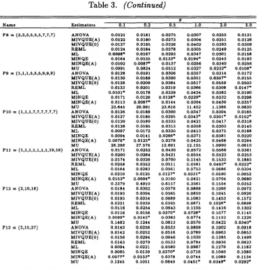
Table 3. Estimated MSE of Estimators ofp

9

Name Estima.tors 0.1 0.2 0.5 1.0 2.0 5.0

Ph=(3,5,7) ANOVA 0.0309 0.0414 0.0655 0.0905 0.1046 0.0908

MIVQUE(A) 0.0312 0.0416 0.0651 0.0902 0.1044 0.0904

MIVQUE(O) 0.0313 0.0425 0.0705 0.0985 0.1178 0.1090

REML 0.0316 0.0423 0.0659 0.0909 0.1046 0.0903

ML 0.0173 0.0305 0.0671 0.1094 0.1386 0.1273

MINQE 0.0188 0.0214 0.0380* 0.0690 0.1001 0.1069

MINQE(A) 0.0138* 0.0178* 0.0399 0.0780 0.1154 0.1234

MU 0.1563 0.1307 0.0781 0.0493* 0.0379* 0.0327*

P2=(1,5,9) ANOVA 0.0353 0.0452 0.0713 0.1010 0.1220 0.1095

MIVQUE(A) 0.0377 0.0468 0.0699 0.1001 0.1217 0.1079

MIVQUE(O) 0.0331 0.0457 0.0820 0.1228 0.1629 0.1758

REML 0.0411 0.0516 0.0761 0.1064 0.1258 0.1087

ML 0.0200 0.0346 0.0778 0.1322 0.1729 0.1616

MINQE 0.0205 0.0209 0.0378* 0.0743* 0.1156 0.1311

MINQE(A) 0.0160* 0.0183* 0.0407 0.0840 0.1309 0.1464

MU 0.2892 0.2757 0.1955 0.1549 0.1056* 0.0720*

P3=(1,7,7) ANOVA 0.0337 0.0439 0.0705 0.1001 0.1212 0.1091

MIVQUE(A) 0.0362 0.0455 0.0688 0.0993* 0.1209 0.1074

MIVQUE(O) 0.0319 0.0448 0.0815 0.1225 0.1634 0.1780

REML 0.0400 0.0507 0.0753 0.1055 0.1248 0.1079

ML 0.0193 0.0338 0.0763 0.1300 0.1699 0.1591

MINQE 0.0199 0.0294 0.0608 0.1046 0.1420 0.1390

MINQE(A) 0.0167* 0.0264* 0.0604* 0.1091 0.1521 0.1523

MU 0.2977 0.2777 0.2085 0.1453 0.1043* 0.0701*

P4=(3,3,5,5,7,7) ANOVA 0.0172 0.0247 0.0394 0.0459 0.0436 0.0258

MIVQUE(A) 0.0173 0.0245 0.0392 0.0458 0.0432 0.0252

MIVQUE(O) 0.0178 0.0266 0.0447 0.0565 0.0608 0.0475

REML 0.0176 0.0251 0.0399 0.0461 0.0431 0.0250

ML 0.0126 0.0215 0.0417 0.0538 0.0542 0.0333

MINQE 0.0174 0.0155 0.0200* 0.0303* 0.0399 0.0340

MINQE(A) 0.0115* 0.0111* 0.0209 0.0376 0.0518 0.0433

MU 0.1090 0.0874 0.0536 0.0378 0.0295* 0.0181 *

P5=(1,1,5,5,9,9) ANOVA 0.0184 0.0263 0.0430 0.0527 0.0535 0.0337

MIVQUE(A) 0.0191 0.0265 0.0422 0.0522 0.0530 0.0319

MIVQUE(O) 0.0182 0.0286 0.0521 0.0723 0.0859 0.0781

REML 0.0201 0.0286 0.0457 0.0552 0.0538 0.0309*

ML 0.0134 0.0235 0.0480 0.0659 0.0697 0.0427

MINQE 0.0184 0.0147 0.0195* 0.0344* 0.0512* 0.0484

MINQE(A) 0.0129* 0.0111* 0.0216 0.0429 0.0637 0.0572

MU 107.70 32.286 26.687 10.332 5.5942 0.1540

P6=(1,1,7,7,7,7) ANOVA 0.0176 0.0259 0.0412 0.0531 0.0527 0.0331

MIVQUE(A) 0.0179 0.0261 0.0403 0.0523* 0.0525* 0.0317

MIVQUE(O) 0.0169 0.0267 0.0464 0.0639 0.0725 0.0619

REML 0.0186 0.0280 0.0436 0.0552 0.0536 0.0310*

ML 0.0123 0.0230 0.0460 0.0658 0.0692 0.0426

MINQE 0.0122 0.0190 0.0365* 0.0561 0.0637 0.0437

MINQE(A) 0.0100* 0.0169* 0.0372 0.0616 0.0732 0.0527

MU 40.027 151.61 79.728 255.58 4.7196 0.5201

P7=(1,1,1,1,13,13) ANOVA 0.0223 0.0307 0.0515 0.0678 0.0753 0.0501

MIVQUE(A) 0.0258 0.0323 0.0504 0.0672 0.0731 0.0438

MIVQUE(O) 0.0212 0.0360 0.0741 0.1164 0.1599 0.1816

REML 0.0312 0.0406 0.0606 0.0727 0.0719 0.0400*

ML 0.0183 0.0305 0.0643 0.0929 0.1022 0.0602

MINQE 0.0208 0.0145 0.0193* 0.0415* 0.0703* 0.0747

MINQE(A) 0.0155* 0.0116* 0.0226 0.0510 0.0832 0.0817

MU 1.4652 2.3543 2.9181 1.2688 0.9073 0.1671

..

Table 3. (Continued)

9

Na.me EI&ima&ofl5 0.1 0.2 0.5 1.0 2.0 5.0

pa=(3,3,3,5,5,5,7,7,7) ANOVA 0.0121 0.0181 0.0275 0.0307 0.0255 0.0131

MIVQUE(A) 0.0122 0.0180 0.0273 0.0304 0.0251 0.0126

MIVQUE(O) 0.0127 0.0195 0.0326 0.0402 0.0393 0.0309

REML 0.0124 0.0184 0.0278 0.0305 0.0249 0.0125

ML 0.0098* 0.0167 0.0293 0.0347 0.0301 0.0158

MINQE 0.0164 0.0135 0.0133* 0.0194* 0.0243 0.0193

MINQE(A) 0.0102 0.0087* 0.0137 0.0256 0.0340 0.0256

MU 0.0991 0.0824 0.0512 0.0327 0.0232* 0.0108*

P9=(1,1,1,5,5,5,9,9,9) ANOVA 0.0128 0.0191 0.0306 0.0357 0.0314 0.0172

MIVQUE(A) 0.0130 0.0189 0.0300 0.0351 0.0307* 0.0155

MIVQUE(O) 0.0128 0.0209 0.0384 0.0517 0.0559 0.0503

REML 0.0133 0.0201 0.0319 0.0366 0.0308 0.0147*

ML 0.0101* 0.0178 0.0339 0.0424 0.0382 0.0190

MINQE 0.0171 0.0126 0.0128* 0.0229* 0.0332 0.0298

MINQE(A) 0.0113 0.0087* 0.0144 0.0304 0.0439 0.0357

MU 23.645 30.991 23.616 11.452 1.1366 0.0630

P10=(1,1,1,7,7,7,7,7,7) ANOVA 0.0126 0.0188 0.0300 0.0347 0.0304 0.0165

MIVQUE(A) 0.0127 0.0186 0.0295 0.0343* 0.0301* 0.0152*

MIVQUE(O) 0.0120 0.0189 0.0333 0.0421 0.0417 0.0318

REML 0.0128 0.0195 0.0313 0.0358 0.0303 0.0145

ML 0.0097 0.0172 0.0330 0.0413 0.0375 0.0188

MINQE 0.0094 0.0141 0.0266* 0.0371 0.0381 0.0220

MINQE(A) 0.0076* 0.0125* 0.0278 0.0425 0.0468 0.0284

MU 28.266 27.576 12.691 12.155 1.0990 0.0610

PI1= (1,1,1,1,1,1,1,19,19) ANOVA 0.0171 0.0252 0.0430 0.0572 0.0568 0.0361

MIVQUE(A) 0.0200 0.0264 0.0421 0.0554 0.0523 0.0253

MIVQUE(O) 0.0174 0.0326 0.0700 0.1145 0.1533 0.1885

REML 0.0258 0.0352 0.0511 0.0581 0.0493* 0.0222*

ML 0.0164 0.0283 0.0561 0.0753 0.0686 0.0304

MINQE 0.0210 0.0125 0.0127* 0.0331* 0.0590 0.0652

MINQE(A) 0.0152* 0.0094* 0.0160 0.0421 0.0704 0.0680

MU 0.3379 0.4910 0.6157 0.3561 0.1554 0.0352

P12=(2,10,18) ANOVA 0.0184 0.0302 0.0579 0.0868 0.1066 0.0972

MIVQUE(A) 0.0193 0.0304 0.0565 0.0859 0.1045 0.0926

MIVQUE(O) 0.0193 0.0334 0.0689 0.1083 0.1453 0.1572

REML 0.0221 0.0339 0.0595 0.0871 0.1028* 0.0898

ML 0.0116 0.0254 0.0643 0.1105 0.1416 0.1302

MINQE 0.0116 0.0156 0.0370* 0.0728* 0.1077 0.1145

MINQE(A) 0.0099* 0.0145* 0.0383 0.0774 0.1152 0.1226

MU 0.1482 0.1244 0.0813 0.0576 0.0422 0.0340*

P13=(3,15,27) ANOVA 0.0140 0.0256 0.0533 0.0809 0.1002 0.0918

MIVQUE(A) 0.0142 0.0252 0.0516 0.0789 0.0963 0.0853

MIVQUE(O) 0.0156 0.0294 0.0646 0.1030 0.1385 0.1499

REML 0.0163 0.0279 0.0533 0.0784 0.0936 0.0823

ML 0.0094 0.0221 0.0580 0.0987 0.1276 0.1182

MINQE 0.0085 0.0139 0.0370* 0.0716 0.1040 0.1080

MINQE(A) 0.0077* 0.0133* 0.0378 0.0744 0.1089 0.1134

MU 0.1245 0.1051 0.0649 0.0451* 0.0348* 0.0292*

..

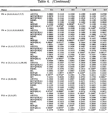
Table 4. Estimated Absolute Bias Estimators of p

8

Na.me Es\ima.t.ors 0.1 0.2 0.5 1.0 2.0 5.0

P1=(3,5,1) ANOVA 0.1314 0.1696 0.22(6 0.2535 0.2509 0.2019

MIVQUE(A) 0.1314 0.1693 0.22(0 0.253( 0.2501 0.2008

MIVQUE(O) 0.1303 0.1100 0.2315 0.2661 0.2158 0.2H5

REML 0.1326 0.1114 0.2251 0.25(0 0.2505 0.2003

ML 0.1058 0.15U 0.2311 0.2825 0.2955 0.2511

MINQE 0.0916 0.1141 0.1613· 0.2211 0.2535 0.2(21

MINQE(A) 0.0837· 0.1071· 0.173( 0.2388 0.2196 0.2681

MU 0.3136 0.3311 0.2290 0.1806· 0.1591· 0.1212·

P2 = (1,5,9) ANOVA 0.139( 0.1119 0.2366 0.2712 0.2150 0.2267

MIVQUE(A) 0.1416 0.1111 0.2330 0.2103 0.2H1 0.222(

MIVQUE(O) 0.1321 0.1110 0.2565 0.3088 0.3319 0.3211

REML 0.1457 0.1880 0.2(61 0.2793 0.2162 0.2181

ML 0.1099 0.16(5 0.2558 0.3183 0.335( 0.28U

MINQE 0.1026 O.l1U 0.1612· 0.2314· 0.2191 0.28(6

MINQE(A) 0.0895· 0.1083· 0.1757 0.2506 0.30(5 0.3031

MU 0.(613 0.(225 0.3091 0.U51 0.1975· 0.H59·

P3 = (1,7,7) ANOVA 0.1365 0.1151 0.23H 0.2699 0.2H5 0.2210

MIVQUE(A) 0.1388 0.1750 0.2310 0.2691 0.21M 0.2222

MIVQUE(O) 0.1301 0.1152 0.2553 0.3082 0.3381 0.32(0

REML 0.1435 0.1860 0.2(50 0.2119 0.2H9 0.2180

ML 0.1079 0.1619 0.2526 0.3153 0.3325 0.282'

MINQE 0.1071 0.lU9 0.2181· 0.21U 0.3059 0.2721

MINQE(A) 0.0993· 0.1390· 0.2181 0.2866 0.3216 0.2922

MU 0.(6(8 0.(236 0.31U 0.2UO· 0.1969· 0.1453·

P. = (3,3,5,5,7,7) ANOVA 0.1032 0.1314 0.166' 0.1720 0.1566 0.1070

MIVQUE(A) 0.1028 0.1303 0.1659 0.1716 0.15M 0.1051

MIVQUE(O) 0.1032 0.13(0 0.1766 0.1939 0.1951 0.1681

REML 0.10U 0.1325 0.1675 0.1719 0.lM9 0.10H

ML 0.092( 0.12H 0.1719 0.1852 0.113' 0.1217

MINQE 0.1001 0.095( 0.1166· O.HO.· 0.1538 0.1329

MINQE(A) 0.0788· 0.0816· 0.1202 0.1587 0.1806 0.1532

MU 0.3161 0.2109 0.1713 0.H17 0.1285· 0.092(·

P5 = (1,1,5,5,9,9) ANOVA 0.1062 0.1351 0.1151 0.1856 0.lH1 0.1225

MIVQUE(A) 0.1065 0.13U 0.1729 0.18U 0.1716 0.116(

MIVQUE(O) 0.1032 0.138( 0.1928 0.2225 0.2355 0.215'

REML 0.1080 0.140( 0.1814 0.1896 0.1711· 0.1131·

ML 0.093( 0.1331 0.1812 0.2012 0.1956 0.1338

MINQE 0.1036 0.093( 0.1151· 0.1506· 0.1796 0.1686

MINQE(A) 0.0831· 0.0819· 0.1226 0.1717 0.2056 0.1831

MU 1. 7565 1.3908 0.9003 0.5050 0.2857 0.lH1

P6 = (1,1,7,7,1,7) ANOVA 0.10(6 0.13'6 0.1709 0.1863 0.1736 0.1215

MIVQUE(A) 0.10(0 0.1333 0.1685 0.18U· 0.1716· 0.1163

MIVQUE(O) 0.1013 0.1361 0.1821 0.2081 0.2099 0.1110

REML 0.10H 0.1381 0.1166 0.1891 0.1716· 0.1131·

ML 0.0905 0.1301 0.1836 0.2075 0.1955 0.13(5

MINQE 0.0883 0.1151 0.1608· 0.1930 0.1937 0.H36

MINQE(A) 0.0806· 0.1099· 0.1639 0.20(9 0.2116 0.1621

MU 1.6783 1. 7167 1.0851 0.730' 0.2891 0.1193

P7 = (1,1,1,1,13,13) ANOVA 0.1155 0.H68 0.19(2 0.2135 0.2120 0.15(2

MIVQUE(A) 0.1201 0.H67 0.19H 0.2131 0.203( 0.13U

MIVQUE(O) 0.1091 0.1561 0.2(01 0.2999 0.3(16 0.3(36

REML 0.1291 0.1683 0.2141 0.2191 0.195(· 0.12(2·

ML 0.10(0 0.1531 0.2253 0.2511 0.2363 0.1535

MINQE 0.1122 0.0931 0.lH9· 0.1692· 0.2221 0.2282

MINQE(A) 0.0929· 0.083(· 0.1265 0.1922 0.2U1 0.2325

MU 0.6(65 0.6M6 0.5317 0.3655 0.2(99 0.1211

Table 4. (Continued)

(J

Na.me E.,imatollJ 0.1 0.2 0.5 1.0 2.0 5.0

P8=(3,3,3,5,5,5,7,7,7) ANOVA 0.0883 0.1118 0.1358 0.1389 0.1209 0.0789

MIVQUE(A) 0.0879 0.1110 0.13M 0.1383 0.1194 0.0771

MIVQUE(O) 0.0891 0.1144 0.1480 0.1618 0.1575 0.1381

REML 0.0889 0.1128 0.1366 0.1384 0.1190 0.0769

ML 0.0822 0.1100 0.1406 0.1465 0.1295 0.0858

MINQE 0.1029 0.0903 0.0938· 0.1117· 0.1196 0.1024

MINQE(A) 0.0777· 0.0718· 0.0965 0.1303 0.1462 0.1197

MU 0.3015 0.2582 0.1529 0.1243 0.1108· 0.0725·

P9=(1,1,1,5,5,5,9,9,9) ANOVA 0.0906 0.1152 0.1440 0.1507 0.1341 0.0900

MIVQUE(A) 0.0901 0.1130 0.1424 0.1488 0.1309 0.0837

MIVQUE(O) 0.0890 0.1180 0.1623 0.1862 0.1896 0.1762

REML 0.0909 0.1170 0.1475 0.1516 0.1301· 0.0814·

ML 0.0829 0.1134 0.1528 0.1626 0.1437 0.0920

MINQE 0.1059 0.0876 0.0921· 0.1221· 0.1443 0.1352

MINQE(A) 0.0824· 0.0717· 0.0994 0.1440 0.1708 0.1471

MU 1.9331 1.9227 1.1026 0.5394 0.1983 0.0818 PI0=(1.1.1.7.7.7.7.7.7) ANOVA 0.0899 0.1144 0.1426 0.1487 0.1319 0.0878

MIVQUE(A) 0.0892 0.1124 0.1411 0.1471 0.1297 0.0833

MIVQUE(O) 0.0878 0.1135 0.1512 0.1661 0.1578 0.1274

REML 0.0895 0.1152 0.1458 0.1502· 0.1294· 0.0811·

ML 0.0816 0.1113 0.1504 0.1607 0.1427 0.0916

MINQE 0.0780 0.0983 0.1343· 0.1547 0.1486 0.1021

MINQE(A) 0.0707· 0.0935· 0.1390 0.1679 0.1680 0.1193

MU 2.0320 1.8656 1.0563 0.5683 0.2066 0.0814 Pll =(1.1.1.1.1.1.1.19.19) ANOVA 0.1032 0.1327 0.1747 0.1959 0.1848 0.1352

MIVQUE(A) 0.1071 0.1313 0.1740 0.1912 0.1689 0.1018

MIVQUE(O) 0.1002 0.1493 0.2320 0.2987 0.3343 0.3561

REML 0.1191 0.1576 0.1941 0.1912 0.1580· 0.0933

ML 0.0994 0.1467 0.2067 0.2192 0.1853 0.1081

MINQE 0.1201 0.0877 0.0927· 0.1526· 0.2104 0.2250

MINQE(A) 0.0977· 0.0744· 0.1061 0.1765 0.2311 0.2217

MU 0.4333 0.4529 0.3822 0.2702 0.1732 0.0891· P12=(2.10.18) ANOVA 0.1056 0.1469 0.2097 0.2485 0.2564 0.2152

MIVQUE(A) 0.1059 0.1458 0.2071 0.2471 0.2511 0.2044

MIVQUE(O) 0.1067 0.1540 0.2328 0.2865 0.3173 0.3042

REML 0.1129 0.1556 0.2133 0.2472 0.2463 0.1989

ML 0.0915 0.1446 0.2262 0.2833 0.2984 0.2541

MINQE 0.0783 0.1021 0.1657· 0.2284 0.2665 0.2550

MINQE(A) 0.0732· 0.0999· 0.1697 0.2374 0.2790 0.2671

MU 0.3646 0.3253 0.2315 0.1856· 0.1588· 0.1257· P13=(3.15.27) ANOVA 0.0936 0.1346 0.2000 0.2394 0.2487 0.2101

MIVQUE(A) 0.0930 0.1335 0.1969 0.2346 0.2398 0.1963

MIVQUE(O) 0.0970 0.1445 0.2245 0.2796 0.3090 0.2971

REML 0.0999 0.1412 0.1998 0.2321 0.2344 0.1914

ML 0.0849 0.1344 0.2122 0.2642 0.2820 0.2435

MINQE 0.0695 0.0981 0.1656· 0.2251 0.2602 0.2443

MINQE(A) 0.0668· 0.0970· 0.1681 0.2310 0.2685 0.2529

MU 0.3378 0.3033 0.2097 0.1701· 0.1499· 0.1211·

Table 5. MSE of Four Estimators of ()

e

Name Estimators 0.1 0.5 1.0 5.0

PB

=

(5,5,5,5,5,5,5,5,5) ML 0.02 0.14 0.42 7.95 MINQE 0.02 0.13 0.45 9.46 MINQE(A) 0.01· 0.01· 0.24· 6.35·

PM 0.01· 0.10 0.30 6.38

P8

=

(3,3,3,5,5,5,7,7,7) ML 0.02 0.14 0.45 7.95 MINQE 0.02 0.13 0.45 9.34 MINQE(A) 0.01· 0.10· 0.35 1.33 PM 0.01· 0.10· 0.30· 6.13· PH

=

(1,1,1,1,1,1,1,19,19) ML 0.06 0.35 0.88 9.60 MINQE 0.02 0.14 0.48 9.18 MINQE(A) 0.01· 0.13· 0.44· 9.03

PM 0.02 0.15 0.48 8.49·

• means the best choice.

Table 6. Bias of Four Estimators of ()

e

Name Estimators 0.1 0.5 1.0 5.0

PB

=

(5,5,5,5,5,5,5,5,5) ML -0.01· -0.04 -0.01 -0.30 MINQE 0.03 0.00· -0.02· -0.01· MINQE(A) 0.09 -0.04 -0.21 -1.60

PM -0.02 -0.14 -0.39 -1.70

P8

=

(3,3,3,5,5,5,7,1,7) ML 0.00· -0.04 -0.01 -0.31

MINQE 0.03 -0.01· -0.05· -0.08· MINQE(A) 0.01 -0.09 -0.21 -0.89

PM -0.02 -0.14 -0.30 -1.72

Pll

=

(1,1,1,1,1,1,1,19,19) ML 0.00· -0.04· -0.05· -0.30· MINQE 0.00· -0.16 -0.36 -1.67 MINQE(A) 0.00· -0.20 -0.44 -2.00

PM -0.03 -0.24 -0.46 -2.00

..

Table 7. MSE of Four Estimators of p

8

Name Estimators 0.1 0.2 0.5 1.0 2.0 5.0

Pl-(3,5,7) ML 0.0173 0.0305 0.0671 0.1094 0.1386 0.1273

MINQE 0.0188 0.0214 0.0380* 0.0690 0.1001 0.1069

MINQE(A) 0.0138* 0.0178* 0.0399 0.0780 0.1154 0.1234

MEDIAN 0.0263 0.0271 0.0416 0.0655* 0.0970* 0.0914*

P2

=

(1,5,9) ML 0.0200 0.0346 0.0778 0.1322 0.1729 0.1616

MINQE 0.0205 0.0209 0.0378* 0.0743 0.1156 0.1311

MINQE(A) 0.0160* 0.0183* 0.0407 0.0840 0.1309 0.1464

MEDIAN 0.0665 0.0571 0.0495 0.0622* 0.0778* 0.0830*

P3

=

(1,7,7) ML 0.0193 0.0338 0.0763 0.1300 0.1699 0.1591

MINQE 0.0199 0.0294 0.0608 0.1046 0.1420 0.1390

MINQE(A) 0.0167* 0.0264* 0.0604 0.1091 0.1521 0.1523

MEDIAN 0.0611 0.0584 0.0530* 0.0597* 0.0831* 0.0853* P4

=

(3,3,5,5,7,7) ML 0.0126 0.0215 0.0417 0.0538 0.0542 0.0333

MINQE 0.0174 0.0155 0.0200* 0.0303 0.0399 0.0340

MINQE(A) 0.0115* 0.0111* 0.0209 0.0376 0.0518 0.0433

MEDIAN 0.0298 0.0258 0.0234 0.0284* 0.0300* 0.0223* P5

=

(1,1,5,5,9,9) ML 0.0134 0.0235 0.0480 0.0659 0.0697 0.0427

MINQE 0.0184 0.0147 0.0195* 0.0344 0.0512 0.0484

MINQE(A) 0.0129* 0.0111* 0.0216 0.0429 0.0637 0.0572

MEDIAN 0.0722 0.0576 0.0375 0.0296* 0.0273* 0.0180* P6

=

(1,1,7,7,7,7) ML 0.0123 0.0230 0.0460 0.0658 0.0692 0.0426

MINQE 0.0122 0.0190 0.0365 0.0561 0.0637 0.0437

MINQE(A) 0.0100* 0.0169* 0.0372 0.0616 0.0732 0.0527

MEDIAN 0.0720 0.0608 0.0341* 0.0303* 0.0259* 0.0218* P7

=

(1,1,1,1,13,13) ML 0.0183 0.0305 0.0643 0.0929 0.1022 0.0602

MINQE 0.0208 0.0145 0.0193* 0.0415 0.0703 0.0747

MINQE(A) 0.0155* 0.0116* 0.0226 0.0510 0.0832 0.0817

MEDIAN 0.1282 0.0995 0.0558 0.0366* 0.0240* 0.0156* P8

=

(3,3,3,5,5,5,7,7,7) ML 0.0098* 0.0167 0.0293 0.0347 0.0301 0.0158

MINQE 0.0164 0.0135 0.0133* 0.0194 0.0243 0.0193

MINQE(A) 0.0102 0.0087* 0.0137 0.0256 0.0340 0.0256

MEDIAN 0.0272 0.0269 0.0191 0.0184* 0.0172* 0.0096* P9

=

(1,1,1,5,5,5,9,9,9) ML 0.0101* 0.0178 0.0339 0.0424 0.0382 0.0190

MINQE 0.0171 0.0126 0.0128* 0.0229 0.0332 0.0298

MINQE(A) 0.0113 0.0087* 0.0144 0.0304 0.0439 0.0357

MEDIAN 0.0774 0.0616 0.0351 0.0220* 0.0168* 0.0086* PI0

=

(1,1,1,7,7,7,7,7,7) ML 0.0097 0.0172 0.0330 0.0413 0.0375 0.0188

MINQE 0.0094 0.0141 0.0266* 0.0371 0.0381 0.0220

MINQE(A) 0.0076* 0.0125* 0.0278 0.0425 0.0468 0.0284

MEDIAN 0.0723 0.0569 0.0329 0.0215* 0.0159* 0.0083* P11

=

(1,1,1,1,1,1,1,19,19) ML 0.0164 0.0283 0.0561 0.0753 0.0686 0.0304

MINQE 0.0210 0.0125 0.0127* 0.0331* 0.0590 0.0652

MINQE(A) 0.0152* 0.0094* 0.0160 0.0421 0.0704 0.0680

MEDIAN 0.1593 0.1214 0.0674 0.0369 0.0172* 0.0061* P12

=

(2,10,18) ML 0.0116 0.0254 0.0643 0.1105 0.1416 0.1302

MINQE 0.0116 0.0156 0.0370* 0.0728 0.1077 0.1145

MINQE(A) 0.0099* 0.0145* 0.0383 0.0774 0.1152 0.1226

MEDIAN 0.0253 0.0274 0.0401 0.0634* 0.0829* 0.0843* P13

=

(3,15,27) ML 0.0094 0.0221 0.0580 0.0987 0.1276 0.1182

MINQE 0.0085 0.0139 0.0370 0.0716 0.1040 0.1080

MINQE(A) 0.0077* 0.0133* 0.0378 0.0744 0.1089 0.1134

•

P2 and 0

=

5.0 under P3 in the sense of MSE criterion. Similarly,

MIVQUE(A) has smaller absolute bias than REML estimators except

o=

5.0 under PH and 0

=

5.0 under P13.

5. The MU estimator has poor efficiency for any values ofkandO.MU has

highest absolute bias and smallest MSE efficiency except MIVQUE(O).

3.2

Estimation of

p

It is difficult to obtain good estimator of intraclass correlation coefficient p under MSE and absolute bias criterion. However, one possibility is to find

the approximation for MSE ofg(X), whereg(X) means that the estimator of

intraclass correlation coefficientg(O)

=

0/(1

+

0). Ifwe expand9 in a Taylor series, keeping only to one term, then E(g(X) - g(O))2":'[g'(O)]2E(X _ 0)2.

This means that good estimator of 0 is also desirable estimator of

g(

0),

approximately. But it is not easy to improve this approximation by using

higher-order moments ofX.

To draw general conclusions for the estimation of intraclass correlation coefficient p,a simulation study was performed using the procedure described in section 3. The results of the simulations are shown in Table 3 and Table 4. The following conclusions are drawn from all the computed values.

1. For all around performance except P8 and P9 designs, the MINQE(A)

estimator of the p may have smaller MSE than any other estimator if

o::;

0.2. In the case of absolute bias, MINQE(A) is the best estimator

when 0 ::; 0.2. MINQE performs very well if 0

=

0.5 and 0

=

1.0. However, the best winner in the sense of MSE and absolute bias is not clear. Because the difference of efficiency to their performances is very small.

2. The MU estimator of p performs well if the value of k is small and 0

is thought to be large. However when 0 ::; 0.5, the MU estimators is a

terrible estimator ofp.

3. The ANOVA, MIVQUE(A) and REML estimators of p have similar efficiency. Further iteration to the REML estimates is unnecessary for the estimation ofp.

5. The MIVQUE(O) is a poor estimator for p when

e

is large. The MIVQUE(O) is a desirable estimator only when one is confident that

e

~ O.

4

Comparisons of Other Procedures

4.1

Attention on Point estimation of

e.

Several other estimators of

e

have also been cited in the literature. Chaloner

(1987) used the bayesian posterior mode estimator of

e

in the consideration

of estimation of

e.

In his paper, the posterior mode estimator (PME) is

superior to MLE. We reproduced a table regarding the efficiencies of MLE, PME, and two types of MINQE. Table 5 illustrates MSE and average bias of

four estimators of

e.

The values of MSE and bias for ML and PM estimators

were duplicated in Chaloner (1987) except the case of design PB. MSE and average bias of ML and MINQE(A), respectively, can be calculated exactly when the data is balanced. By this reason, we used the exact values of MSE and bias at Table 5 and Table 6. Table 5 illustrates the following points:

1. The MSE of the MINQE(A) is less than the MSE of any other estimator

for

e :::;

0.5.

2. Irrespective of small MSE of MINQE(A) and PME, they may have a nontrivial bias. Moreover, the absolute value of bias for PM is large

than that of MINQE(A) except

e

= 0.1 undere PB.

3. Every estimators are generally biased downward for

e:::;

0.5.

4. PME is not generally much more efficient than the MINQE(A). Of course, the expense of computation for PME is very high, although the MINQE(A) can be easily computed by hand.

4.2

Attention on Point estimation of

p.

Palmer and Broemeling (1990) pointed out the possibility of using the Bayes estimator used the median of a conditional posterior density as its estimator

of p. We reproduced a table regarding to the efficiencies of MLE, PME,

estimators of O. Again the values for the Bayes estimators are taken from the Monte Carlo study of Palmer and Broemeling (1990). Table 7 gives the MSE and bias for four estimators. The MSE of the Bayes estimator is less

than the MSE of any other estimators for p ~ 1.0. Ifp :::; 0.2 then MSE of

MINQE(A) is the smallest except Pl1. MINQE is the best around p

=

0.5

approximately.

5

Summary and Conclusions

To sum up, we recommend the followings:

1. For estimating of 0, two types of MINQE estimators seem to be the best or nearly best estimators unless the value of () is thought to be

high. For low values of0it is recommended that MINQE(A) be used.

2. For estimating ofp, the MINQE(A) estimators seems to be the overall

best choice in the case of p :::; 0.2. When the value of p ~ 1.0, the Bayes median estimates of p is recommended.

References

[1] Ahrens, H., Kleffe,

J.,

and Tenzler, R. (1981). "Mean Square Error Com-parison for MINQUE, ANOVA and Two Alternative Estimators Under the Unbalanced One-Way Random Model," Biomedical Journal, Vol. 23, 323 - 342.

[2] Burdick, R. K., Maqsood, F., and Graybill, F. A. (1986). "Confidence Intervals on the Intraclass Correlation in the Unbalanced One-Way Clas-sification," Commun. Statist.- Theor. Meth., Vol. 15, 3353 - 3378.

[3] Chaloner, K. (1987). "A Bayesian Approach to the Estimation of Vari-ance Components for the UnbalVari-anced One Way Random Model,"

Tech-nometrics, Vol. 29(3), 323 - 337.

[4] Conerly, M. D., and Webster, J. T. (1987). "MINQE for the One-Way

•

[5] Das, K. (1992). "Improved Estimation of the Ratio of Variance

Com-ponents for a Balanced One-Way Random Effects Model," Statistics (3

Probability Letters, Vol. 13, 99 - 108.

[6] Donner, A., and Koval, J. J. (1986). "The Estimation of Intraclass Cor-relation in the Analysis of Family Data," Biometrics, Vol. 36, 19 - 25.

[7] Donner, A., and Wells, G. (1986). "A Comparison of Confidence Interval Methods for the Intraclass Correlation Coefficient," Biometrics, Vol. 42, 401 - 412.

[8] Loh, Wei-Yin. (1986). "Improved Estimators for Ratios of Variance Components;" Journal of the American Statistical Association, Vol. 81, 699 - 702.

[9] Lee, J. T., and Lee, K. S. (1990). "A Comparison on Non-Negative Estimators for Ratios of Variance Components," Proc. COMSTAT'90, 303 - 308.

[10] Palmer, J. 1., and Broemeling, 1. D. (1990). "A Comparison of Bayes

and Maximum Likelihood Estimation of the Intraclass Correlation Co-efficient," Commun. Statist.- Theor. Meth., Vol. 19(3), 953 - 975.

[11] Rao, P. S. R. S., and Chaubey, Y. P. (1978). "Three Modifications of the principle of MINQUE," Commun. Statist.- Theor. Meth., Vol. A7(8),

767 - 778.

[12] Rao, C. R. (1971). "Minimum Variance Quadratic Unbiased Estimation of Variance Components," Journal of Multivariate Analysis, Vol. 1, 445 - 456.

[13] Rao, C. R., and Kleffe, J. (1988). Estimation of Variance Components

and Applications, North-Holland, Amsterdam.

[14] Searle, S. R. (1971). Linear Models, New York: John Wiley.

•

•

[16] Swallow, W. H., and Searle, S. R. (1978). "Minimum Variance Quadratic Unbiased Estimation (MIVQUE) of Variance Components,"

Technomet-rics, Vol. 20, 265 - 272.

[17] Wald, A. (1940). "A Note on the Analysis of Variance With Unequal Class Frequencies," Annals of Mathematical Statistics, Vol. 11, 96 -100.