ABSTRACT
HEGDE, AMRUTHKIRAN. Experimental Investigation into Shock Induced Corner Boundary Layer Separation. (Under the direction of Dr.Venkateswaran Narayanaswamy).
Experimental Investigation into Shock Induced Corner Boundary Layer Separation
by
Amruthkiran Hegde
A thesis submitted to the Graduate Faculty of North Carolina State University
in partial fulfillment of the requirements for the degree of
Master of Science
Aerospace Engineering
Raleigh, North Carolina 2015
APPROVED BY:
_______________________________ ______________________________ Dr.Hong Luo Dr.Hassan Hassan
Committee Member Committee Member
ACKNOWLEDGMENTS
TABLE OF CONTENTS
LIST OF TABLES……….v
LIST OF FIGURES ... vi
CHAPTER-1. INTRODUCTION TO SHOCK WAVE/TURBULENT BOUNDARY LAYER INTERACTION………. 1
CHAPTER-2. A REVIEW OF PAST RESEARCH AND MECHANISM OF SBLI……….. 4
2.1. Centerline Flow………. . 4
2.2 Corner Flow………... 8
CHAPTER-3. RESEARCH MOTIVATION………...12
CHAPTER-4. EXPERIMENTAL FACILITY DESIGN AND ASSISTING SET UPS ... 13
4.1 Wind Tunnel Design ………..13
4.2 Schlieren Imaging ………..13
4.3 Surface Flow Visualization ... 15
4.4 Unsteady Pressure Measurements ... 15
4.5 Auxiliary Experimental Set up... 16
CHAPTER-5. FLAT PLATE BOUNDARY LAYER MEASUREMENT ... 18
5.1 Experimental Setup ... 18
5.2 Experimental procedure ... 20
5.3 Results and Discussion ... 24
CHAPTER-6. SBLI IN EXPERIMENTAL SET-UP ... 24
6.1 Incident shock reflection method ... 25
6.1.1. Experimental Setup ... 25
6.1.2. Surface Flow Visualization ... 26
6.1.3. Schlieren Imaging ... 27
6.2 Flow Separation by compression ramp ... 28
6.2.1 Experimental setup... 28
6.2.2. Baseline Flow... 29
6.2.3.2 Surface Flow Visualization with 12o ramp (Mach 3.3)………...36
6.2.3.3 Surface Flow Visualization with 16o ramp (Mach 2.5)……….37
6.2.3.4 Surface Flow Visualization with 16o ramp (Mach 3.3)……….41
6.2.4 Static Pressure Measurements………. 43
CHAPTER-7. SUMMARY AND FUTURE WORK………...57
REFERENCES………... 59
LIST OF TABLES
LIST OF FIGURES
Figure 1. Image of Rectangular to Elliptic Shape Transition Inlet (REST)……….. 2
Figure 2. Schematic of wave pattern in a compression corner (from Vishwanath 1988)…... 5
Figure 3. Schematic of wave pattern without separation (a) compression corner (b) incident shock (from Vishwanath 1988)………. 5
Figure 4. The three canonical geometries depicting SBLI (a) compression corner (b) incident shock (c) blunt fin (from Clemens et al. 2013)………. 7
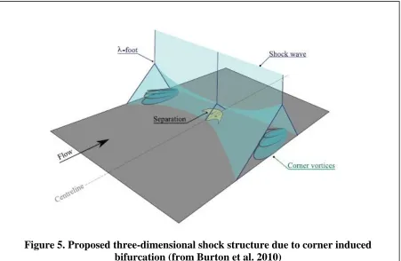
Figure 5. Proposed three-dimensional shock structure due to corner induced bifurcation (from Burton et al. 2010)………11
Figure 6. Schlieren Setup………..14
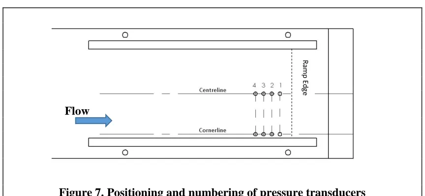
Figure 7. Positioning and numbering of the pressure transducers………...16
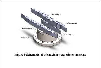
Figure 8.Schematic of the auxiliary set up………17
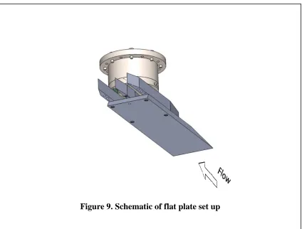
Figure 9.Schematic of flat plate set up………..19
Figure 10. A view of the flat plate set up in the wind tunnel………..20
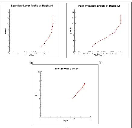
Figure 11. (a) boundary layer profile at Mach 2.5 (b)pitot pressure profile at Mach 2.5 (b) u+ Vs y+ at Mach 2.5………...22
Figure 12. (a) boundary layer profile at Mach 3.3 (b)pitot pressure profile at Mach 3.3 (b) u+ Vs ln y+ at Mach 3.3………...23
Figure 13.Schematic of corner flow………...26
Figure 14.Flow Visualization by incident shock method………...27
Figure 16. (a) flow at Mach 2.5 (b) flow at Mach 3.3………30
Figure 17. Surface Flow Visualization with 12o ramp (Mach 2.5) (a) side view (b) isometric view(c) top view………...33
Figure 18. Top view of Surface Flow Visualization with 12o ramp (Mach 3.3)……….36
Figure 19. Surface Flow Visualization with 16o ramp (Mach 2.5) (a) top view (b) isometric view ( c ) side view………...38
Figure 20. Top view of Surface Flow Visualization with 16o ramp (Mach 3.3)……….41
Figure 21. (a) Avg. Prms/Pwall for Centerline flow at Mach 2.5 (b) Avg. Prms/Pwall for Centerline flow at Mach 3.3 (c) Avg. Prms/Pwall for Corner flow at Mach 2.5 (d)Avg. Prms/Pwall for Corner flow at Mach 3.3………...44
Figure 22. (a) Avg. Pwall/Pinf for Centerline flow at Mach 2.5 (b) Avg. Pwall/Pinf for Centerline flow at Mach 3.3 (c) Avg. Pwall/Pinf for Corner flow at Mach 2.5 (d)Avg. Pwall/Pinf for Corner flow at Mach 3.3………...46
Figure 23. Power Spectral Density for 12o ramp (Centerline flow) at Mach 2.5………...48
Figure 24. Power Spectral Density for 12o ramp (Centerline flow) at Mach 3.3………...49
Figure 25. Power Spectral Density for 16o ramp (Centerline flow) at Mach 2.5………...50
Figure 26. Power Spectral Density for 16o ramp (Centerline flow) at Mach 3.3………...51
Figure 27. Power Spectral Density for 12o ramp (Corner flow) at Mach 2.5……….52
Figure 28. Power Spectral Density for 12o ramp (Corner flow) at Mach 3.3……….53
Figure 29. Power Spectral Density for 16o ramp (Corner flow) at Mach 2.5……….54
CHAPTER-1. INTRODUCTION TO SHOCK WAVE/TURBULENT BOUNDARY LAYER INTERACTION
Shock Wave/Turbulent Boundary Layer Interaction (SBLI) is a common feature and a complex flow phenomena in supersonic jet engine inlets, reaction jets, wings on transonic aircrafts and in experimental facilities such as supersonic wind tunnels.
A large portion of research on SBLI till date has mainly focused only on the centreline flow in SBLIs, away from the corners, without taking the corner effect into consideration and has treated the interaction as a two dimensional interaction. However, streamwise corner flow that forms at the intersection of the walls which enclose the channels is an unavoidable feature in the supersonic jet inlet and experimental facilities. This corner flow which encompasses the boundary layer of both the walls imparts three dimensionality into SBLIs (meaning all the three components of velocity having mean and fluctuations) and hence the SBLIs can seldom be practically treated as 2-D. For e.g., as seen in figure.1, in the REST inlet design in most scramjet vehicles, we observe a change of cross section from rectangular at the inlet to elliptical
CHAPTER-2. A REVIEW OF PAST RESEARCH AND MECHANISM OF SBLI
2.1. Centerline Flow
When a shockwave meets a surface in inviscid flow, it causes an abrupt pressure rise across the surface. However, due to the viscous nature of fluids, a boundary layer always develops near the surface when a fluid flows over a body. Further, in supersonic flow, there is always a region in the boundary layer below which the flow is subsonic. This subsonic flow cannot support an abrupt pressure rise as that caused by the shock wave. Thus the shock wave terminates at the sonic line in the boundary layer (this is called the shock foot) and imparts pressure disturbances which travel both upstream and downstream of the flow. The subsonic stream tubes thicken in reaction to the adverse pressure gradient and generate compression waves which travel in the supersonic part of the boundary layer. These waves cause additional pressure rise and readjustment of the subsonic part of the boundary layer. This cycle continues until there is a compatibility between the gradual pressure rise in the subsonic region of the boundary layer with the abrupt pressure rise in the outer inviscid flow. If the pressure rise is “weak”, then the boundary layer can negotiate the pressure rise without separation. In the case
Figure 2. Schematic of wave pattern in a compression corner (from Vishwanath 1988)
As pressure rise builds with increasing shock strength, the fluid in the boundary layer does not have enough momentum to overcome the adverse pressure gradient imposed by the outer inviscid flow and starts decelerating past the shock wave. The boundary layer eventually separates with the fluid reversing its flow direction. This is the point of incipient flow separation. It is marked with the appearance of separation bubble. The upstream separated boundary layer lifts over the bubble. In the case of a ramp, this deflection leads to the formation of a separation shock. With further increase in the inviscid disturbance, the separation bubble grows in size pushing the separation/reflected shock further upstream. The separation bubble grows as a free shear and acquires kinetic energy as a result of mixing. Once it acquires enough energy, it overcomes the adverse pressure gradient leading to flow reattachment. The lengthscale, Lsep between the flow separation and reattachment is called the length of
separation. This lengthscale keeps varying, as one of the most striking features of the separation bubble is its unsteady breathing motion with fluid entering and emptying it cyclically. The parameters governing this feature is under debate with researchers arguing that both upstream and downstream flow conditions contribute towards its growth and collapse. Also, separation/reflected shock foot oscillates back and forth over a region of Li called the
with increase in Mach number, the shock sweeps larger lengths with lower frequencies due to which the SBLI along the centerline are generally characterized as interactions with low frequency unsteadiness. Figure. 4 shows the schematics of the canonical geometries and the different regions in SBLI.
A bulk of the knowledge on the characteristics of SBLI is from the research that has mainly concentrated on a normal shock turbulent boundary layer interaction, with the parameters governing the condition of flow separation in a normal SBLI being the focus of research over
the time. Principal contributors in this area over the last sixty years include Ackeret, Feldmann & Rott (1947), Seddon (1960), Kooi (1978), Delery (1985) and Sajben et al. (1991). Researchers agree that interaction strength (incoming flow Mach number) is the single most important factor in determining whether a turbulent boundary layer separates or remains attached through a normal SBLI. Factors such as the incompressible boundary layer shape factor ahead of the interaction (Hi0) with the Reynolds number (Re) effect incorporated into it. Bruce et al. (2011) summarized the experiments on SBLIs conducted at different facilities till then. Combining the results from the experiments done previously, they came up with a parameter which is an aspect ratio, 𝛿∗/𝑤 (δ* is the boundary layer displacement thickness and w is the width of the channel) and plotted it against the Mach number thus predicting the separation of flow. The results from the previous experiments collapsed into a much clearer trend along this plot. This parameter also indicates the three-dimensionality of a particular flow. Values of 𝛿∗/𝑤 close to zero correspond to experiments that are nominally two dimensional such as axisymmetric facilities or those in large facilities with thin boundary layers, while large values of 𝛿∗/𝑤 represent more highly confined experiments in small facilities with relatively thick boundary layers.
2.2 Corner Flow
corner SBLI was manipulated by corner suction and vortex generators to examine the coupling between corner separation and separation away from the corner. A reduction in the spanwise corner separation marked by a centerline separation was observed due to flow suction through slots positioned in the corners at locations upstream of the SBLI, while increased corner separation without any centreline flow separation was seen when corner vanes acting as vortex generators were positioned upstream of the flow. Experiments were carried out with each of the modifications separately and conclusions on the effects of corner flow were drawn after observing the flow visualizations and static wall pressure measurements, taken along flow centerline and at a few spanwise distance away from it.
than the two test cases. This shows that the pressure gradient is smeared over a large region in the two test cases thus making the bifurcating shock foot 3-D.
CHAPTER-3. RESEARCH MOTIVATION
CHAPTER-4. EXPERIMENTAL FACILITY DESIGN AND ASSISTING SET UPS
4.1 Wind Tunnel Design
The experimental investigation was undertaken at the Turbulent Shear Flow Laboratory at the North Carolina State University. This facility is a blow down type variable Mach number wind tunnel with a Mach number range of 1.5-4, from Aerolab LLC., that exhausts into ambient air. The test section has a square cross section area of 152.4 mm length and 152.4 mm width and is preceded by a convergent-divergent nozzle and a stagnation chamber. It can be viewed on either sides by windows made of optical grade fused silica which has an approx. cross section area of 454.02 mm length, 152.78 mm width and is 31.75 mm thick. The aluminum frame of the windows has six clearance holes for screws, that are drilled at its base, along its length and are 76.2 mm apart from each other. This is to facilitate set ups that span the width of the wind tunnel and need to be installed on its floor. The wind tunnel was operated through a LabVIEW VI set up on a PC.
4.2 Schlieren Imaging
result are dark and white regions corresponding to positive and negative gradients which are projected on a screen by a mirror behind the knife edge. For the experiments, this technique was useful in the identification of shock waves, locating their points of origin and impingement
and confirm the start/unstart of the tunnel, all of which together helped in modifying the experimental set ups accordingly.
4.3 Surface Flow Visualization
Surface Flow Visualization was performed on the surface of flat plate and fences, to examine the corner/junction boundary layer, flow separation features and the spanwise variation of the separation region This method observed the movement of the shear forces of the viscous flow on the oil mixture spread on the surface of the set up and provided a visual image of the junction boundary layer and the separation effects. The oil mixture was made of aluminum oxide and kerosene oil mixed to achieve the desired viscosity. The set up was painted black before the experimental runs, using the flat black spray paint from Krylon, in order to allow for maximum contrast between the surfaces and the white oil flow. It was observed that the best result was obtained when flow visualization was done on a two coats of freshly dried paint (dried for approx. 4 hours) with a mixture of ratio 1:1. The oil flow images were recorded after the runs, assuming that the mixture had dried before tunnel shut down.
4.4 Unsteady Pressure Measurements
Pitot pressure measurements for the flat plate boundary layer experiment were taken with a high frequency transducer (Kulite Semiconductor Products, Inc., ITQ-1000-15 G). The signals were acquired at a rate of 100 Hz with a data acquisition board (National Instruments 9215) installed on a personal computer and read through a LabVIEW VI.
pressure fluctuation measurements were made using a high frequency response transducer (Kulite Semiconductor Products, Inc., model XCQ062-15A). The transducer has a nominal diameter of 1.7 mm. The natural frequency of the membrane is 200 kHz. Perforated screens above the diaphragm protect the transducer from being damaged by the dust particles in the flow. The signals from the pressure transducers were filtered at 50 kHz using Vishay Measurements amplifier (Model 2350). The filtered signals were digitized at a rate of 50 kHz with a data acquisition board (National Instruments 9215) installed on a personal computer and read through a LabVIEW VI.
4.5 Auxiliary Experimental Set up
Initially, prior to starting the experiments, a hole of diameter 114.3 mm was drilled in the roof Flow
Figure 7. Positioning and numbering of pressure transducers
R
am
p
Ed
aluminum plug was then designed that covered this hole and held the experimental set ups. A key feature of this plug was that its base could be detached and replaced with another one of a different design. This, in future, would help in mounting set ups with different configurations. A pair of struts held the flat plate from the base of the plug. The struts were machined to a width such that the set ups were above the boundary layers that formed on the walls of the wind tunnel during its operation. Also, a set of middle mount and centre mount was desgined to shield the pressure transducers during wall static pressure measurements. A schematic showing the plug with the detachable base, mounting struts, middle and the corner mount is shown in figure 8.
CHAPTER-5. FLAT PLATE BOUNDARY LAYER MEASUREMENT
As the flat plate was an important part of the experimental set up on which the boundary layer developed and separated in the SBLI, it was essential to locate a point from the leading edge of the plate where a boundary layer of an optimum thickness developed, that would be suitable to undergo separation in the later experiments. This would also help in positioning the compression ramp on the plate accordingly. Hence as a supporting experiment, the thickness of the turbulent boundary layer on a flat plate was calculated the test Mach numbers of 2.5 and 3.3.
5.1 Experimental Setup
The flat plate was a rectangular piece of low carbon steel (AISI 1018) 101.6 mm (4”) in width and 12.7 mm (1/2”) in thickness, that was machined to a length of 355.6 mm(14”). A through
hole drilled at the other end of the plate allowed the pitot probe to be inserted through it. It was installed onto the mounting struts using socket head screws. In order to minimize the formation of extraneous shocks, the end of the plate that would face the incoming flow was given a small angle by machining down one of the surfaces. Additionally, the same side on the other end was also machined to an angle. The heads of the screws were also flush with the surface of the plate to reduce undulations during pitot pressure measurements.
tube in such a way that 25.4 mm (1”) of its length from the right angled end a strip of stainless steel filed on one side and glued onto the copper tube. In the complete set up, the probe was located at approx. 304.8 mm (12”) from the leading edge of the plate,
A linear actuator from Newmark Elements installed on the aluminum plug held the pitot probe. The schematic and the complete set up are shown in the figures 9 and 10 respectively.
5.2 Experimental procedure
The thickness of the boundary layer was determined at the test Mach numbers of 1.3, 2.5 and 3.3. The pitot pressure measurements were taken at every 1 mm, from the surface of the plate, using the linear actuator to move the probe. At the closest point when the arm of the probe touched the surface of the plate, the axis of the pitot head was offset by 2 mm. Hence, this allowed the boundary layer measurements to be taken only till a maximum distance of 2 mm
from the surface of the plate. The procedure to calculate the fluid velocity from the pitot pressure is as following:
1. The free stream Mach number is used to calculate the static pressure using the isentropic relations
𝑝𝑜
𝑝 = (1 +
𝛾 − 1
2 𝑀2)
𝛾 𝛾−1
1) Since the static pressure is constant throughout the thickness of the boundary layer at a particular stream wise distance, the ratio of the measured pitot pressure to the static pressure yields the Mach number at that point in the boundary layer using the same relation as in step 1.
2) The flow static temperature is calculated using the isentropic relation
𝑇𝑜
𝑇 = (1 +
𝛾 − 1
2 𝑀2)
3) The calculated flow static temperature yields the speed of sound from the relation
𝑎 = √𝛾𝑅𝑇
4) This is used to calculate the fluid velocity using the relation
𝑢 =𝑀
𝑎
velocity of the fluid around it and also a slightly skewed orientation of the head of the probe with respect to the flow as the probe was aligned manually.
(a) (b)
(c)
(a) (b)
(c)
5.3 Results and Discussion
Boundary layer determination at Mach numbers of 2.5 and 3.3 provided information about the upstream boundary layer conditions which is very important in the understanding of SBLI. The boundary layer profiles indicate the ability of the flow to undergo interaction and separation. The normalized velocity profiles are shown in figures 11 and 12.
Table 1.Incoming Boundary Layer Data
Mach No. θ(mm) Reθ δ99%(mm) δ*(mm)
τ
wall(N/m2)2.5 0.677 43972.8 10 2.772 228.838
CHAPTER-6. SBLI IN EXPERIMENTAL SET UP
6.1 Incident shock reflection method 6.1.1. Experimental Setup
This flow would be separated by an impinging incident oblique shock wave formed by a compression ramp of angle 8°. The compression ramp spanned the width of the wind tunnel. It was installed on the floor of the test section using a pair of supports. It could be positioned at different stream wise positions using the screw holes along the base of the windows. This gave a control over the strength of the SBLI shock impinging region could be shifted upstream or downstream in order to separate the boundary layer of the optimum thickness. The SBLI was qualitatively measured by surface flow visualization and schlieren imaging.
6.1.2. Surface Flow Visualization
Flow visualization of this method is shown in Figure 14. Although the flow visualization was of poor quality, it allowed some structures of the separation to be identified in the region of the
where the mixture builds up as a white band at the top of the image. This is because the flow was no longer moving downstream. The streaks of white lines post this region are seen to move upstream suggesting flow reversal. The location from which the streamlines start moving downstream again is the line of re attachment. A vortex is seen near the right side fence. This highly suggested the three dimensionality of the flow although it did not confirm the separation of the corner boundary layer, as a similar vortex was not seen near the left fence.
6.1.3. Schlieren Imaging
The reason behind the poor quality of the flow visualization was investigated by repeating the experiment and by running a schlieren imaging simultaneously. Through schlieren, it was
learnt that along with the incident shock wave, there was an extraneous shock wave that originated near the foot of the supports and disturbed the flow field. Initially, it was thought that the blockage offered by the compression ramp due to its span may be the cause behind the generation of this extraneous shock. Thus, its cross-sectional area was minimized by reducing its span, so that the air could flow around it. However, on repeating the experiment, the extraneous shock was still observed. As reason behind its origin could not be traced, it was decided that this method of investigating the SBLI would be discontinued and other options had to be explored.
6.2 Flow Separation by compression ramp 6.2.1 Experimental setup
The present set up was suitable for the installation of a compression ramp using which an oblique shock wave could be generated. On installing it on the flat plate itself, the overall blockage in the wind tunnel could be brought down, thereby lowering the occurrence of extraneous shocks as in seen in the previous case and chances of tunnel unstart. Additionally, the set up was overall a one piece assembly now that could be handled easily.
16° angles individually. In all the cases, surface flow visualization was done and static pressure measurements were taken along the centre and the corner separately. Thus, a complete database, both qualitative and quantitative, was accumulated of the whole flowfield which helped in characterizing the corner SBLI.
6.2.2. Baseline Flow
Flow over the set up without the installation of the compression ramp is termed here as baseline flow. Flow visualizations was first conducted at both the testing Mach numbers to view the corner boundary layer over the flat plate. It was then followed by the static pressure
measurements with the same configuration to confirm the high frequency oscillation characteristic generally observed in baseline flow.
(a)
(c)
Figure 16. shows the flow visualization of the baseline flow at Mach numbers of 2.5 and 3.3. The direction of flow in the figures is from right to left. The black region that is seen to develop at the upper and lower corners both along the length of the plate is the corner boundary layer. On comparing the figures of the two Mach numbers, the boundary layer is seen to grow more and occupy a higher spanwise portion of the plate in the case of Mach 3.3. This indicates that the corner boundary layer like the 2-D boundary layer at a particular streamwise point is of higher thickness at a higher Mach number. A triangular feature is seen at the end on the left side of the plate. The reason behind the occurrence of this feature could not be found out. It may have been caused by the extraneous shocks formed due to the surface irregularities on the tunnel floor impinging this region. However, it is clearly visible that it did not separate the flow in that region due to which it was ignored in the later experiments. Moreover, the flow to be separated would be far upstream of this region after the installation of the compression ramp at this end which made it safe to neglect it.
6.2.3 Results and Discussion-Shock induced separation with 12o and 16o compression ramp
(a)
(c) Counter-clock
6.2.3.2 Surface Flow Visualization with 12o ramp (Mach 3.3)
Figure 18. Top view of Surface Flow Visualization with 12o ramp (Mach 3.3)
(a)
(b)
6.2.3.4 Surface flow visualization with 16o ramp (Mach 3.3)
Figure 17 and figure 18 show the flow visualization of SBLI with a 12o ramp at Mach 2.5 and Mach 3.3 respectively. Figure 19 and figure 20 show the flow visualization of SBLI with a 16o
suggested a healthy corner boundary layer that could resist separation. The re attachment line over the ramp could not be observed in any of the cases.
Figure 21. (a) Avg. Prms/Pwall for Centerline flow at Mach 2.5 (b)Avg. Prms/Pwall for Centerline flow at Mach 3.3 (c) Avg. Prms/Pwall for Corner flow at Mach 2.5 (d)Avg.
(a) (b)
(a) (b)
(c) (d)
Figure 22. (a) Avg. Pwall/Pinf for Centerline flow at Mach 2.5 (b) Avg. Pwall/Pinf for Centerline flow at Mach 3.3 (c) Avg. Pwall/Pinf for Corner flow at Mach 2.5 (d)
The average Prms/Pwall values of the transducers for the 12o and 16o ramp is within 10 % which is in concurrence for an SBLI with an oblique shock wave. The lower ratios of the transducers for corner flow than centerline flow at Mach 2.5 for both the angles indicate smearing of adverse pressure gradients by the corner separation. At the same time, the trend for Mach 3.3 flow of both the angles is seen to collapse on another. Both types of trends are in good agreement with their respective flow visualization, as in Mach 2.5, vortices were seen due to corner separation while in Mach 3.3 no corner separation was observed.
CHAPTER-7 SUMMARY AND FUTURE WORK
This study examined the corner separation in an SBLI caused by an oblique shock wave. A flat plate fitted with two fences perpendicular to it acted as the rectangular channel that housed the corner SBLI. A compression ramp installed near the trailing edge of the plate generated the required oblique shock wave and simulated the SBLI along the centreline and at the corner. Prior to conducting the experiments, the characterization of the turbulent boundary developing on a flat plate was conducted. The characterization and the actual set of experiments were done at two test Mach numbers of 2.5 and 3.3.
The interaction was characterized qualitatively through schlieren imaging and surface oil flow visualization. Schlieren imaging provided a view of the shocks associated with the set up and confirmed the generation of the expected interaction. Surface oil flow visualization provided an observation of the growth of the corner boundary layer and flow separation. The flow separated and the interaction was three dimensional as observed from the corner vortices. The interaction was characterized quantitatively by unsteady pressure measurements along the flow centreline and the corner. The pressure trends showed the smearing of the adverse pressure gradients due to corner separation at the lower Mach number and an unseparated corner boundary layer at the higher Mach number which is in good agreement with the observations made by Burton et al.(2010) and Bruce et al (2011).
replicate/modify as per need, as the assembly is simple, involving few components. Further pursuit of research of this interaction may provide information regarding the dynamics of the SBLI to the flow control community.
REFERENCES
1. Venkateswaran Narayanaswamy, Laxminarayan L.Raja and Noel T.Clemens. Control of Unsteadiness of a shock wave/turbulent boundary layer interaction by using a Pulsed-Plasma jet actuator, Physics of Fluids 24,076101(2012)
2. D.M.F.Burton, H.Babinsky and P.J.K.Bruce. Experimental Investigation into Parameters Governing Corner Interactions for Transonic Shock Wave/Boundary layer Interactions, 48th AIAA Aerospace Sciences Meeting including the New Horizons Forum and Aerospace Exposition 04-07 January 2010,Orlando, Florida
3. A.N.Smith, H.Babinsky,J.L.Fulker and P.R.Ashill. Shock Wave/Boundary layer Interaction Control Using Streamwise Slots in Transonics Flows, Journal of Aircraft Vol.41,No.3,May-June 2004
4. Neil Titchener, Holger Babinsky and Eric Loth.Can Fundamental Shock-Wave/Boundary Layer Interaction Research be relevant to inlet Aerodynamics? 50th AIAA Aerospace Sciences Meeting including the New Horizons Forum and Aerospace Exposition 09-12 January
2012,Nashville, Tennessee
5. Aaron W.Porter. A Thesis on ‘Characterization of a Supersonic Wind Tunnel for the study of Supersonic Inlet Flow Control’, The Ohio State University, 2012.
6. D.M.F.Burton and H.Babinsky. Corner Separation Effects for normal shock
wave/turbulent boundary layer interactions in rectangular channels, J.Fluid Mech.(2012), vol.707, pp 287-306
7. PJ.K. Bruce, D.M.F.Burton, N.A.Titchener and H.Babinsky. Corner effect and separation in transonic channel flows, J.Fluid Mech.(2011), vol.679, pp 247-262
9. P.R.Viswanath.Shock wave-turbulent-boundary-layer interactions and its control: A survey of recent developments, Sadhana Vol.12 Parts 1 & 2, February 1988, pp 45-104
10.Michael Rybalko, H.Babinsky and Eric Loth. Vortex generators for a Normal
Shock/Boundary Layer Interaction with a Downstream Diffuser, Journal of Propulsion and Power, Vol. 28, No. 1, January-February 2012
11. H.Babinsky, Y. Li and C.W.Pitt Ford. Microramp control of Supersonic Oblique/ Shock-wave/Boundary-Layer Interactions, AIAA Journal Vol. 47, No.3, March 2009
12. Eric Loth, Neil Titchener, Holger Babinsky and Louis Povinelli, Canonical Normal Shock Wave/Boundary-Layer Interaction Flows Relevant to External Compression Inlets, AIAA Journal Vol. 51, No. 9, September 2013
13. Andrew G.Dann and Richard G.Morgan. Analytical Method of Prediction of Turbulent Boundary-Layer Separation in Hypersonic Flows, AIAA Journal Vol. 49, No. 9, September 2011
14. Neil Titchener and Holger Babinsky. Shock Wave/Boundary-Layer Interaction Control Using a Combination of Vortex Generators and Bleed, AIAA Journal Vol. 51, No. 5, May 2013
15. R.L. Davis and J.E.Carter. Counter Rotating Streamline Pattern in a Trnasitional Separation Bubble, AIAA Journal Vol. 25, No.5, May 1986
16. Taro Handa Mitsuharu Masuda. Three-dimensional normal shock-wave/boundary-layer interaction in a rectangular duct, AIAA Journal Vol. 43, No.10, October 2005
17. M.E.Erengil and D.S.Dolling. Correlation of Separation Shock Motions with pressure fluctuations in the Incoming Boundary Layer, AIAA Journal Vol. 29 No. 11, November 1991.