Fast False Selection Rate Methods for Analyzing Response
Surface Experimental Designs
Hugh B. Crews SAS Institute, Inc.
and
Dennis D. Boos, Leonard A. Stefanski Department of Statistics North Carolina State University
October 17, 2008
Institute of Statistics Mimeo Series # 2619
Summary
Most variable selection techniques focus on first-order linear regression models. Often, interaction and quadratic terms are also of interest, and the number of candidate predictors grows very fast with the number of original predictors. Thus, we develop forward selection algorithms that enforce natural hierarchies in second-order models to control the entry rate of uninformative effects. Also, a general method of controlling false selection rates for two groups of predictors is proposed that results in equal contributions to the false selection rates from first-order and second-order terms. Method performance is compared through Monte Carlo simulation, and illustrations are provided using two response surface experiments.
1
Introduction
Variable selection techniques are used in a variety of settings with most attention focused on select-ing a subset of the measured variables. In some applications such as response surface optimization, selecting interaction and quadratic terms is important. Response surface modeling typically consists of two stages: factor screening and response surface exploration. In factor screening, an experiment is run to identify the most important factors. After screening out unimportant factors, another experiment is run to fit a response surface. When optimizing the response, a standard approach is to optimize the model after removing effects not significant at the 5% level.
In the context of first-order regression models, Wu, Boos, and Stefanski (2007) developed a gen-eral simulation-based method for estimating the tuning parameter of variable selection techniques to control the False Selection Rate (FSR) of variables. More recently, Boos, Stefanski, and Wu (2008), henceforth BSW, proposed a “Fast” FSR approach that requires no simulation to estimate α-to-enter to use with forward selection. In this paper, we apply Fast FSR methodology to forward
selection algorithms that enforce the natural hierarchy in second-order regression models. We also propose a new approach to forward selection by using differentα-to-enter values for first-order and second-order terms. Then, by estimating the entry levels appropriately, we attain approximately equal contributions to the FSR from both first and second-order effects. We then use these Fast FSR methods to select a model for response optimization.
2
Fast FSR Methods
2.1 Fast FSR
When using a variable selection procedure on a data set with an n×1 response vector, Y,and an n×kT matrix of explanatory variables,X,the False Selection Rate (FSR) is defined as
γ =E
U(Y,X)
1 +I(Y,X) +U(Y,X)
, (1)
where I(Y,X) and U(Y,X) are the number of informative and uninformative variables in the selected model. Informative variables are defined as those whose regression coefficients are nonzero. The goal of FSR variable selection is to tune the variable selection procedure such that the FSR is some desired level,γ0. Typically,γ0= 0.05, but other choices may be appropriate.
When using forward selection with α-to-enter value α, let U(α) = U(Y,X) be the number of uninformative variables selected and let S(α) be the total number of variables selected. If U(α) were known, then a simple estimator for the FSR would be U(α)/{1 +S(α)}. Although U(α) is unknown, it can be estimated by Nb(α)θ(α), where θ(α) is the rate that uninformative variables enter the model, andNb(α) =kT−S(α) is an estimate of the total number of uninformative variables
available for selection. In order to estimateθ(α), Wu, Boos, and Stefanski (2007) generated phony explanatory variables and monitored their rate of entry over a grid ofα values.
In the Fast FSR approach, BSW useθ(α) = α, and therefore no phony variable simulation is required. This leads to the Fast FSR estimate,
b
γF(α) =
b N(α)α 1 +S(α) =
{kT −S(α)}α
1 +S(α) . (2)
The goal is to use the largestαsuch thatbγF(α) is no greater thanγ0. However, becauseS(α)→kT
as α → 1, bγF(α) typically underestimates the FSR over the range [αmax,1], whereαmax is the α
value such that bγF(α) is at its maximum. Therefore, α is estimated using
b
α= sup
α≤αmax
{α :bγF(α) ≤γ0}. (3)
If the observed p-to-enter values are monotone increasing, p1 ≤ p2 ≤ · · · ≤ pkT, then using forward selection with αb chooses a model of size k, where k = max{i : pi ≤ αb and pi ≤ αmax}.
because S(α) only increases at these values. However, if the p-to-enter values are not monotone increasing, then they must be monotonized in order to use the function forward-selection(α) that defines nested models by inclusion if ap-value is less than or equal toα. Given a sequence of observed p-to-enter values, {p1,· · ·, pkT}, the monotonized sequence of p-to-enter values is {pe1,· · · ,pekT}, wherepei= max{p1,· · ·, pi}. Using these definitions leads to the Fast FSR rule for model size,
k(γ0) = max
i:pei ≤
γ0[1 +S(pei)]
kT −S(epi)
and pei≤αmax
. (4)
Usingk(γ0) from (4), the solution to (3) is
b α= min
γ0{1 +k(γ0)}
kT −k(γ0)
, αmax
.
BSW show that (4) can be viewed as a type of adaptive false discovery rate (FDR) method applied to the monotonized p-to-enter values.
We call the sequence of models corresponding to the original, possibly nonmonotonep-values, the forward addition sequence. It has kT steps and model sizes S(i) =i, i= 1, . . . , kT. However,
forward-selection(α) denotes the variable selection method as a function of theα-to-enter value α that has model size S(α) changing only at the monotonizedp-values. Thus, S has a dual notation for model size, one for the steps of the forward addition sequence and one as a function of α in forward-selection(α). In general, S(i) = S(pei) only when observed p-to-enter values are strictly
increasing.
2.2 Fast FSR for Response Surface Models
The observed data are npairs (Y1,d1), . . . ,(Yn,dn), wheredi is a p×1 vector of design constants.
We refer to these predictor variables as main effects. When estimating response surfaces, it is typical to also use the squares and products of the predictor variables. Correlation among the predictor variables, however, generally makes variable selection more difficult. Thus, before adding quadratic terms, we first center the main effects to reduce correlation between second-order effects and parent main effects. For example, the sample correlation ofX andX2 when X consists of the integers 1 to 10 is .97, whereas the sample correlation of X−5.5 and (X−5.5)2 is 0. One may also rescale the variables although this has no effect on our forward selection approach. Then we relabel all kT = 2p+ p2
main effect cross products. If some of the variables are binary, then the number of squared terms is less than p. The fulln×kT design matrix with rowsxTi ,i= 1, . . . , n, isX.
A simple approach for variable selection with response surfaces is to ignore the hierarchy between main effects and higher-order terms and treat each effect as a separate variable. If we run forward selection with thisNo Hierarchyapproach, then each effect is a candidate for entry at the beginning of the forward selection process. Therefore, Fast FSR with No Hierarchy works exactly as described in Section 2.1 withkT = 2p+ p2
.
A standard approach for response surface models is to enforce a hierarchy throughout variable selection. When running forward selection with Strong Hierarchy (or strong heredity), an inter-action cannot enter the model until both of its parent main effects are in the model. Similarly, a quadratic term cannot enter the model until its parent main effect is in the model. A less restric-tive alternarestric-tive, called Weak Hierarchy(or weak heredity), allows an interaction to enter the model provided at least one of its parent main effects is in the model. Thus, we consider three hierarchy principles to use in building response surface models via forward selection: No Hierarchy, Strong Hierarchy, and Weak Hierarchy.
Adjustment of the Fast FSR formulas under hierarchy restrictions takes some care. In (2) b
N(α) =kT−S(α) estimates the total number of uninformative variables available to enter. For the
Strong and Weak Hierarchy approaches, the number of candidate variables depends onαas well as on which variables are already in the model. ThusNb(α) =kT −S(α) is no longer an appropriate
estimate of the number of uninformative variables available for selection. In these cases Nb(α) is defined as follows.
1. If α = pei for i such that a single variable enters, Nb(α) equals one less than the number of
variables available to enter at α =pei−ǫ, for ǫ > 0 suitably small. The reduction by one is
for the variable entering at α=pei.
2. Now consider the case whereα =pei andiis such thatpeiappears ktimes in the monotonized
sequence. Then all k variables enter forward-selection(α) at α = pei. However, using the
For example, consider a Weak Hierarchy case with p = 4 main effects and the sequence (p1, p2, p3) = (.001, .0005, .0003) for entering terms (X2, X4, X42) in the first three steps of
for-ward selection. The corresponding number of available predictors before each step is (4,7,9). Then, monotonizing gives (pe1,pe2,pe3) = (.001, .001, .001) and Nb(.001) = 9−1 = 8. Notice that in terms
of monotonized p-to-enter values, all three terms come in atα=.001 so that S(.001) = 3, but we need step notation to keep track of the terms available sequentially.
This definition of Nb(α) is consistent with kT −S(α) when No Hierarchy is used and allows us
to replace{kT −S(α)}α in (2) withNb(α)α, leading to the more general Fast FSR formula
b
γF(α) =
b N(α)α
1 +S(α). (5)
The estimated α remains defined by (3), however, the rule for model size is now
k(γ0) = max
(
i:pei ≤
γ0{1 +S(pei)}
b N(pei)
and pei ≤αmax
)
, (6)
whereαmax is again defined as the entry level when bγ(α) is at its maximum.
3
Fast FSR Adjustment Methods for No Hierarchy and Weak
Hierarchy Approaches
With p = 10 main effects, there are 10+45=55 second-order terms. With p = 20 there are 20+190=210 second-order terms. If all the terms are treated equally as in the No Hierarchy approach, the number of noninformative second-order terms entering the model by chance will be much larger than the number of noninformative main effects. Thus we now develop methods that allow the rate that uninformative variables enter the model to be the same for first-order and second-order terms when using the No Hierarchy or Weak Hierarchy approaches. That is, we want the FSR to beγ0/2 for each set of terms. Basically, the solution is a type of Bonferroni adjustment
3.1 Forward Selection with Effect-Specific Entry-Levels
Suppose we want to run forward selection usingα-to-enter =α1 for main effects andα-to-enter =
α2 for second-order effects, whereα2< α1 to limit the number of second-order effects in our model.
A simple way to do this is to multiply thep-to-enter values of the second-order terms byc=α1/α2,
thereby creating a set of adjustedp-to-enter values. Then enter the term with the smallest adjusted p-value at each step of forward selection. We formalize this method for No Hierarchy asAlgorithm 1 because the notation is easiest, but the algorithm extends easily to Weak Hierarchy.
Algorithm 1: Forward Selection with Adjusted P-Values for No Hierarchy
1. Starting with an intercept term in the model, calculate the p-to-enter values for adding any single effect from the candidate set of all main effects, interactions, and quadratic terms. Call these p-to-enter values {p1,1,· · · , p1,kT}. For Step 1, define
adjustedp-to-enter values =
p1,j ifj∈ M,
cp1,j otherwise,
(7)
wherec=α1/α2andMis the set of main effect indices. Select the effect,X(1), corresponding
to p1 =p1,(1), the smallest adjustedp-to-enter value for the first step.
2. WithX(1) and an intercept term in the model, calculate thep-to-enter values for adding any single effect remaining in the candidate set. Next, calculate the adjusted p-to-enter values using (7) and select the effect, X(2), corresponding to p2 = p2,(1), the smallest adjusted
p-to-enter value for the second step.
3. Repeat this process until no adjustedp-to-enter value is less than or equal toα1.
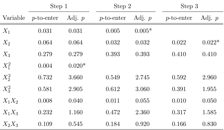
Example for No Hierarchy. Suppose there are three predictor variables, X1, X2, X3, and we
run forward selection using α1 = 0.05 and α2 = 0.01. Thus c = α1/α2 = 5. Table 1 contains
the p-to-enter values and adjusted p-to-enter values for adding any one of the nine total effects into the model for the first three steps of forward selection. Because X12 has the smallest adjusted p-to-enter value at Step 1, 0.020, and this value is less than 0.05, X12 enters. The second part of Table 1 contains the p-to-enter values and adjusted p-to-enter values for adding any one of the eight remaining effects. X1 has the smallest adjusted p-to-enter value, 0.005. Because this value
Table 1: Example of Forward Sequence Using AdjustedP-to-enter Values
Step 1 Step 2 Step 3
Variable p-to-enter Adj. p p-to-enter Adj. p p-to-enter Adj. p X1 0.031 0.031 0.005 0.005*
X2 0.064 0.064 0.032 0.032 0.022 0.022*
X3 0.279 0.279 0.393 0.393 0.410 0.410
X12 0.004 0.020* X2
2 0.732 3.660 0.549 2.745 0.592 2.960
X32 0.581 2.905 0.612 3.060 0.391 1.955 X1X2 0.008 0.040 0.011 0.055 0.010 0.050
X1X3 0.232 1.160 0.472 2.360 0.317 1.585
X2X3 0.109 0.545 0.184 0.920 0.166 0.830
* Indicates the smallest adjustedp-to-enter at each step.
p-to-enter values for adding any one of the seven remaining effects into the model. NowX2 has the
smallest adjusted p-to-enter value, 0.022, and enters the model. Assuming that no more terms are added, the final model usingα1 = 0.05 andα2 = 0.01 contains an intercept, X1,X12, and X2.
3.2 Controlling Two False Selection Rates
In this section the goal is to chooseα1andα2so that the contribution to the false selection rate from
first-order effects (FSRm) is equal to the contribution to the false selection rate from second-order
effects (FSRq), in other words,
E[FSRm] = E[FSRq] =γ0/2. (8)
In order to get a forward sequence of effects using Algorithm 1, the multiplicative factorcof (7) is required. Assuming that there are Nm uninformative main effects and Nq uninformative
second-order effects in the candidate set, Algorithm 1 with fixed α1 and α2 leads to Nmα1 and Nqα2
as approximately the expected number of falsely selected main effects and second-order effects, respectively. SettingNmα1 =Nmα2 and substitutingα1=cα2 (as specified by Algorithm 1) gives
c=Nq/Nm. Therefore,cshould be the ratio of uninformative second-order effects to uninformative
to the target value ofc to be used in Algorithm 1 to achieve (8),
c= 1 +Nq 1 +Nm
. (9)
We now present a method for estimatingc in the No Hierarchy case and then explain how it is used with Weak Hierarchy.
3.3 Fast FSR Sequential Adjustment for No Hierarchy
When estimating bγF(α) for a given α, we assume all effects in the model are informative and all
effects in the candidate set are uninformative. Therefore, with only an intercept in the model there arepuninformative main effects andkT−puninformative second-order effects. Using these values,
the initial estimate forc is
c(1)= 1 +kT −p
1 +p . (10)
Now use the first step of Algorithm 1 with c(1) to obtain a variable X(1) that has the smallest
adjusted p-to-enter value. To update c for the next step, assume that X(1) is an informative variable. Thus, ifX(1)is a main effect, thenc(2) = (1 +kT−p)/p. Alternatively, ifX(1) is a
second-order effect, then c(2) = (k
T −p)/(1 +p). After updating c, we run another step of Algorithm 1
to get X(2) and the adjusted p-to-enter value. To describe the ith step, we need to use the dual
step notation mentioned at the end of Section 2.1: Sm(i−1) andSq(i−1) are the number of main
effect and second-order effects in the model after i−1 steps; Nbm(i−1) = p−Sm(i−1) is the
estimated number of uninformative afteri−1 steps and similarlyNbq(i−1) =kT −p−Sq(i−1) is
the estimated number of uninformative second-order effects. Then at Step iof Algorithm 1,
c(i)= 1 +Nbq(i−1) 1 +Nbm(i−1)
. (11)
After running forward selection as described, we have a sequence of estimates for c, effects entered, adjusted p-to-enter values, and monotonized adjusted p-to-enter values ep1, . . . ,pekT. To define bγF(α), we define Sm(α) =Sm(iα),Sq(α) =Sq(iα), and c(α) =c(iα) at α =pei and constant
elsewhere, whereiα is the largestiassociated with allpei equal toα. Because this is a No Hierarchy
case,Nbm(α) =p−Sm(α) and Nbq(α) =kT −p−Ss(α). Then
b
γF(α) =
b
Nm(α)α+Nbq(α)α/c(α)
1 +Sm(α) +Sq(α)
After calculatingγbF(α) for each pei, we choose the model of size
k(γ0) = max
(
i:pei ≤
γ0[1 +Sm(pei) +Sq(pei)]
b
Nm(pei) +Nbq(pei)/c(pei)
and epi≤αmax
)
, (13)
and letαb1 = supα≤αmax{α:bγF(α)≤γ0}.
3.4 Fast FSR Sequential Adjustment for Weak Hierarchy
In the Sequential Adjustment Method,cchanges at each step of the forward selection process, and under Weak Hierarchy, the candidate set is dynamic, often changing by more than one term at each step. Here we explain how to combine these two approaches.
Under the Weak Hierarchy principle, only thep main effects are initially in the candidate set. With an intercept in the model, we calculate thep-to-enter values for the main effects and select the variable, X(1), with the smallestp-to-enter value. We then update the candidate set by adding the p second-order terms that involveX(1) (p−1 interactions and X(1)2 ). For Step 2, we calculate the p-to-enter values, adjust the p-values for the second-order terms using c(2) = (1 +p)/p, and select
the term, X(2), with the smallest adjusted p-to-enter value. If X(2) is a main effect, then we add thepsecond-order terms that involve X(2) to the candidate set. However, ifX(2) is a second-order effect, then no additional variables are added to the candidate set. In general, for Stepiwe update c using (11), whereNbq(i−1) and Nbm(i−1) are the number of second-order and first-order terms
in the candidate set, respectively, at the beginning of theith step, that is, computed after entering
the (i−1)th variable. The rest of the method is similar to (12) and (13) of the the previous section except that the definitions of Nbm(α) andNbq(α) follow the general prescription from Section 2.2.
4
Simulation Studies
4.1 Simulation for Prediction and Interpretation
We compare the Fast FSR methods with the Least Absolute Shrinkage and Selection Operator (LASSO) (Tibshirani, 1996) and with Bayesian Additive Regression Trees (BART) (Chipman et al., 2006). Recall that all predictor variables are first centered by subtracting the mean and then are divided by the sample standard deviation. Forward selection with p-values determined from the usual least squares F-tests are used in all the Fast FSR methods. Terms above second-order are not considered. The following Fast FSR methods are studied.
Fast FSR with No Hierarchy (FFSR-NH):All kT = 2p+ p2
terms are available at all steps, and model size is chosen by (4).
Fast FSR with Strong Hierarchy (FFSR-SH):InteractionsXiXj are available only after both
Xi and Xj are in the model, whereasXi2 is available afterXi is in. Model size is chosen by (6).
Fast FSR with Weak Hierarchy (FFSR-WH):Interactions XiXj are available only afterXi
orXj are in the model, whereasXi2 is available afterXi is in. Model size is chosen by (6).
Fast FSR with Sequential Adjustment for No Hierarchy (FFSR-NHadj): Same as FFSR-NH except that the second-order p-to-enter values are multiplied by c(i) of (11) at step i. Model
size is chosen by (13).
Fast FSR with Sequential Adjustment for Weak Hierarchy (FFSR-WHadj): Same as
FFSR-WH except that the second-order p-to-enter values are multiplied by c(i) of (11) at step i.
Model size is chosen by (13).
We studied models withp= 20 original predictors, and so there werepq= 230 total predictors.
The original predictors were generated as either N(10,20) or χ2
10 random variables with both
correlated and uncorrelated cases and sample sizes n= 100 and n = 500. N = 100 independent data sets were generated for each situation. Correlated predictors had the following correlation structure:
Corr(Xi, Xj) =
0.7−0.1(|i−j| −1) if 1≤ |i−j|<8, 0 if 8≤ |i−j|<13, 0.7−0.1(19− |i−j|) if 13≤ |i−j| ≤19.
important fact is that there are 20 pairs of X columns with correlations 0.1 to 0.7, respectively, and 50 pairs of columns with no correlation.
The models are:
1. Y =−100 + 25X1+ 15X13−20X17+X12−3X1X9+ǫ;
2. Y =−3 +X1−X4+ 2X9−1.2X13+ 1.6X17+ǫ;
3. Y = 50 + 15X1−25X9+ 1.2X12−1.6X92+ 3X1X9+ǫ.
For each model, ǫ∼N(0, σ2), where σ was chosen to achieve theoretical R2 values 0.25 and 0.50,
where
theoretical R2 = Var
p
X
j=1
βjXj
, Var
p
X
j=1
βjXj +ǫ
.
The key measure of performance used was average model error (AME),
AME = (nN)−1
N
X
i=1 n
X
j=1
(Ybij −µij)2.
To maintain similar scales, results are given in terms of the ratio of the AME of the true model to the AME of a particular method. We call this measure the AME Ratio and note that methods with a high AME Ratio are preferred. The average false selection rate (AFSR) is defined as the average over the Monte Carlo data sets of the number of uninformative effects selected divided by 1 plus the total number of effects selected. AFSR can be partitioned into contributions from main effects, AFSRm, and second-order effects, AFSRq. The average correct selection rate (ACSR) is defined as
the average proportion of informative effects chosen in the model. Note that the denominator used in calculating ACSR is the number of informative terms in the true model. Together, AFSR and ACSR provide a good picture of a method’s variable selection performance.
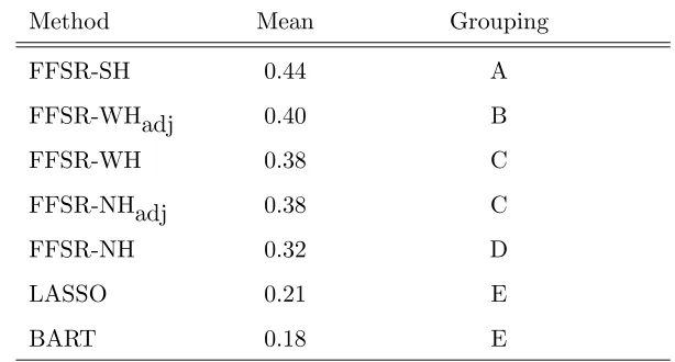
Treating the simulation results as repeated measures ANOVA with 7 methods and a 24 ×3 factorial treatment structure, we fit a linear model in SAS proc mixed with AME Ratio as our response and factors: X distribution (N(10,20) orχ210), predictor correlation (presence or absence), theoretical R2 (0.25 or 0.50), sample size (100 or 500), and model (1-3).
Table 2: Comparison of AME Ratio Means Using Tukey Range Test
Method Mean Grouping
FFSR-SH 0.44 A
FFSR-WHadj 0.40 B
FFSR-WH 0.38 C
FFSR-NHadj 0.38 C
FFSR-NH 0.32 D
LASSO 0.21 E
BART 0.18 E
Methods with the same letter are not significantly different. Standard errors for entries and differences are 0.01−0.02.
methods, No Hierarchy fared the worst, and FFSR-WH and FFSR-NHadj were roughly equivalent, with FFSR-WHadj slightly better than those two. Clearly, p-value adjustment made a major im-provement in the No Hierarchy method and a minor imim-provement in the Weak Hierarchy approach. Overall, BART and the LASSO were not competitive except when n= 100 and R2 = 0.25. The
LASSO generally captured a large proportion of the informative effects, but because it tends to include a large number of effects, it also had large AFSR. Neither the LASSO nor BART used any hierarchy structure, and therefore suffered from overfitting interactions, in addition to lessening interpretability. Yuan, Joseph, and Lin (2007) show how to enforce hierarchy restrictions with LARS, a close relative of the LASSO.
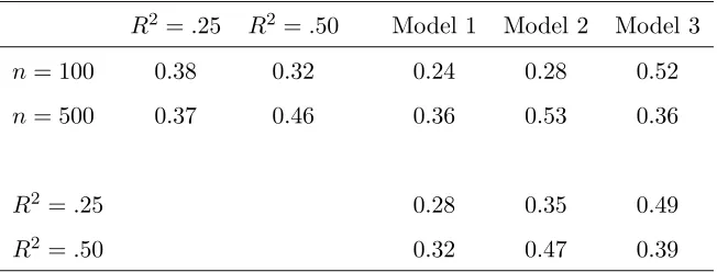
Analysis among only the FSR methods reveals that Method does not interact strongly with the other factors. Among the five factors, model and sample size had large main effects as well as interactions with each other and with sample size. R2 did not have a strong main effect, but it did
have a strong interaction with model. Distribution type for the X matrix (means 0.39 for χ2 and 0.38 for normal) had no significant difference, and correlation within theXmatrix (means 0.40 for no correlation and 0.37 for correlation) had only small effects. Table 3 shows the means for the important effects.
Table 3: AME Ratio Means for Assessing Factor Interactions R2 =.25 R2=.50 Model 1 Model 2 Model 3 n= 100 0.38 0.32 0.24 0.28 0.52 n= 500 0.37 0.46 0.36 0.53 0.36
R2 =.25 0.28 0.35 0.49
R2 =.50 0.32 0.47 0.39
Standard errors of entries are at most .02.
Models 1 and 2, as the sample size andR2 increased, the methods performed better relative to the
true model. However, for Model 3 this was not the case.
For uncorrelated predictors, the Fast FSR methods performed as expected choosing models whose average false selection rates (AFSR) were close to γ0 = 0.05 (not displayed). For correlated
predictors andn= 100, however, AFSR rates were on average around .10 although they generally improved for n= 500. The adjusted Fast FSR methods were designed to ensure that E(FSRm) =
E(FSRq) ≈ E(FSR)/2. The simulation showed that if the original p ×1 vector of predictors
were uncorrelated, then AFSRm and AFSRq were approximately equal when using the adjustment
methods. However, when the predictors were correlated, the AFSR contributions from the two groups were often unequal. For example, at n= 100, R2 = 0.25, and Model 2, FFSR-NHadj had AFSRm = 0.104 and AFSRq = 0.012. For n = 500, those rates improved to 0.035 and 0.018,
respectively.
4.2 Simulation for Response Optimization
For the response optimization study, two response surface designs were used to generate data. The first design was a 73-run, small composite, design with p = 10 factors, where main effects are orthogonal but interactions are correlated with main effects and/or other interactions. The second design was a 100-run, orthogonal, central composite, design with p = 8 factors, where all kT =pq= (2)(8) + 28 = 44 variables are orthogonal.
defined as follows.
1a:Y = 15−3X1+ 1.5X12+ 3X1X9+X2−2X3+ 1.5X4+X5−2X6+X7+X8−X9−5X92+ǫ
1b:Y = 15−5X1+ 1.5X12+ 3X1X9+X2−2X3+ 1.5X4+X5−2X6+X7+X8−7X9−5X92+ǫ
2a:Y = 20 + 2X1−4X12+ 5X1X2+ 3X1X3−3X2−3X22+ 1.5X2X4+ 2X3+ 4X32
− 3X4−2X42+ 2X4X5+ 2.5X5+ 2X6+ 1.5X7+ǫ
2b:Y = 20 + 5X1−3.5X12−X1X2+ 3X1X3−3X2−3X22+ 1.5X2X4+ 2X3+X32
− 4X4−2X42+ 2X4X5+ 3.5X5+ 2X6+ 1.5X7+ǫ.
For each model, ǫ ∼N(0, σ2), where σ was chosen to achieve theoretical R2 values .050, 0.75, or 0.90. As in the first study,N = 100 independent data sets were generated from each model.
Because we are mimicking the situation where screening is conducted prior to the response surface design, we created models with most main effects present. In all the models, only one variable has no effect on the response (X10 in Models 1a and 1b, X8 in Models 2a and 2b). For
Model 1a, the variable X9 has a small main effect but a large interaction with X1 and a large
quadratic effect. The purpose of this model is to illustrate the lack of power of the hierarchy-based approaches to select second-order effects when their parent main effects are small. In Model 1b, the main effects of X1 and X9 are larger. Therefore, we expect the hierarchy methods to perform
better. For Model 2a, the variableX1 has a small main effect but a large interaction with X3 and
a large quadratic effect. As for Model 1a, the hierarchy-based approaches are at a disadvantage for Model 2a becauseX1 must first enter before the large second-order effects have a chance to enter.
In Model 2b, the effects ofX1,X4, and X5 are larger to give the hierarchy methods an advantage.
The goal of response surface modeling is usually to estimate the levels of a process that yield an optimal response. After fitting by Fast FSR, LASSO, or a standard approach where a full model was fit and terms removed if not significant at the α= 0.05 level, each fitted model was optimized to get a set of optimal factor levels. The optimization was carried out subject to the constraint that eachX lies in (−2,2); we call this constrained factor space the region of interest.
and 1b, only variable X9 has an optimal level in the interior the region. For Models 2a and 2b,
variables X1,X2, and X4 all have optimal levels in the interior of the region.
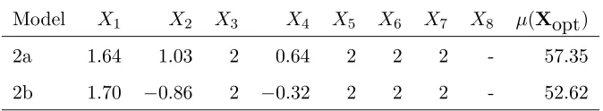
Table 4: Optimal Levels for 10-Factor Small Composite Design Model X1 X2 X3 X4 X5 X6 X7 X8 X9 X10 µ(Xopt)
1a −2 2 −2 2 2 −2 2 2 −0.7 - 48.45 1b −2 2 −2 2 2 −2 2 2 −1.3 - 58.45
Table 5: Optimal Levels for Central 8-Factor Composite Design Model X1 X2 X3 X4 X5 X6 X7 X8 µ(Xopt)
2a 1.64 1.03 2 0.64 2 2 2 - 57.35 2b 1.70 −0.86 2 −0.32 2 2 2 - 52.62
To compare the methods we need a measure of how well a method identifies the optimum levels. The true mean optimal response is µ(Xopt), and the true mean response usingXbopt isµ(Xbopt).
For any factor not selected we set the optimal level at the center point, 0. We refer toµ(cXopt) as the actual performance, whereasµ(Xopt) is the optimal performance. The standardized difference,
{µ(cXopt)−µ(Xopt)}/µ(Xopt), is a measure of how close a method performs relative to the true optimal performance. When analyzing a real data set, the estimate of the optimal response is b
µ(cXopt), but that is not used in this simulation.
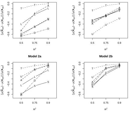
Figure 1 illustrates the mean performance for each method. Because Fast FSR with Sequential Adjustment for Weak Hierarchy (FFSR-WHadj) was always better than Fast FSR with Weak Hierarchy (FFSR-WH), and Fast FSR with Sequential Adjustment for No Hierarchy (FFSR-NHadj) was always better than Fast FSR with No Hierarchy (FFSR-NH), FFSR-WH and FFSR-NH were left off the figure. For Model 1a, Fast FSR with Strong Hierarchy (FFSR-SH) and FFSR-WHadj performed poorly. The reason is that X92 andX1X9 are both large effects, but the main effect X9
is relatively small, thus making it hard for these second-order terms to enter. The LASSO and FFSR-NHadj performed the best in Model 1a, with the LASSO better for R2 = 0.5 and FFSR-NHadj better for R2 = 0.9. For Model 1b, the methods performed fairly equally with FFSR-SH,
FFSR-NHadj, and LASSO among the best. The LASSO does best with smaller R2, and FFSR-NHadj is better for larger R2
L L L −0.6 −0.4 −0.2 0.0 R2 { µ ( X ^ o p t ) − µ ( Xo p t )} µ ( Xo p t ) Model 1a
0.5 0.75 0.9
U U U A A A D D D S S S T T T L L L −0.6 −0.4 −0.2 0.0 R2 { µ ( X ^ o p t ) − µ ( Xo p t )} µ ( Xo p t ) Model 1b
0.5 0.75 0.9
U U U A A A D D D S S S T T T L L L −0.6 −0.4 −0.2 0.0 R2 { µ ( X ^ o p t ) − µ ( Xo p t )} µ ( Xo p t ) Model 2a
0.5 0.75 0.9
U U U A A A D D D S S S T T T L L L −0.6 −0.4 −0.2 0.0 R2 { µ ( X ^ o p t ) − µ ( Xo p t )} µ ( Xo p t ) Model 2b
0.5 0.75 0.9
U U U A A A D D D S S S T T T
Figure 1: Scaled average difference in actual and optimal performance. Values close to zero are better. True Model (T), Standard Approach (U), LASSO (L), FFSR-SH (S), FFSR-NHadj (A), and FFSR-WHadj (D). The standard errors of all plotted points are bounded by 0.03.
this model, X12 is very important, but its main effect is relatively small. Therefore, FFSR-NHadj performed best. For Model 2b, FFSR-NHadj again performed the best overall.
general, when R2 = 0.5, the bagged Fast FSR methods were superior to their regular versions in estimating the optimal factor levels. However, as R2 increased to 0.9, bagging yielded little or no improvement. The only exception was for the hierarchy-based approaches on Models 1a and 2a. In these models, bagging overcomes the problems of fitting large second-order terms with weak parent main effects.
A standard approach is to fit the full response surface and eliminate terms not significant at the α= 0.05 level. This approach performed poorly for Models 1a and 1b, but performed very well for Models 2a and 2b. Possible reasons for the poor performance in Models 1a and 1b are the sparsity of the true models, the large number of factors, and the correlation between interactions in the design matrix. Even when the standard approach performed well, it still had large false selection rates. Therefore, we recommend FFSR-NHadj, especially in studies with a large number of factors; or a bagged version of FFSR-SH. From this study, it is clear that the power of a method to select informative quadratic and interaction terms is important when optimizing a response.
5
Examples
Example 1. Response Optimization in the Cutinase Study. Cutinase is an enzyme excreted by fungi that is used in many industrial products and processes, including laundry and dish washing detergents. Many current procedures to produce cutinase are time-consuming, expensive, and have low yield. Pio and Macedo (2008) used response surface modeling to study the key factors for maximizing cutinase production. Table 6 describes the variables in their study.
In order to produce cutinase, a medium of potato dextrose agar was prepared with nutri-ents added before cultivation. Pio and Macedo were interested in determining the optimal con-centration levels of the following nutrients: flaxseed oil; K2HPO4; MgSO4; NaNO3; KCl; and
FeSO4·7H2O. Using a 20-run fractional factorial design for screening, only flaxseed oil, NaNO3,
KCl, and FeSO4·7H2O were significant factors. Nevertheless, Pio and Macedo proceeded with an
Table 6: Variables in Cutinase Study Variable Name Measurement Units X1 flaxseed oil %
X2 K2HPO4 %
X3 MgSO4 %
X4 NaNO3 %
X5 KCl %
X6 FeSO4·7H2O %
Y cutinase units/mL (U/mL)
We used Fast FSR methods withγ0= 0.05 to analyze the data, and all methods gave the same
model listed in Table 7. All six nutrients were identified as important for maximizing cutinase production. K2HPO4, MgSO4, and NaNO3 all interacted positively with FeSO4·7H2O. Similarly,
K2HPO4 and MgSO4 interacted positively with NaNO3. The only nutrients that did not appear to
interact with each other were MgSO4 and KCl. The standard approach of fitting the full response
surface and eliminating terms not significant at the 0.05 level gave the same model except forX2X4.
Table 7: Model Summaries for Cutinase Production
Method Effects in Model R2 AdjustedR2
Pio and Macedo X1,X12,X2,X22,X3,X32,X4,X42, 0.55 0.47
X5,X52,X6,X62
Fast FSR Methods X1,X12,X2,X22,X3,X32,X4,X42, 0.78 0.72
X5,X52,X6,X62, X2X4,X2X6,
X3X4, X3X5,X3X6,X4X6
Standard Approach X1,X12,X2,X22,X3,X32,X4,X42, 0.77 0.71
X5,X52,X6,X62, X2X6,
X3X4, X3X5,X3X6,X4X6
Table 8: Optimal Levels and Maximum Cutinase Production
Method X1 X2 X3 X4 X5 X6 µ(b Xbopt) Pio and Macedo −0.42 −0.38 −0.38 −1 −0.32 −0.59 12.33 Fast FSR Methods −0.42 −1 −1 −1 −0.14 −1 15.56 Standard Approach −0.42 −0.80 −1 −1 −0.15 −1 15.11
maximumµ(b Xcopt) = 12.33 U/mL (somewhat greater than their 11.09 U/mL for all factors set to the lowest levels). Optimizing the 18-variable model in Table 7 chosen by the Fast FSR methods results in the estimated maximum µ(b cXopt) = 15.56 U/mL. Maximizing the model obtained by the standard approach yields the estimated maximum µ(b cXopt) = 15.11 U/mL. Table 8 gives the coded optimal factor levels and estimated maximum for these three models. These results suggest that Pio and Macedo’s response optimization underestimates maximum cutinase production.
Example 2. Dual Response Optimization in the Lipase Study. Lipase is an enzyme used in industrial and food processes for its ability to break down lipids. Rathi et al. (2002) used response surface modeling to maximize both the production of lipase and its ability to break down fatty acids or specific activity. In order to produce lipase, the bacteria Burkholderia cepacia was cultivated with concentrations of glucose and palm oil added as nutrients. In addition to the nutrient factors, Rathi et al. (2002) were interested in the effect of incubation time, inoculum density, and agitation on the two response variables. Table 9 lists the variables in their study.
Table 9: Variables in Lipase Study Variable Name Measurement Units
X1 glucose mg/mL
X2 palm oil % by volume (% v/v)
X3 incubation time hours
X4 inoculum density %
X5 agitation rev/min
Y1 lipase units/mL (U/mL)
Y2 specific activity units/mg (U/mg)
Table 10: Model Summaries for Lipase Production
Method Effects in Model R2 AdjustedR2
Rathi et al. X1,X12,X2,X22,X3,X32,X4,X42,X5,X52 0.74 0.62
FFSR-SH No effects 0.00 0.00
FFSR-WH No effects 0.00 0.00
FFSR-WHadj No effects 0.00 0.00
FFSR-NH X22 0.26 0.24
FFSR-NHadj X2
2,X3,X42 0.53 0.48
Standard Approach X2,X22,X3,X4,X42 0.58 0.50
linear model in all five factors excluding their interactions. Using their models, the estimated maximum lipase production is 31 U/mL and maximum activity is 110 units/mg.
We used Fast FSR methods withγ0= 0.05 to analyze the data. The selected variables for each
method and response are listed in Tables 10 and 11. Unlike the cutinase example, the Fast FSR methods did not choose the same effects in their final models. FFSR-SH and FFSR-WH appear to underfit the data. Because the main effects were not selected, these approaches were unable to fit the significant quadratic terms. Conversely, FFSR-NHadj fit larger, more reasonable models. For lipase production no effects were common to all models, although it is likely that palm oil, incubation time, and inoculum density all influence lipase production in some manner. For specific activity only incubation time is common to all the models, whereas glucose was the only factor not selected by any Fast FSR method.
The standard approach models in Tables 10 and 11 show which variables had Type IIIp-values less than 0.05. Thus, of the full ten-variable model used by Rathi et al. (2002), only X22, X3,
X42, and X52 are statistically significant at 0.05 level for both responses. Additional simulations in Crews (2008) suggest that their ten-variable models are possibly too large.
Following Rathi et al. (2002), we maximized lipase production and specific activity subject to
−1 ≤ Xj ≤ 1. Tables 12 and 13 give the coded optimal factor levels and estimated maximum
Table 11: Model Summaries for Specific Activity
Method Effects in Model R2 AdjustedR2
Rathi et al. X1,X12,X2,X22,X3,X32,X4,X42,X5,X52 0.81 0.71
FFSR-SH X3 0.17 0.14
FFSR-WH X3 0.17 0.14
FFSR-WHadj X3 0.17 0.14
FFSR-NH X2,X22,X3,X42,X52 0.75 0.71
FFSR-NHadj X2,X22,X3 0.57 0.52
Standard Approach X2,X22,X3,X4,X42,X5,X52 0.78 0.71
inoculum density,X42, is not chosen in the model for lipase activity. Without this term the model estimates maximum activity to be approximately 73 U/mg, whereas including this term increases the estimate to approximately 90 U/mg. Further investigation shows that the next possible model in the forward sequence, which addsX2
4 andX52, has bγF just over the 0.05 limit. Using this model
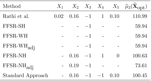
for maximization leads to 100.63 U/mg. Based on these results, the optimal factor levels for glucose, palm oil and agitation are close to the center point. The optimal factor level for incubation time is the low level, and the optimal level for inoculum density is the high level. Using these optimal levels, the estimated maximum lipase production is approximately 23 U/mL, and the estimated maximum activity is approximately 90−100 U/mg. Therefore, it is likely that the maximum lipase production and specific activity observed in practice would be smaller than the estimates 31 U/mL and 110 units/mg. provided by Rathi et al.
Table 12: Optimal Levels for Maximum Lipase Production Method X1 X2 X3 X4 X5 µb1(Xbopt) Rathi et al. 0.01 0.09 −1 1 0.09 31.11
FFSR-SH - - - 10.01
FFSR-WH - - - 10.01
FFSR-WHadj - - - 10.01
FFSR-NH - 0 - - - 13.67
FFSR-NHadj - 0 −1 1 - 22.98
Table 13: Optimal Levels for Maximum Specific Activity Method X1 X2 X3 X4 X5 µb2(Xbopt) Rathi et al. 0.02 0.16 −1 1 0.10 110.99
FFSR-SH - - −1 - - 59.94
FFSR-WH - - −1 - - 59.94
FFSR-WHadj - - −1 - - 59.94
FFSR-NH - 0.16 −1 1 0 100.63
FFSR-NHadj - 0.19 −1 - - 73.61 Standard Approach - 0.16 −1 −1 0.10 100.45
6
Conclusion
Fast FSR methods provide a simple approach to analyzing response surface experiments as well as for many other applications where quadratic terms are of interest. Although the Strong Hierarchy restriction (FFSR-SH) has intuitive appeal and performed best in our first simulation study that had p = 20 original variables, it can perform poorly in models where there are important second-order effects but weak parent main effects. In particular it did not perform very well in our second simulation study involving response optimization. Using no hierarchy restrictions (FFSR-NH) can prevent strong second-order effects from being missed. However, second-order terms often dominate the forward sequence, so adjusting the p-values with FFSR-NHadj is recommended. In general, bagging both FFSR-SH and FFSR-NHadj show improvement when estimating optimal factor levels.
ACKNOWLEDGEMENTS
This work was supported by NSF grant DMS-0504283. SAS macros for computing Fast FSR variable selection are available athttp://www4.stat.ncsu.edu/~boos/var.select.
REFERENCES
Breiman, L. (1996), “Bagging Predictors,”Machine Learning, 24, 123-140.
Chipman, H. A., George, E. I., and McCulloch, R. E. (2006), “BART: Bayesian Additive Regression Trees,” preprint.
Crews, H. B. (2008), “Fast FSR Methods for Second-Order Linear Regression Models,” unpublished Ph.D. dissertation, North Carolina State University, Dept. of Statistics.
Pio, T. F., and Macedo, G. A. (2008), “Cutinase Production by Fusarium oxysporum in liquid medium using central composite design. Journal of Industrial Microbiology and Biotechnology, 93, 930-936.
Rathi, P., Goswami, V. K., Sahai, V., and Gupta, R. (2002), “Statistical Medium Optimization and Production of a Hyperthermostable Lipase fromBurkholderia cepaciain a Bioreactor. Journal of Applied Microbiology, 35, 59-67.
Tibshirani, R. J. (1996), “Regression Shrinkage and Selection via the LASSO,”Journal of the Royal Statistic Society, Series B, 58, 267-288.
Wu, Y., Boos, D. D., and Stefanski, L. A. (2007), “Controlling Variable Selection by the Addition of Pseudovariables,” Journal of the American Statistical Association, 102, 235-243.