Optimal control of a queueing system with three heterogeneous servers

OPTIMAL CONTROL OF A QUEUEING SYSTEM

WITH THREE HETEROGENEOUS SERVERS

Ioannis Viniotis

Center for Communications

&

Signal Processing Department of Electrical and Computer Engineering

North Carolina State University Raleigh, NC 27695-7914

CCSP-TR-89/5

Abstract

We study the problem of optimally controlling a three server queueing system. Ar-riving customers join a single queue, which is served by three servers, 8₁,52 and 53. The

servers are exponential, but of different rates. The total expected time a customer spends in the system is to be minimized. We show that the optimal policy can be characterized

by three thresholds, m3,mb and mi, such that: 51, the fastest server, should be always busy; 53, the slowest server, should be activated only when m3 or more customers wait in

the queue, and, given that 53 is idle (busy), 82 should be activated only when mi (mb)

customers wait in the queue. We use stochastic dominance arguments to establish the results.

1. Introduction

We consider the queueing system shown in figure 1. Customers arrive at an (infi-nite capacity) buffer in a Poisson stream of rate ~. The buffer is served by three servers

51' 52, 53, of different capacities PI, P2 and pj respectively. Without loss of generality, we assume that ILl

>

1L2

>

1L3

>

o.

The service requirements are exponentially distributed, with parameter 1. Thus the time a customer spends at server 5i is exponentially dis-tributed, with parameter Pi. To avoid trivial cases, we assume that 0

<

_~

<

PI

+

1-£2

+

1-£3.

----.~ III~

.1-.

The motivation for studying this model comes from applications in dynamic routing in computer networks and communication systems. The more general system with N servers would be a more appropriate model of real life applications; however, the enormity of the problem forces us to follow a moderate step-by-step approach.

studied in

[1].

In

[1],

Lin and Kumar have shown that the optimal policy (i.e., the one that

minimizes the mean sojourn time of customers in the system), is of threshold type. In other

words, the optimal policy keeps the faster server busy, whenever possible, and activates

the slower server only when the number of waiting customers exceeds a certain threshold.

Moreover, they have provided a simple formula to calculate the optimal threshold, as a

function of the statistical parameters of the model. In

[2],

Agrawala et al considered a

related problem, with an arbitrary number, N, of servers, but no arrivals. They have

shown that a threshold type policy minimizes the expected total flow time (sum of all

finishing times). They also provide a simple formula to calculate the threshold for each

server. In [4,7,8,9] other scheduling problems with N servers have been considered.

Our goal is to minimize the expected time a customer spends in the system, by properly

selecting the customer allocation strategy. Whenever one or more servers become idle,

and there are customers waiting for service, one mayor may not decide to forward one

or more customers for service. We show in this paper that the optimal policy (among

all nonanticipative, nonpreemptive policies) is of threshold type (to be precisely defined

later), i.e., it may idle a server, even when there are waiting customers. We used stochastic

dominance arguments to establish this result, as was done in

[3]

for the

MtMt2

case. We

were not able to utilize Dynamic Programming arguments.

The paper is organized as follows. In section 2 we describe the queueing model of the system and inroduce some notation. In section 3 we present the results; the proofs

are provided in the appendix. Since the technique we are using is based on the arguments

presented in [3], we omit lengthy details, whenever they can be readily found there. Where

necessary, we emphasize the basic differences and provide only a sketch of the proof.

We conclude with a conjecture regarding the MIMIN model and some implementation

remarks.

2. The model

The system consists of a single queue, served by three unequal speed servers. Arrivals

are Poisson of rate

A.

The service discipline is nonpreemptive*; service time at server

Si

is

gen-exponential, with rate lLi· To ensure stability of the system, we assume that A

<

ILl

+

1L2

+

1L3' As mentioned above, we may assume without loss of generality that ILl

>

1£2

>

1£3'

Let

ZOt denote the number of customers waiting in queue, at time

t.

Zit denote the busy-idle condition of server S· ,; -_{" c, -} 1 2 3_{, , •}

If Zit

=

0 (1), we say that the server is idle (busy).

Under the statistical assumptions we adopted, the vector

is a suitable state description of the system. The state space of the system is

X~{O,l,

...} x {O,1}3

A policy l'is any (nonanticipative, nonpreemptive) rule which at every time t decides

(on the basis of the history

{x.,

8 ::;

t}),

whether to activate one or more idle servers, given

that the queue is nonempty. We shall refer to allocation decisions as actions of the policy.

Let 1:1;tI~:l;Ot

+

:l;1t

+

:l;2t

+

:l;3t denote the total number of customers in the system

(queue and servers) at time

t.

For a given discount factor 0:

>

0, we define the expected,

a-discounted cost incurred by policy" when starting from initial state xo

=

z , at time

t

= 0, as

(1)

Here E~ denotes expectation with respect to the probability law of the process Xt, when

the policy, is used and the initial state is z , We are primarily interested in the average

cost criterion; however, in view of the results in [5], it suffices to consider the discounted

cost criterion only.

eral MI1\JIN case): keep all servers busy and preempt the slowest (currently busy) server

whenever a faster server becomes idle; reallocate the preempted customer to the recently

available server. In computer systems preemptions may be allowed; however, in

A policy is optimal if it minimizes the cost given in equation (1). It is known that

the optimal policy for this problem is Markov, deterministic and stationary [5]. Let 1r be

the optimal policy. It can be described as follows. Whenever a transition (an arrival or

a service completion) occurs, that brings the system to state y, 1r chooses an action that

makes the state jump to the value

To simplify the notation, we shall use

i==1,2,3

to denote the actions of the optimal policy. For example, 1r(YO,Y1,Y2,Y3)3

==

1 (0) means

that at state (Yo,Yl,Y2, Y3) the optimal policy decides to activate the slowest server (keep it idle).

Remark: When the optimal policy assigns customers to more than one idle servers

simultaneously, we will assume, without loss of generality, that it does so in a sequential

manner, from the fastest to the slowest server.

3. Characterization of the optimal policy.

Our objective in this section is to characterize the structure of the optimal policy, 'Jr.

We shall make use of the following definition.

Definition: A policy / is called a threshold type policy (with thresholds m3,mb,mi) if:

• it keeps 81 , the fastest server, busy whenever possible, i.e., whenever the queue is

nonempty.

• it allocates a customer from the queue to the slowest server, 53, iff at least m3

cus-tomers wait in the queue, and

• it activates server 82 when at least m.; (mb) customers wait in the queue and server

83 is idle (busy).

Remark: The fact that a threshold policy will activate a server only when the queue

size exceeds the corresponding threshold does not mean that the server can not be busy

We wish to show the following theorem.

Theorem: The optimal policy for the cost criterion (1) is a threshold type policy.

The proof is is based on lemmata 1-6 below, which describe certain of the

proper-ties of the optimal policy. The following proposition, our main result, is an immediate

consequence of the ergodicity assumption and the results in [5].

Proposition: The policy that minimizes the expected time a customer spends in the

system is of threshold type.

The following lemmata describe the properties of the optimal policy for the discounted

cost criterion. They are self-explanatory. Their proofs are presented in the appendix.

Lemma 1: The optimal policy should activate a faster rather than a slower server.

Lemma 2: The optimal policy should keep the fastest server busy whenever customers

wait in queue.

An immediate consequence of lemma 2 is that for states (ZO,ZI,Z2,Z3) with Zo

2:

1,

we should have Xl

=

1, since states

(xo,

0,X2,Z3) will occur only instantaneously (i.e., just

before 1r takes an action).

Lemma 3 (4) characterizes the actions of the optimal policy for the second server,

when the system visits states in which the slowest server is idle (busy).

Lemma 3: Given that 53 is idle, the optimal policy should activate the second server,

52, only when at least tti; customers wait in the queue.

Lemma 4: Given that 53 is busy, the optimal policy should activate 52, only when

at least fib customers wait in the queue.

From the remark of the previous section and lemma 1 we see that 1r should consider

activating 8₃ only in states

(Yo,

1, 1,0). The next lemma characterizes these actions.

Lemma 5: The optimal policy should activate the slowest server only when at least

m3 customers wait in the queue.

A complete characterization of the optimal policy would require computation of the

three thresholds, as a function of the statistical parameters of the model. We have only

Lemma 6: mi

<

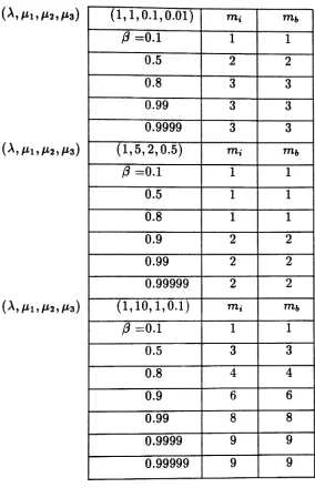
m3,mb ~ m3·

We have not been able to provide a relationship between mi and mb· However, we

strongly suspect that mi == ms: In this case, the optimal policy for activating the second

server will be a pure threshold policy, with a threshold that depends on the queue size

only, and not the condition of the third server. This conjecture is in compliance with the

results in [2]. Moreover, it is backed up by extensive numerical calculations of the optimal

policy, using value iteration on the Dynamic Programming Equation.

4. Conclusions

We have studied the structure of the optimal policy for a three server queueing

sys-tem. We have shown that the optimal policy is of threshold type, with the threshold for

the second server possibly depending on the busy /idle condition of the slowest server.

Stochastic dominance arguments were used to obtain the result. They strongly rely on

the number of servers; their extension to the more general case of N

>

3 servers is not

straightforward. It is possible, however, to obtain the structure for this case as well, using

Linear Programming based arguments, as described for example in [6].

The proof presented here is not constructive; therefore it does not suggest how the

optimal policy thresholds can be computed, for the implementation of the optimal policy.

The straightforward method of calculating the cost as a function of the thresholds

[1]

cannot be applied here. We suggest to use the value iteration for the discounted cost as a

reasonable heuristic. In all cases we tried, it converged quite rapidly. Figure 2 shows the

behavior of the optimal thresholds as a function of the discount factor, for given arrival

and service rates. It also "supports" the previously mentioned conjecture, mi == mb.

Appendix

In this appendix we provide the proofs of lemmata 1-6. Throughout this appendix,

Ui will denote an exponential random variable with rate J-Li. It represents the service time

of a typical customer, at server Si. Whenever the proofs are similar, the reader is refered

to [3] for the missing details. The basic idea is to construct a nonstationary, nonMarkov

policy, 1r,which will improve the optimal policy 11",whenever the latter does not have the

Proof of lemma 1: Assume that i

<

j and let O"i,O"; be the service times of a given

customer, when it is served by server Si or Sj respectively. By stochastic dominance, we

may assume that O"i

<

(Tj.

Consider two initial states, s, and 8;, such that at state 8i (8;) server 8i (8;) is active

and server

S; (Si)

idle. The remaining state components are the same. Let T be the first

time that 7r activates server

Si

when starting from initial state

Si

(T ~ (0). Clearly, if

T

>

CTi,then

J(Si)

<

J(8;).

If T

<

O'i, then

J(Si)

==

J(s;)

and thus the cost when starting from s, is always no more then the cost when starting from 8;.

Note, however, that this does not necessarily mean that it is optimal to activate server

5i

in a state with Yo ~ 1,5i

==

0,5j == 0. Idling both servers may be optimal.

Proof of lemma 2: By lemma 1, whenever server 51 is idle, it should be prefered to

other idle servers. Since idling the fastest server is easily shown to be suboptimal, the

result follows.

Proof of lemma 3: From lemma 1 we know that 71" will not activate server

53

if it does

not activate (at the same state) server 52. From lemma 2, we should only consider states

of the form (Yo,1,0,0). It is easy to show that there exists at least one state with Yo

<

00,

such that

The proof is essentially that of lemma 3.2b in [3], since by hypothesis if 71" does not utilize

server

S2,

it will never utilize server

53

as well; in this case, the system behaves essentially

as an MIMI2 system. Therefore, we will not repeat it here.

Suppose now that for some queue size Yo ,we have that 71"(Yo, 1,0,0)2 == 1 and 71"(Yo

+

1,1,0,0)2

==

o.

Let Tj be the first time that 71" activates server 5j , j

==

2,3, when starting

from an initial state (Yo

+

1,1,0,0). From lemma 1, we have that T2 :::; T3 a.s,

Suppose that another policy ;r activates

52

at t

==

o.

If CT2 :::; T2, then ;r improves

7r. If 0"2

>

T2' then the trajectories under 7r,

*

are matched, since at

t

=

T2 we have

Xt

=

(Yo,

1, 1,0) (or

(Yo -

1,1,1,1)) and thus Xt

=

Xt· Moreover, under 7r, the queue size

never reached 0 in [0,T2], qed.

which the optimal policy utilizes server 52. We then show that 1r activates the server in

state (Yo

+

1,1,0,1) as well.

To show the first part of he claim, choose Yo

>

mi, where mi is defined as in lemma 3 and let the system be at state (Yo, 1, 0, 1) at time

t

=

0. Let 0"3 be the service time of the

customer served by server 53.

By hypothesis, 1r will never activate 52 in

[0,0'3);

let another policy ;r activate 52 when starting from (Yo,1,0,1). Let T be the first time to reach queue size mi from size Yo,

under 1r. Clearly T increases (stochastically) as Yo increases.

For all sample paths with 0"3 :::; T, 11" will activate 52, since a state (Yo, 1, 0,0) will be

reached at t

=

0'3, with Yo

2:

mi. For those sample paths, 7r can only improve 7T". For all

sample paths with 0'3

>

T, 1r does not activate 52, and 7r may incur a higher cost. However,

the probability of those paths can be made arbitrarily small, by increasing Yo.

To show the second part of the claim, we may proceed along the lines of the proof of

lemma 3.2(3) in [3], with minor modifications.

Proof of lemma 5: As in the previous two lemmata, again the proof has two parts,

although now it is more elaborate. We first have to show that 1r will activate 53 at some

state (Yo,l,l,O), with Yo

<

00. We then show that it does so at state (Yo

+

1,1,1,0) as

well.

The proof of the first part of the claim is quite similar to that of lemma 4. Let T

denote the first time to reach an empty queue, under 7r. We may similarly observe that

for sample paths with 0"3 :::; T, activating 53 is better than idling it. As Yo increases, the

probability of those paths increases.

For the second part, observe that since the optimal policy is ergodic (all thresholds

are finite), the state (0, 0, 0, 0) will be eventually visited. From this state we'll visit state

(Yo

+

1,1,0,0), and from lemma 1 we visit state

(Yo,

1, 1,0) before we visit a state with

the slowest server busy. Thus, if at a state (Yo, 1, 1,0) it is optimal to activate 53, at state

(Yo

+

1,1,0,0) it is optimal to activate 82 • With this observation in mind, we may now

proceed as in lemma 3.2(3) of [3].

(1)), when the initial state is z , For any state (Yo,I,O,I) with Yo

<

mb, we have

J(yo -1,1,1,1)

>

J(yo,l,O,l)

since it is better to keep 52 idle. From lemma 1 we have

J(Yo,l,O,l) ~ J(Yo,l,l,O)

and thus

J(yo - 1,1,1,1)

>

J(yo,1,1,0)

which implies that Yo

<

m3. Thus mb

:S

m3.

As already mentioned in the proof of lemma 5, we visi t state (Yo, 1, 1, 0) before we

References

[1] W. Lin-P. R. Kumar, "Optimal Control of a Queueing System with Two Heterogenous

Servers," IEEE Transactions on Automatic Control, vol. AC-29, pp. 696-703, Aug.

1984.

[2] A. Agrawala et aI, "A Stochastic Optimization Algorithm Minimizing Expected Flow

Times on Uniform Processors," IEEE Transactions on Computers, vol. C-33, pp.

351-356, 1984.

[3] J. Walrand, "A Note on Optimal Control of a Queueing System with Two

Heteroge-nous Servers," Systems and Control Letters, Vol. 4, pp. 131-134, 1984.

[4] R. Weber, "On the Optimal Assignment of Customers to Parallel Servers," Journal

Appl. Prob., vol 15, pp. 406-413, 1978.

[5] S. A. Lippman, "Semi-Markov Decision Processes with Unbounded Rewards,"

Man-agement Science, Vol. 19, pp. 717-731, 1973.

[6] I.Viniotis-A. Ephremides, "Optimal Switching of Voice and Data at a Network Node," Proceedings of the 26th CDC, pp. 1504-1507, Los Angeles, CA, December 1987.

[7] E. G. Koffman et al, "Minimizing Expected Makespans on Uniform Processor

Sys-tems," Adv. Applied Prob., 19, pp. 177-201,1987.

[8] P. R. Kumar-J. Walrand, "Individually Optimal Routing in Parallel systems," J.

Applied Probability, vol. 22, pp. 989-995, 1985.

(1, 1,0.1,0.01) mi mb

(3 =0.1 1 1

0.5 2 2

0.8 3 3

0.99 3 3

0.9999 3 3

(1,5,2,0.5) mi mb

(3 =0.1 1 1

0.5 1 1

0.8 1 1

0.9 2 2

0.99 2 2

0.99999 2 2

(1,10,1,0.1) mi mb

{3 ==0.1 1 1

0.5

3 3

0.8 4 4

0.9 6 6

0.99 8 8

0.9999 9 9

0.99999 9 9

Figure 2.