Phenomena of reverse pressure pulse in piping during fast fluid injection
Raj Kumar Singh, Sunil Kumar Sinha and A.Rama Rao*
Vibration Laboratory Section, Reactor Engineering Division, Bhabha Atomic Research Centre, Mumbai-400085, India
Abstract
A study was carried out to investigate hydraulic behavior in a piping loop connected to a high-pressure fluid injection system. An experimental setup was erected with required front-end instrumentation to monitor the parameters during quick fluid injection. The fast injection of fluid from a small tank in to a larger tank was achieved by quick opening of a solenoid valve connected between the tank and a pneumatic system. The time taken for complete injection, the impulsive forces seen by the structures and variation in the fluid pressure at different section of the loop was monitored. It was also observed that, a delayed reverse pressure manifest in the loop after the injection. The possibility of reverse pulse in the pipe has been assessed and estimated by basic fluid dynamic formulation.
Introduction
Pressure pulses are common in hydraulic system used for different purposes in industries. In many of the oil hydraulic system, high-pressure hose are connected to convey the pressurized fluid to the working device. During every injection stroke, the hose deflects due to transmission of pressure pulse in the system. This can be seen in hydraulic power packs connected to large size shake tables used for vibration testing of components. Forward and backward movement of pressure pulse is common in these hose.
Whereas in reciprocating pumps, gas filled accumulators (gas bottles) is connected to the discharge pipe to absorb the pressure pulsations, which are harmful to the systems connected at the down stream of the pipe. The intensity of pressure pulse and its direction of propagation entirely depend on the total system dynamics pressure field.
In one of the developmental project, it was required to study the behavior of the pressure pulse during and after fast injection of fluid from a small tank to a larger tank. An experimental setup was erected which was closely simulating the actual operating condition and structural design [1],[2]. In the setup, it was important to accurately measure the fluid injection time from small tank to large tank. The time of injection was accurately measured by time difference in the vibration signal picked up from the tank during injection. Besides measuring the time taken for complete injection, the impulse force seen by the structures and variation in the fluid pressure at different section of the loop before, during and after the injection was monitored. It was also observed that, a delayed reverse pressure pulse travel from larger tank to smaller tank several seconds after the injection. The possibility of reverse pulse in the piping loop has been assessed and estimated by basic fluid dynamic formulation. The paper gives the detail of measurement of injection time, proof of reverse pulse in the pipe and its timing,
analytical estimation of the reverse pressure pulse using basic fluid dynamic formulations and the velocity profile of injection through a perforated tube installed in the larger tank.
The test setup
Figure 1 shows schematic arrangement of the experimental setup. It consists of a tank holding about 10 litres of water. Figure 2 shows inside of the tank. The water flows out of the tank from 50 mm diameter pipe, which gets connected to a larger tank. The length of the outlet pipe is 3.0 meters. The top of the tank is connected to a gas circuit maintained at a nominal pressure of 60 bars. A rubber ball floats on the water level in the tank whose size is chosen such that it moves freely within the tank when the gas pushes it down. When the injection is activated, the high-pressure gas acts in the tanks thus pushing the ball to the bottom of the tank. In the process, the water gets injected in to the tank. The velocity of the ball in the tank is of the order of 2 m/s. During the transient, there is all possibility of some quantity of water leaking to the upper portion of the ball and to remain in the tank above the ball.
Figure 1 Experimental Test Set up
Inside the larger tank, the injected water jets out from the perforation in the tube installed horizontally as shown in figure 1.
Figure 2. Details of Small Tank
One of the important aims of the experiment was measure the total time of injection of water from the small tank to the larger tank. It was planned to capture the time of impact of the rubber ball at the bottom of the tank and the time of trigger signal to open the gas pressure into the tank. The time difference between the two gives the time of injection. To capture the impact signal, vibration sensor was mounted at the bottom of the tank. After injection, the ball remains seated at the bottom of the tank due to high gas pressure acting on the ball. This prevents escape of gas into the larger tank. The top and bottom of the tank is also instrumented with pressure transducers to record the pressure in the loop at different time during the injection. The pressure tapping points can be seen in figure 2. One pressure transducer measures pressure in the outlet pipe of the tank.
Measurement of Injection time
An accelerometer mounted at the bottom of the tank captures the ball impact signal at the bottom of the tank. This signal precisely gives the time of the ball reaching at the bottom of the tank, which in other words is the time when the water is completed injected. To know the starting time of injection, current signal from one of the solenoid valve that lets gas into the tank was acquired simultaneously. The difference in the arrival of the current signal and the vibration signal due to impact of the ball was precisely measured to arrive at poison injection time from the tank. To the measured time difference, the time required for the complete opening of the solenoid valve and other residual time were added to arrive at total time of injection. The average injection time arrived at after several trials were in the range of 2.35 to 2.45 seconds, which was as per the design requirement.
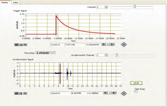
Figure 3 shows snap shot of the current and vibration signal at the instant of water injection. The time difference between the two signals is highlighted.
Figure 3 Snap Shot Showing Current Signal and Vibration Signal
Figure 4 shows the snap shot of the complete signal after the injection. It can be seen in the figure that more than one vibration signal has been captured after the impact of the ball indicating that some secondary impact happen after the ball is seated at the bottom.
Figure 4 Current and Vibration Signal Showing Multiple Impact
Rebound of the ball inside the tank was ruled out as the second and the third vibration signals come after several seconds and besides the gas pressure on the top of the ball does not allow the ball to rebound even once. It has been seen that the gas pressure keeps the ball pressed against the bottom seat of the tank.
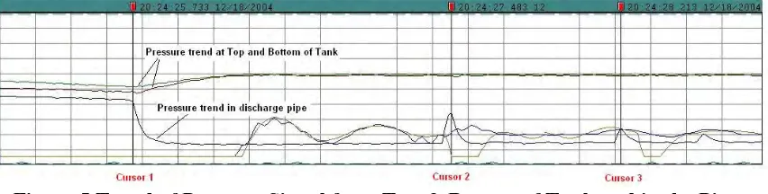
Figure 5 shows the trend of pressure signal measured at top and bottom of the tank and also in the pipe down stream of the tank. The first cursor location in the figure is the time when the rubber ball strikes at the bottom of the tank. Before this time, that is during the injection the pressure values at the three locations are comparable. After the first cursor (after injection), the pressure in the outlet pipe reduces and reaches a steady value. However, the pressures at the top and bottom of the tank steadily recover due to gas pressure above the rubber ball.
Figure 5 Trend of Pressure Signal from Top & Bottom of Tank and in the Pipe
At the second and third cursor locations, increase in pressure can be seen in the figure. The timings of the two-pressure rise in the pipe after the injection exactly coincide with the timing of the second and third vibration signal as shown in figure 4. This clearly indicates that a reverse pressure pulse travels from larger tank to the smaller tank and hits the bottom of the tank. The hitting of the pressure pulse to the bottom of the tank gives the additional vibration signal. This pressure pulse travels back and forth in the pipe until it finally decay down. As the intensity of the pressure pulse is not high enough it does not amount to lifting of the ball from its seat. This is also evident from the reduced acceleration amplitudes measured during second and third impulse.
The possibility of reverse pulse and its arrival time in the piping has been worked out from the fundamental fluid dynamic equation as discussed below. The formulation used for arriving at the velocity profile of the jet is also given in the paper.
Governing equations for the flowing fluid in the piping
The linear equation of motion for a pipe conveying fluid is derived by Hamiltonian approach [1]. For this the downstream pipe of the poison tank is divided into two parts.
The first part is 9.5 meter long; i.e. up to entry to the large tank and the second which is a perforated tube 5.8 meter long extending into the large tank. See figure 1 for details. In first part, the analysis is carried out on a moving control volume of fluid with velocity same as the velocity of fluid.
The principle of virtual work as per D‘Alemberts law for a system of N particles each having mass mi when subjected to force Fi can be written as
∑
= Ni 1
(mi d2 ri/dt2– Fi). δ ri = 0 ………(1)
(Change in potential energy not considered)
Equation 1 can be written as
i N
i i i r r
m .δ
1 . .
∑
= = ( . ) 2 1 ) . ( . . 1 1 . i i n i N i i i ii r r m r r
dt d m
∑
∑
= = − δ δin above equation
∑
= N i i m 1 2 1 δ ( . ) . . i i rr = δT . ………. (kinetic energy)
and
W r Fi i
N i δ δ =
∑
= . 1. …………. (virtual work done)
Converting summation into integral
δT + δW - u r dv
dt d V ) . ( 0 δ ρ
∫∫∫
= 0Integrating the above equation from t1 to t2,
∫
21
t
t
(δT + δW - u r dv dt d V ) . ( 0 δ
∫∫∫ρ ) dt = 0. ………(4)
ZKHUH LVSDUWLFOHGHQVLW\ULVWKHSRVLWLRQYHFWRURIWKHSDUWLFOHZLWKYHORFLW\XLQD
closed volume V0 bounded by surface S0.
The third term in above equation can be obtained by Reynolds transport equation given by, dv r u dt d V ) . ( 0 δ ρ
∫∫∫
= u r dvDt D Vc ) . ( δ ρ
∫∫∫
+ u r urel nS . ) . ( 0 δ ρ
∫∫
ds …………..(5)
Vc is volume surrounded by rigid surface Sc that coincides with S0 at time t. urel is
relative velocity of fluid with respect to surface S0. And n is normal to the surface.
Substituting in (4), first term of (5) will go be zero and so
∫
21
t
t
(δT + δW - u r urel n
S . ) . ( 0 δ ρ
∫∫
ds) dt = 0. … … … (6)Equation after evaluating each term of (6) (see Annexure for details)
-
∫
21 t t m r dt du
δ dt +
∫
21
t
t
((p reactor – p vapor)A.δr +(
D f
2 )mu
2δr) dt = 0 … … … .(7)
Putting (p large tank – p vapor) = ∆p
∫
2 1 t t r mu D f A p dt dum )δ
2 .
(− +∆ + 2 dt = 0
Since δr is arbitrary so
2 2 . mu D f A p dt du
m +∆ +
− = 0. … … … (8)
Substituting F = ∆p.A, k =f / 2ρAD and u = dt dm A ρ 1 AF dt dm km dt m d
m 2 − 2 =ρ
2
)
( . … … … (9)
Equation 9 is a second order non linear equation. By putting m = g-1 (t)
2
’ 1
g =
∫
− m m km km dm e m AFe 1 2 2 1
2ρ . … … … (10)
Since m = g-1(t) so
2
’ 1
g = (dm/dt)
2
From equation 10, (dm/dt)2 can be calculate
From this
T =
∫
mm1
(
∫
m −m km km dm e m AFe 1 2 2 1
2ρ )1/2dm. … … … (11)
Looking at physics of the system, initially when ball hits the bottom of the tank, the water enters the piping with a momentum. The momentum is estimated from the quantity of water injected and time taken for injection. This initiation momentum is resisted by pressure in the large tank equivalent to water head. After some time this momentum reduces to zero but some water injected from the small tank may still remain in pipe. This quantity of water can be calculated by equation 10. Then from equation 11, time taken for the momentum to become zero can be calculated. Let this time be t1.
Since pressure head in the large tank is high, the water will start filling into pipes and gains momentum in the reverse direction. Equation for the reverse flow will change which is given by,
AF dt dm km dt m d
m 2 + 2 =ρ
2
) (
Solution to this equation can be found on the similar basis wherein we get
(dm/dt)2 =
∫
− m m km km dm e m AFe 1 2 2 12ρ . … … … . (12)
T =
∫
mm1
( −
∫
mm km km dm e m AFe 1 2 2 1
2ρ )1/2dm. … … … ..… (13)
From equation 13, the instant of time when water will hit the ball in the reverse direction can be calculated. Let this time be t2. At this instant, vibration impulse is sensed at the bottom of the tank. Hence, the reverse pressure pulse arrives at time t1+t2 after injection of water from the tank. Substituting the values in equation 11 and 13 we get t1 =0.623 second and t2 =0.833 second. This gives the time of arrival of the second impulse equal to 1.456 seconds. The experimentally obtained time of arrival of second vibration pulse is 1.44 seconds.
It is known that some energy will be lost whenever collision occurs like in this case between the ball and the bottom of the tank. This loss of energy should be known to calculate the initial momentum after the first cycle is complete. Since the measured acceleration is proportional to impact velocity of hitting (mass will remain same each time), this can be found from the measured acceleration due to impact. The assumed energy loss after the second cycle and the time taken for its arrival in the experiment is together taken for estimating the arrival time analytically. Based on this it is assumed that energy becomes approximately one forth, so t1 and t2 for the second cycle is calculated as
0.39 second and 0.41 second respectively. Hence the estimated time lapsed between first and second pressure rise as in shown in figure 5 is 0.8 seconds while the measured time gap is 0.75 seconds.
If we calculate return velocity of poison in second hitting and calculate energy loss, the energy becomes 0.16 of the previous hitting while from experiment the energy becomes 0.17 of the previous hitting.
Conclusion
The measurement and analysis of vibration signal captured during water injection from a small tank to a large tank indicated possibility of reverse pressure pulse in the pipe. The possibility was confirmed by the pressure trends captured independently during the injection. The arrival time of the pressure pulse and the intensity of the pulse have been estimated analytically using basic fluid dynamic formulations.
References
[1] An International Journal for Nuclear Power Vol 19 No.1-4 (2005) ISSN 0971-9911
[2] Development of Liquid injection system BARC report No.BARC/1991/E/001 1991
[3] Michael P.Paidoussis. (1998) Fluid Structure Interactions Slender Structures and Axial flow. Volume 1
Annexure
Evaluating each term in Equation 6
∫
21
t
t
(δT + δW - u r urel n
S
. ) . (
0 δ ρ
∫∫
ds) dt = 0.δW = F r
S
δ
.
0
∫∫
where integral is over whole surface.We can break the surface into three parts S1, S2, S3 as shown in figure below.
At surface S2 integral will convert to
δW2 = F r
l
friction.δ 0
∫
dl here δr is in pipe direction components. Since ‘u’ is same in pipe soδW2 = (
D f
2 ) mu2δr
To calculate work done at surface S1 will work done against pressure so work done on S1 will be
δW1 = p dA r
S
reactor . δ 1
∫∫
δW1 = p reactor A.δr
Work done at the S3 will be
δW2 = - p vapor A.δr
p vapor is vapor pressure of poison.
∫
21
t
t
δW =
∫
2
1
t
t
((p reactor – p vapor) A.δr +(
D f
2 )mu
2δr) dt
Now regarding term u r urel n
S
. ) . (
0 δ ρ
∫∫
dsIn this control volume u rel = 0 so this term becomes zero
Coming to kinetic energy term
δT =
∫∫∫
c
v
dv r r. ). ( 2
1 . .
ρδ
=
∫∫∫
c
v
dv r dt
d r. ( ). 2
2 .
δ ρ
∫
21
t
t
δT =
∫∫∫
c
v
(
∫
2
1
t
t
dv dt r dt
d
u (δ ) )
ρ
= (ρAluδr) t1t2 -
∫∫∫
c
v
(
∫
2
1
t
t
)
rdt dt du
δ
ρ dv
since the first term is zero, so
∫
21
t
t
δT = -
∫
2
1
t
t
m r
dt duδ
dt