Proceedings of IMECE 2005 2005 ASME International Mechanical Engineering Congress and Exposition Orlando, Florida, USA, November 5-11, 2005
IMECE2005-79898
NONLINEAR OPEN LOOP OPTIMAL TRACKING USING MAGNETOSTRICTIVE
TRANSDUCERS
William S. Oates∗
Center for Research in Scientific Computation Department of Mathematics
North Carolina State University Raleigh, North Carolina 27695
Email: [email protected]
Ralph C. Smith
Center for Research in Scientific Computation Department of Mathematics
North Carolina State University Raleigh, North Carolina 27695
Email: [email protected]
ABSTRACT
The design of high performance smart material devices re-quires control laws that can achieve stringent performance cri-teria required in many industrial, automotive, aerospace and biomedical applications. Moderate to high field inputs are of-ten required which introduces nonlinear, hysteretic constitutive behavior. This often cannot be effectively compensated using linear control theory. In the present work, a nonlinear optimal control methodology is developed for tracking a reference tra-jectory when nonlinear, hysteretic constitutive behavior is sig-nificant. For brevity, we focus on open loop control for regimes when disturbances are minimal. The nonlinear control design is investigated on magnetostrictive rod-type actuators by imple-menting a homogenized energy model. Significant emphasis is place on material behavior at multiple length scales to produce an accurate and efficient model to compensate for nonlinear, hys-teretic magnetostrictive constitutive behavior.
INTRODUCTION
Smart or active materials exhibit deformations when ex-posed to electrical, magnetic, or thermal fields. The field-coupled material behavior offers several advantages over conventional ac-tuating devices that are often large, heavy and complex. For example, piezoelectric stack actuators offer broadband capabil-ity, compactness and high forces which have been implemented in morphing helicopter rotor systems for reductions in vibration
∗Address all correspondence to this author.
and improved aerodynamic performance [1]. In industrial appli-cations, magnetostrictive materials such as Terfenol-D are often used for precision machining operations [2, 3]. Shape memory alloys (SMAs) have been investigated for use as microactuators for minimally invasive surgical procedures. A good review of biomedical devices that exploit SMAs is given by Duerig [4].
Although significant advances have been made in develop-ing smart material devices, several challenges remain. For ex-ample, achieving a desired performance specification requires developing a control strategy that accurately accounts for field-coupled material behavior. Many active materials exhibit non-linearities and hysteresis at field levels required to compete with conventional actuators. If this behavior is neglected, instabili-ties may result from a phase lag between the input field and ac-tuator displacement. By introducing nonlinear, hysteretic con-stitutive behavior directly into the control design, performance is improved by minimizing the amount of feedback required to compensate for unmodeled dynamics.
energetics at the domain length scale to predict macroscopic ma-terial behavior, but extensive modifications are required to guar-antee closure of minor loops.
In the present work, a model-based optimal control design is developed using a homogenized energy model which overcomes several of the above deficiencies. The model and control design are sufficiently general to encompass a wide range of smart mate-rial actuators. For purposes of demonstrating the control design, we focus here on magnetostrictive transducers used in high speed machining operations. The constitutive model is briefly summa-rized first. A structural model is then developed to couple the magnetostrictive transducer to a damped oscillator used to repre-sent the structure or device being actuated (in this case, the part being machined). The control theory is then developed. Tracking performance is demonstrated using linear optimal control theory and compared to the nonlinear optimal control approach. Sig-nificant improvements in precision position control are obtained when the magnetostrictive constitutive behavior is compensated properly.
Magnetostrictive Homogenized Energy Model
The macroscopic constitutive behavior is predicted by im-plementing a homogenized energy framework. The focus here is on uniaxial loading of rod-type actuators and thus the fields and material coefficients have been reduced to scalar coefficients or distributed variables in the direction of loading. The theory focuses on energy relations at the mesoscopic or lattice length scale. A stochastic homogenization technique is then imple-mented to determine macroscopic thermodynamic parameters from a distribution of local material properties. The local field behavior is given by
M=χm(H+HI) +δMR (1)
where the local magnetization is M, the applied magnetic field is defined by H, and χM is the magnetic susceptibility. The vari-able MR denotes the local magnetization variant andδ=1 for
local variants aligned in the positive direction andδ=−1 for local variants aligned in the negative direction. The variable HI
represents local variations in the applied field due to material in-homogeneities.
The macroscopic field quantities are determined by assum-ing a distribution of local fields properties given in Eq. (1). Vari-ations in local properties may originate from a number of sources including mismatch in grain orientation, defects along grain boundaries, twinned domain structures, and inhomogeneities in composition. To model these multi-scale phenomena efficiently, the relation
[M(H)](t) =
Z ∞
0
Z ∞
−∞ν(Hc,HI)[ ¯
M(H+HI; Hc,ξ)](t)dHIdHc
(2) is employed to obtain macroscopic field behavior where Hc
rep-resents the coercive field, ξrepresents the initial distribution of the local variants, andν(Hc,HI)denotes the distribution of
coer-cive and interaction fields. To reduce parameter estimation, the following form of the distribution is used,
ν(Hc,HI) =c1e−[ln(Hc/Hc)/2c]
2
e−HI2/2b2 (3)
where Hcis the average coercive field, c quantifies the coercive
field variability, b is the variance of the interaction field, and c1is a scaling parameter. Model comparison to experimental results can be found in [10].
The constitutive law describing the uniaxial stress field is
σ=YMε−a1(M−M0)2 (4)
where YM is the elastic modulus at constant magnetization, ε is the linear strain component, a1 is the magnetostrictive coef-ficient. Again, M is the total magnetization while M0includes effects from a permanent magnet and the initial magnetized state of the material.
The stress computed using Eq. (4) includes linear stress-strain behavior as well as nonlinear and hysteretic dependence on the magnetic field. It does not incorporate internal damping or spatial dependence. This is incorporated in the following sec-tion.
Structural Model
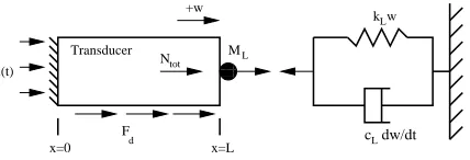
To facilitate the control design, the constitutive relations given by Eqs. (2) and (4) are used to develop a system model that quantifies forces and displacements when a magnetic field is ap-plied to the magnetostrictive transducer. The PDE model is first presented and then formulated as an ODE by the use of a finite element discretization. A damped oscillator serves as boundary conditions at the end of the actuator to represent the structure being machined. The structural model is illustrated in Fig. 1.
A balance of forces for the structural model is given by the relation [11]
ρA∂∂t2w2 =∂Ntot
000 000 000 111 111 111
+w
M
L k w
L N tot
x=L x=0
F
d c Ldw/dt
u(t)
Transducer
Figure 1. MAGNETOSTRICTIVE TRANSDUCER WITH DAMPED OS-CILLATOR USED TO QUANTIFY LOADS DURING THE MACHINING OPERATION. DISTURBANCE FORCES ALONG THE ACTUATOR ARE GIVEN BYFdAND THE CONTROL INPUT ISu(t).
where the density of the actuator is given byρ, the cross-section area is A and the displacement is denoted by w. The total force
Ntotacting on the actuator is given by the relation
Ntot(t,x) =YMA ∂w ∂x+cDA
∂2w
∂x∂t+Fmag+Fd (6)
where the elastic restoring force is given by the first term on the right hand side of the equation and a Kelvin-Voigt damping force is given by the second term. The linear elastic strain component is defined by ε= ∂∂wx. The external disturbance force is given by Fd. The coupling force Fmag represents forces generated by
applied magnetic field where
Fmag=Aa1(M−M0)2. (7)
Although the modeling framework includes disturbance loads, loads in excess of the ferromagnetic coercive stress were necessary to induce noticeable errors in the tracking performance for the system under consideration. Therefore, the disturbance loads were set to zero in the simulations.
Following Fig. (1), the boundary conditions are defined by a zero displacement at x=0 and the balance of forces at x=L
gives
Ntot(t,L) =−kLw(t,L)−cL ∂w
∂t (t,L)−ML ∂2w
∂x∂t(t,L). (8)
The initial conditions are w(0,x) =0 and∂∂wx(0,x) =0.
The PDE model given by Eq. (5) can be written in weak form and spatially discretized using finite elements to obtain an ODE system of equations. Details of the technique are given [10, 11]. This yields the following set of equations in matrix form
Mw¨+Cw˙+Kw=Fcb+fd (9)
where the matrices M∈RN×N,C∈RN×N andK∈RN×N de-note the mass, damping and stiffness matrices, respectively. The nodal displacements are denoted by w∈RN and the vectors
b,fd∈RN includes the basis functions related to the control in-put and disturbance loads, respectively. The number of finite elements is defined by N.
Equation (9) can be written in terms of a set of first order equations for developing the control law. This results in
˙
x(t) =Ax(t) + [B(u)](t) +G(t) (10)
where x(t) = [w˙,w]T should not to be confused with the coordi-nate x. The matrix A includes the mass, damping and stiffness properties of the system given in Eq. (9) and[B(u)](t)includes the nonlinear input where u(t)is defined as the magnetic field. External disturbances are given by G(t). Equation (10) is used in the following sections to develop the control law.
Control Design
First the general tracking problem is briefly summarized to provide relations used in developing the nonlinear optimal track-ing control law. The output to Eq. (10) is a linear combination of the states,
y(t) =Cx(t) (11)
where it is assumed that only displacement at the end of the trans-ducer can be measured. The cost functional
J= 1
2(Cx(tf)−r(tf))
TP(Cx(t
f)−r(tf))
+Z tf t0
H−λT(t)x˙(t)dt
(12)
is defined to penalize the measurable state and the control input where P penalizes large terminal values on the observable state,
H= 1
2
(Cx(t)−r(t))TQ(Cx(t)−r(t))uT(t)Ru(t)
+λT[Ax(t) + [B(u)](t) +G(t)]
(13)
where penalities on the observable state and inputs are given through the variables Q and R, respectively.
To determine the optimal input, the minimum of Eq. (12) must be determined under the constraint of Eq. (10). An uncon-strained optimization problem is developed by introducing the costate system [12, 13]
˙
λ(t) =−ATλ(t)−CTQCx(t) +CTQr(t). (14)
The optimal input control is determined from the stationary condition on the Hamiltonian which results in
u(t) =−R−1 ∂B
(u) ∂u
T
λ(t). (15)
The boundary conditions are applied to the state at the initial time and the final time on the costate
x(t0) =xo
λ(tf) =CTP(Cx(tf)−r(tf)).
(16)
These equations result in a two-point boundary value prob-lem that are in general challenging to solve for large N. In the fol-lowing section, linear control theory is implemented by solving the suboptimal infinite horizon problem which is often done to simplify the solution technique. Linear control theory is shown to provide poor control authority when nonlinear hysteretic ma-terial behavior is present. The two-point boundary value problem is then directly addressed in the nonlinear optimal tracking con-trol method. By introducing the constitutive behavior directly into the optimality system, it is shown that the control input ef-fectively compensates for nonlinearity and hysteresis.
Linear Tracking Control
The linear control design requires simplifying the nonlinear input given by the coupling force in Eq. (7). These terms are lin-earized by taking a Taylor series expansion about the fully mag-netized state of the material. The control input in this case is lim-ited to a small time varying input, thus only first order variations
are included in the control law. In the case of magnetostrictive materials, linearization is taken about M0.
The linearized forces are
Fmag'2Aa1M0∆M (17)
where∆M=M−M0.
A linear magnetic constitutive law is introduced such that the control input is given by an applied magnetic field
∆M=M−M0=χm∆H. (18)
The change in magnetic field is denoted by∆H whereχmis the magnetic susceptibility. This yields
Fmag'2Aa1M0χm∆H. (19)
With this approximation, the corresponding first-order sys-tem is
˙
y(t) =Ay(t) +Bu(t) +G(t) y(0) =y0.
(20)
The state constraint in Eq. (20) and the linear version of the adjoint condition in Eq. (14) yields the optimality system
"
˙
y(t)
˙
λ(t) #
= "
A −BR−1BT
−CTQC −AT #"
y(t) λ(t)
# +
" G(t)
CTQr(t) #
y(t0) =y0
λ(tf) =Πfy(tf).
(21)
For periodic, steady-state behavior, we consider the perfor-mance index
J(u) =
Z τ
0 1 2
yT(t)Qy(t) +uT(t)Ru(t)dt (22)
Since the input operator B is linear, a fundamental solution matrix is determined by solving the algebraic Ricatti equation
ATΠ+ΠA−ΠBR−1BTΠ+Q=0. (23)
The optimal control input is then defined by
u∗(t) =−R−1BT[Πy(t)−ν(t)] (24)
where the variableν(t)∈R2Nis the solution to the auxiliary dif-ferential equation
˙
ν(t) =−A−BR−1BTΠTν(t) +ΠG(t) ν(tf) =0.
(25)
In the finite time problem, the condition on the final time is substituted for an initial condition given by ν(0) =ν(τ). This approach requires restricting the disturbance force to be peri-odic whereτdenotes the fundamental period for all frequencies present. Details regarding this approach are given in [14, 15].
The suboptimal control trajectory determined by Eq. (24) is used in the following numerical examples to illustrate the need for nonlinear control when the input field reaches a magnitude that induces hysteresis.
Numerical Results: Linear Model Tracking control is demonstrated using the linear control theory to illustrate perfor-mance in tracking a reference when small or moderate to large fields are applied. The Terfenol rod is fully magnetized in the constitutive model prior to control simulation. The penalties on the state and input are given by Q=1×10¹²and R=1×10⁻¹⁰. The set of parameters given in Table 1 were used in the simula-tions.
The linear tracking control is demonstrated using a reference signal that starts at zero, ramps up, oscillates at a specified fre-quency and then ramps down to zero. The control is turned on immediately at to=0. In Fig. 2 the reference signal is limited
to small displacements (maximum displacement was 0.1 µm) so that the constitutive behavior is linear. In this case, excellent tracking is achieved as expected.
When the reference signal is increased to a level that induces hysteretic magnetic field-magnetization behavior, degradation in control authority occurs. Fig. 3 illustrates large error between
Table 1. PARAMETERS USED IN THE TRACKING CONTROL SYS-TEM.
Magnetostrictive and Damped Oscillator Parameters
kL=1.5×10⁷N/m a1=1.5×10⁻⁴N/A2
cL=1.5×10³Ns/m c1=6.1×10⁻⁵m/A
ML=0.47 kg Hc=3.3×10³A/m M0=2.75×10⁵A/m c=0.65
YM=3.0×10¹⁰N/m2 b=2.25×10⁴A/m
A=5.0×10⁻⁴m2 L=0.1 m
cD=3.7×10⁶Ns/m χm=15
the reference signal and the controlled displacement. In this sim-ulation, the reference signal is specified to have a displacement amplitude of 100 µm. The hysteretic H−M behavior is
illus-trated in Fig. 4.
Nonlinear Optimal Tracking Control
Nonlinearities and hysteresis are addressed in this section by implementing the constitutive behavior directly into the optimal-ity system previously given by Eqs. (10) and (14). The methodol-ogy follows a previous approach for active vibration attenuation of beams and plates [16, 17] . Key equations illustrating modifi-cations needed to track a reference signal are presented.
In the nonlinear model, the force determined from Eq. (7) is included in the input operator[B(u)](t)by linearizing about the bias field M0according to Eq. (17). This neglects the quadratic
0 0.5 1 1.5 2
0 0.02 0.04 0.06 0.08 0.1 0.1
Displacement (
µ
m)
Time (s)
0 0.5 1 1.5 2−0.2
0 0.2 0.4 0.6 0.8 0.8
Error
(nm
)
Commanded Displacement
Error
coupling, but includes nonlinear and hysteretic field-coupled be-havior. Details regarding this approximation are given in [18] and here in the Nonlinear Simulation Results. This yields the optimality system
"
˙
x(t)
˙
λ(t) #
= "
Ax(t) + [B(u)](t) +G(t)
−ATλ(t)−CTQCx(t) +CTQr(t) #
x(t0) =x0
λ(tf) =CTP(Cx(tf)−r(tf)).
(26)
An efficient formulation in terms of a Ricatti equation is not possible in this case due to the nonlinear nature of the input op-erator. The two-point boundary value problem is addressed by approximating Eq. (26) or the equivalent first-order system,
˙z(t) =F(t,z)
E0z(t0) = [x0,0]T
Efz(tf) = [0,0]T
(27)
where z= [x(t),λ(t)]T.
The nonlinear optimality system is now given by
0 0.5 1 1.5 2
0 20 40 60 80 100 100
Displacement (
µ
m)
Time (s)
0 0.5 1 1.5 2−30
−10 10 30 50 70 70
Error (
µ
m)
Commanded Displacement
Error
Figure 3. LINEAR TRACKING CONTROL RESPONSE WHEN MAGNE-TOSTRICTIVE NONLINEARITIES ARE PRESENT. THE CONTROLLED RESPONSE (INµm) ( ) AND THE ERROR BETWEEN THE REF-ERENCE SIGNAL AND CONTROLLED RESPONSE (INµm) ( ) IS SHOWN.
0 5 10 15 20 25 30
0 100 200 300 400
Magnetic field (kA/m)
Magnetization (kA/m)
Figure 4. CONSTITUTIVE BEHAVIOR OF THE MAGNETOSTRICTIVE TRANSDUCER USED IN THE TRACKING CONTROL SIMULATION IN FIG. 3.
F(t,z) = "
Ax(t) + [B(u)](t) +G(t)
−ATλ(t)−CTQCx(t) +CTQr(t) #
E0=
" I 0
0 0
#
, Ef =
"
0 0
−CTPC I #
.
(28)
Here I denotes an identity matrix with dimension corre-sponding to the number of basis functions employed in the spatial approximation of the state variables.
Various methods are available to approximate solutions to the system given by Eq. (27) such as finite differences and non-linear multiple shooting [19]. The finite difference approach is used here where we consider a discretization of the time inter-val [t0,tf] with a uniform mesh having stepsize ∆t and points t0,t1,···,tN=tf. The approximate values of z at these times are
denoted by z0,···,zN. A central difference approximation of the temporal derivative then yields the system
1
∆t[zj+1−zj] = 1
2[F(tj,zj) +F(tj+1,zj+1)]
E0z0= [y0,0]T
EfzN= [0,0]
(29)
Equation (29) can be expressed as the problem of finding
zh= [z0,···,zN]to which solves
F
(zh) =0. (30)Equation (30) includes the optimality system at each time step and the boundary conditions by manipulating Eq. (29). De-tails are given in [16].
A quasi-Newton iteration of the form
zk+h 1=zkh+ξkh, (31)
whereξkhsolves
F
0(zkh)ξkh=−F
(zkh), (32)is then used to approximate the solution to the nonlinear system given by Eq. (30). The Jacobian
F
0(zkh)has the formF
0(zh) =
S0 R0
S1 R1
. .. ...
SN−1RN−1
E0 Ef
(33)
where
Si=−
1
∆t "
I 0
0 I
# −1
2
"
A ∂λ∂ B[u∗i] −CTQC −AT
#
(34)
for Si. The representation for Riis similar.
Inversion of the Jacobian is required to obtain updates to the states through the iteration procedure. This is often not feasi-ble when a large number of basis functions are required to dis-cretized the structural model. In the one-dimensional rod model, this is typically not an issue, although to reduce potential numeri-cal errors in inverting the Jacobian an analytic LU decomposition is employed. The form of the equation is identical to that used in a previous investigation [16]. This gives rise to the following representation of the Jacobian,
F
0(zkh) =LU. (35)The solution of the system (32) is then obtained through di-rect solution of the lower triangular system Lζk
h=−
F
(zkh)fol-lowed by direct solution of the upper triangular system Uξk h=ζkh.
Nonlinear Simulation Results The nonlinear optimal tracking control provides enhanced control when nonlinearities and hysteresis are present. The values for Q and R previously used in the linear model are used here in the nonlinear model. The performance enhancement using the nonlinear control de-sign is demonstrated by prescribing the same reference de-signal that induced hysteresis in Fig. 4. The actuator nonlinearities are effectively compensated using the nonlinear optimal control method as shown in Fig. 5.
The tracking errors illustrated in Fig. 5 have been limited to less than 1.0 µm. These errors are primarily associated with unmodeled constitutive nonlinearities. As previously noted in the Nonlinear Optimal Track Control section, the control input is computed by approximating the strain to be proportional to the magnetization. This approximation is evaluated in Fig. 5 by computing the commanded displacement using the quadratic coupling behavior from Eq. 17. This is the primary source of error in the open loop case.
Improvements in error reduction and robustness to operating uncertainties can be achieved by feedback of perturbations in the optimal state trajectory. This has been recently addressed using a similar nonlinear optimal control design for vibration attenua-tion [17]. A hybrid method was adopted that computes the open loop nonlinear control off-line and perturbation feedback around
0 0.5 1 1.5 2 0
20 40 60 80 100
Displacement (
µ
m)
Time (s)
0 0.5 1 1.5 2−1 0 1 2 3 4
Error (
µ
m)
Commanded Displacement
Error
0 10 20 30 0
100 200 300 400
Magnetic Field (kA/m)
Magnetization (kA/m)
Figure 6. MAGNETIC FIELD-MAGNETIZATION CONSTITUTIVE BE-HAVIOR CORRESPONDING TO THE TRACKING CONTROL SIMULA-TION IN FIG. 5.
the optimal trajectory. While there are similarities to the track-ing problem, fundamental differences in the auxiliary equation (Eq. (25)) must be addressed. This is under current investigation.
Concluding Remarks
A nonlinear optimal tracking control design was developed to accurately track a reference signal when nonlinear, hysteretic magnetostrictive material behavior is present. It was shown that significant errors occur at moderate to high field inputs if the constitutive behavior is not compensated properly. This was ad-dressed by determining the nonlinear input field from the ho-mogenized energy model to compensate for nonlinear, hysteretic magnetostrictive constitutive behavior.
ACKNOWLEDGMENT
The authors gratefully acknowledge support through the Air Force Office of Scientific Research through grant AFOSR-FA9550-04-1-0203.
REFERENCES
[1] Straub, F., Kennedy, D., Domzalski, D., Hassan, A., Ngo, H., Anand, V., and Birchette, T., 2004. “Smart material-actuated rotor technology—SMART”. J. Intell. Mater. Syst.
Struct., 15, pp. 249–260.
[2] Smith, R., Bouton, C., and Zrostlik, R., 2000. “Partial and full inverse compensation for hysteresis in smart ma-terial systems”. Proc. 2000 American Control Conference, pp. 2750–2754.
[3] Smith, R., and Zrostlik, R., 1999. “Inverse compensation for ferromagnetic hysteresis”. Proc. 38th IEEE Conference
on Decision and Control, pp. 2875–2880.
[4] Duerig, T., 2002. “The use of superelasticity in modern medicine”. MRS Bull., 27(5), pp. 101–104.
[5] Ge, P., and Jouaneh, M., 1996. “Tracking control of a piezoceramic actuator”. IEEE T. Contr. Syst. T., 4(3),
pp. 209–216.
[6] Grant, D., and Hayward, V., 1997. “Variable structure con-trol of shape memory alloy actuators”. IEEE Contr. Syst.
Mag., 17(3), pp. 80–88.
[7] Smith, R., 2001. “Inverse compensation for hysteresis in magnetostrictive transducers”. Math. Comput. Model., 33, pp. 285–298.
[8] Tao, G., and Kokotovi´c, P., 1996. Adaptive control of
sys-tems with actuator and sensor nonlinearities. John Wiley
and Sons, New Jersey.
[9] Jiles, D., and Atherton, D., 1984. “Theory of the magne-tomechanical effect”. J. Phys. D. Appl. Phys., 17, pp. 1265– 1281.
[10] Smith, R., 2005. Smart Material Systems: Model
Develop-ment. SIAM, Philadelphia, PA.
[11] Dapino, M., Smith, R., and Flatau, A., 2000. “A struc-tural strain model for magnetostrictive transducers”. IEEE
T. Magn., 36(3), pp. 545–556.
[12] Bryson, A., and Ho, Y.-C., 1969. Applied Optimal Control. Blasidell Publishing Company, Waltham, MA.
[13] Lewis, F., and Syrmos, V., 1995. Optimal Control. John Wiley and Sons, New York, NY.
[14] Bittanti, S., Locatelli, A., and Maffezzoni, C., 1972. “Pe-riodic opimization under small perturbations”. In Pe“Pe-riodic
Optimization, A. Marzollo, ed., Vol. II. Udine,
Springer-Verlag, New York, pp. 183–231.
[15] DaPrato, G., 1987. “Synthesis of optimal control for an infinite dimensional periodic problem”. SIAM J. Control
Optim., 25(3), pp. 706–714.
[16] Smith, R., 1995. “A nonlinear optimal control method for magnetostrictive actuators”. J. Intell. Mater. Syst. Struct.,
9(6), pp. 468–486.
[17] Oates, W., and Smith, R. “Nonlinear optimal control tech-niques for vibration attenuation using nonlinear magne-tostricive actuators”. submitted to J. Intell. Mater. Sys. Struct.
[18] Nealis, J., and Smith, R. “Model-based robust control design for magnetostrictive transducers operating in hys-teretic and nonlinear regimes”. submitted to IEEE Trans.
Control Syst. Technol.
[19] Ascher, U., Mattheij, R., and Russell, R., 1995. Numerical