Parameter Subset Selection and Subspace Analysis Techniques Applied to a Polydomain Ferroelectric Material Phase-Field Energy Model.

ABSTRACT

LEON, LIDER STEVEN. Parameter Subset Selection and Subspace Analysis Techniques Applied to a Polydomain Ferroelectric Material Phase-Field Energy Model. (Under the direction of Dr. Ralph Smith).

In this dissertation, we illustrate parameter subset selection and subspace techniques applied to a quantum-informed Ginzburg-Landau-Devonshire theory-based phase-field energy model for mono- and polydomain ferroelectric lead titanate structures. This model may be used for character-izing multi-domain structure evolution and accounting for hysteresis and domain wall interactions, which is necessary for model-based material design.

We consider phenomenological parameters that govern attributes of the Landau polarization energy, electrostrictive energy, and gradient energy behavior. In the case of single domain structures, the model is informed by synthetic data provided by density functional theory (DFT) simulations of material electron densities. We use frequentist statistical analysis techniques to demonstrate high correlation among model parameters, which is a function of the underlying electronic structure. For the polydomain structures, we investigate free energy profiles across 180◦and 90◦twinned domain walls separating oppositely- and perpendicularly-oriented polarization at the grain level. We obtain information in this case from first-principles investigations in the literature.

We address four fundamental questions pertaining to the parameters in the model: (1) are higher-order Landau energy parameters identifiable or influential in the sense that they uniquely contribute to energy responses, (2) how much does strong parameter correlation influence sensitiv-ity analysis results in phase-field models, (3) which electrostrictive coefficients are influential to the polydomain energy response, and (4) which gradient energy parameters are most critical in the 90◦ domain wall energy? The answers to these questions are important for determining which noninflu-ential parameters may be fixed at nominal values in subsequent Bayesian inference, uncertainty propagation, and model-based design.

Parameter Subset Selection and Subspace Analysis Techniques Applied to a Polydomain Ferroelectric Material Phase-Field Energy Model

by

Lider Steven Leon

A dissertation submitted to the Graduate Faculty of North Carolina State University

in partial fulfillment of the requirements for the Degree of

Doctor of Philosophy

Applied Mathematics

Raleigh, North Carolina 2018

APPROVED BY:

Dr. Elizabeth Dickey Dr. Pierre Gremaud

Dr. Mansoor Haider Dr. Ralph Smith

DEDICATION

BIOGRAPHY

ACKNOWLEDGEMENTS

First and foremost, I would like to thank my advisor, Dr. Ralph C. Smith for his help and support during this very strenuous process. Thank you for believing in me from day one and for your unconditional kindness and dedication to my personal and professional success. Thank you also for your patience, your advice, your guidance, your expertise, your resources, and last but not least, for your friendship. To my other committee members, Dr. Elizabeth Dickey, Dr. Pierre Gremaud and Dr. Mansoor Haider, thank you for your instruction, time and expertise devoted to my preliminary exam, PhD defense and thesis dissertation.

Additionally, I would like to thank Dr. William Oates and Dr. Paul Miles for their most valuable feedback into my research, and for providing the models and DFT data, that became essential parts of my research. I would also like to thank my undergraduate research advisor Dr. Eric Forgoston for introducing me to the wonderful world of applied mathematics research, and for the investigations that helped lay the foundations for my professional career.

I owe a big part of this achievement to Mr. Bob Howitt for taking me as one of the Project 2050 scholars in the WKBJ Foundation. I am truly grateful for your support and belief in me ever since we met back in 2008. Thank you for your friendship, kindness and all those fantastic talks we’ve had over the years.

Thank you to my dear parents for instilling in me from a young age the value of getting an education, as well as for their love, encouragement and support at every stage of my life. Thank you for the core values and teachings that have shaped me into the person I am today. None of this would have ever come true if it wasn’t for you. To my brother, thank you for the great times spent together, and for being the awesome brother you are.

I’d also like to extend my gratitude to my parents-in-law for their love and encouragement throughout my graduate career. You are always there for me and I thank you from the bottom of my heart.

Finally, thank you to my fantastic wife and soul mate. Words can’t begin to describe how instru-mental you’ve been in helping me achieve this milestone. Without you by my side, crying, laughing, listening and loving me in good and bad times, none of this would have ever been possible. Thank you my dearest love.

TABLE OF CONTENTS

LIST OF TABLES . . . vii

LIST OF FIGURES. . . ix

Chapter 1 INTRODUCTION . . . 1

1.1 Identifiable and Influential Parameters . . . 4

1.2 Local and Global Sensitivity . . . 5

1.3 Active Subspace Methods . . . 6

Chapter 2 FERROELECTRIC MATERIALS . . . 8

2.1 Monodomain Structures . . . 11

2.2 Polydomain Structures . . . 11

2.3 Ferroelectric Phase-Field Model . . . 13

2.4 Density Functional Theory Calculations . . . 17

Chapter 3 PARAMETER SUBSET SELECTION and UNCERTAINTY QUANTIFICATION . . . 19

3.1 Global Sensitivity Analysis for Uncorrelated Inputs . . . 21

3.1.1 Morris Screening . . . 21

3.1.2 Variance-Based Sensitivity Analysis . . . 22

3.2 Global Sensitivity Analysis for Correlated Inputs . . . 26

3.2.1 Variance-Based Sensitivity Analysis . . . 28

3.2.2 Linearly Parameterized Problems . . . 30

3.2.3 Numerical Basis Functions Expansion . . . 32

3.3 Subset Selection using the Singular Value Decomposition . . . 34

3.3.1 SVD Subset Selection for Linearly Parameterized Models . . . 35

3.3.2 Fisher Information Matrix Analysis . . . 35

3.3.3 Random Sampling of the Sensitivity Matrix . . . 37

3.4 Active Subspace Selection . . . 38

3.4.1 Normalized Gradient Evaluations . . . 38

3.4.2 Active Subspace Construction . . . 41

3.4.3 Finding the Dimension of the Active Subspace . . . 43

3.4.4 Activity Scores . . . 44

3.5 Bayesian Inference . . . 46

3.5.1 Markov Chain Monte Carlo (MCMC) . . . 46

3.5.2 Delayed Rejection Adaptive Metropolis (DRAM) . . . 47

3.5.3 Model Calibration . . . 47

3.6 Uncertainty Propagation . . . 48

3.6.1 Sampling . . . 48

3.6.2 Energy Statistics . . . 49

Chapter 4 MONODOMAIN ENERGY ANALYSIS . . . 50

4.1 Monodomain Continuum Model . . . 52

4.2.1 Sensitivity Analysis for Uncorrelated Parameters . . . 56

4.3 Bayesian Statistical Analysis . . . 59

4.4 Sensitivity Analysis for Correlated Parameters . . . 62

4.5 Analysis Using the Fisher Information Matrix . . . 66

Chapter 5 POLYDOMAIN ENERGY MODELS . . . 71

5.1 Stored Energy Relations . . . 72

5.2 Monodomain Energy Regions . . . 74

5.3 Total Domain Wall Energies . . . 75

5.4 Parameters and Distributions . . . 76

Chapter 6 180◦POLYDOMAIN STRUCTURE ANALYSIS . . . 77

6.1 180◦Domain Wall Energy Model . . . 77

6.1.1 Model Solution Procedure . . . 79

6.1.2 Implementation . . . 81

6.2 Bayesian Inference . . . 82

6.3 Parameter Subset Selection . . . 83

6.4 Active Subspace Construction . . . 84

6.5 Uncertainty Propagation . . . 87

Chapter 7 90◦POLYDOMAIN STRUCTURE ANALYSIS . . . 91

7.1 90◦Domain Wall Energy . . . 91

7.1.1 Model Solution Procedure . . . 95

7.1.2 Implementation . . . 96

7.2 Parameter Subset Selection . . . 97

7.3 Bayesian Inference . . . 100

7.4 Active Subspace Construction . . . 101

7.5 Uncertainty Propagation . . . 103

Chapter 8 CONCLUSIONS. . . .108

BIBLIOGRAPHY . . . .111

APPENDIX . . . .116

LIST OF TABLES

Table 4.1 Elastic coefficients obtained from[24]. . . 51 Table 4.2 Nominal values for the polarization parametersθPand the stress component

parametersθ_σ, defined in (4.9) and (4.10), respectively. The nominal values were obtained from a least-squares optimization of the outputs (4.12). . . 54 Table 4.3 Sobol’ sensitivity indicesSi,STi, Morris screening measuresµ

∗

i,σ∗iand Pearson correlation coefficientsρa l l,ρi n f for the Landau energy phenomenological parametersθP (4.9). Note thatρi n f indicates Pearson correlation coefficients when only presumed influential parameters are sampled while all others are fixed. The shaded cells correspond to significant indices, measures and coeffi-cients. . . 59 Table 4.4 Sensitivity indices for total contributionsSrn constructed using the component

functionsfrn for the Landau energy parametersθP. The A’s and N’s represent sensitivity indices derived from the analytical and numerical determination of the component functions, respectively. The indices correspond to the order specified byθP= [α1,α11,α12,α111,α112]. The shaded cells designate significant indices. . . 67 Table 4.5 Sensitivity indices for total contributionsSrn constructed using the component

functionsf_rn for the normal stress parametersθ_{σn s}. The indices correspond to the order specified byθ_{σn s}= [q11,q12,σR11,σR22,σ33R]. The shaded cells corre-spond to significant indices. . . 68 Table 4.6 Sensitivity indices for total contributionsS_rn constructed using the component

functionsfrn for the shear stress parametersθσs. The indices correspond to the order specified byθ_σs= [q44,σR₂₃]. . . 68 Table 4.7 Results from Algorithm 3.3.2, to determine unidentifiable parameters inθP

(4.9) for the polarization energyuP(4.3). . . 69 Table 4.8 Results from Algorithm 3.2 to determine unidentifiable parameters inθ_σ(4.10)

for the normal and shear stress componentsσn sandσs (4.8). . . 70 Table 6.1 List of parameters used in solution and evaluation of the domain wall energy

(6.5), along with corresponding units. The parametersθ₁₈₀M D are appropriately scaled from Table 4.2 to reflect the new unit system employed here. . . 81 Table 6.2 Units of measurement used in the 180◦domain wall model for energy, length,

charge, and voltage . . . 82 Table 6.3 Results from Algorithm 3.3.2 with the global sensitivity matrix (3.44) to

deter-mine noninfluential parameters inθ180(6.6) for the 180◦domain wall energy E180◦(6.5). . . 84 Table 6.4 Mean relative errors (MRE) for response surfaces considering 1-, 2-, and

3-dimensional active subspaces for the mode responseE180◦. . . 85 Table 6.5 Energy test statistic and critical values forα=0.05,α=0.10 with respect to

Table 7.1 Nominal values for parametersθ90 with respect to the domain wall model energy modelE₉₀◦(θ90). . . 97 Table 7.2 Results from Algorithm 3.3.2 with the global sensitivity matrix (3.44) to

deter-mine noninfluential parameters inθ90(7.19) for the 90◦domain wall energy E₉₀◦(7.18). . . 99 Table 7.3 Mean relative errors (MRE) for response surfaces considering 1-, 2-, 3-, and

4-dimensional active subspaces for the model responseE90◦. . . 102 Table 7.4 Energy test statistic and critical values forα=0.05,α=0.10, when sampling the

LIST OF FIGURES

Figure 1.1 Schematic of the steps in uncertainty quantification, most associated with this dissertation. This is a partial diagram of the complete schematic given in [51]. . . 3 Figure 1.2 Illustration ofy =f(θ)for (a) identifiable, (b) unidentifiable, and (c)

nonin-fluential parametersθ. Plotted after[27]. . . 4 Figure 1.3 Illustration of (a) a highly influential parameterθ1and (b) minimally

influen-tial parameterθ2. (c) Minimally influential parameterθ3having large local derivative values. Plotted after[27]. . . 5 Figure 2.1 (a) Dependence of the Curie temperature TC on the molar fraction x of

PbZrO3, and morphotropic phase boundary separating rhombohedral from tetragonal structures. (b) Dependence of the piezoelectric coupling coeffi-cient on the molar fractionx. Plotted after[22]. . . 9 Figure 2.2 Schematic of ferroelectric material grains depicting 180◦and 90◦domains

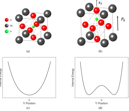
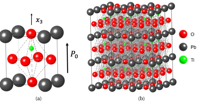
and domain walls. Polarization is randomly oriented in the grains. Plotted after[52]. . . 10 Figure 2.3 Atomic structure unit cell of lead titanate (PbTiO3), with polarization oriented

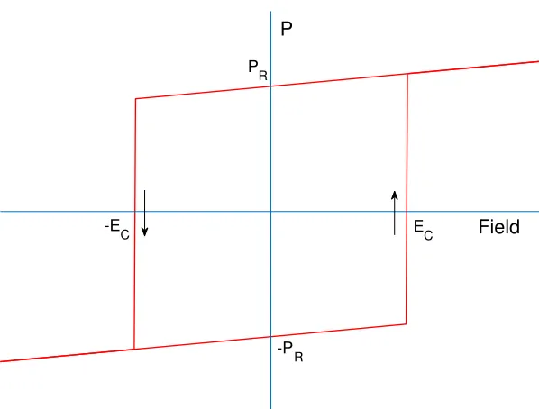
in thex3direction. (a) Cubic form of PbTiO3in the paraelectric phaseT >TC. (b) Tetragonal structure of PbTiO3, along with spontaneous polarizationP0in thex3direction. (c) PbTiO3internal energy as a function of the Ti position in the paraelectric phaseT >TC, and (d) in the ferroelectric phaseT <TC. . . 12 Figure 2.4 Hysteretic field-polarization relation produced by ferroelectric switching

mechanisms, when applied electric fields are larger thanEC in magnitude. The remanence polarizationPRoccurs when the applied electric field is zero, where the linear and reversible direct and converse piezoelectric effects are applicable. . . 13 Figure 2.5 (a) Ferroelectric phase for PbTiO3, with polarization oriented in thex3

direc-tion. (b) Single domain structure for PbTiO₃. . . 14 Figure 2.6 (a) 180◦and (b) 90◦polydomain structures of polarization orientation.

Do-mains are separated by corresponding domain walls or boundaries. We depict a new coordinate system for the 90◦_{polydomain structure. As detailed in}

Sec-tion 2.2, this new 45◦-rotated coordinate system is denoted by(s,r,x3), with the domain wall positioned ats=0. . . 14 Figure 2.7 Polarization states at which DFT energy and stresses were calculated in the

computational study of[33]. . . 18 Figure 4.1 Input polarization values ofP2andP3obtained from the DFT analysis

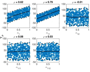
imple-mented in[33], and employed in the Landau polarization energy (4.3). . . 53 Figure 4.2 Scatterplots, Pearson correlationsρgiven by (3.7), means, and two standard

Figure 4.3 Pearson correlations of sampled (a)α1, (b)α11against each of 500 realiza-tions ofYP (4.13), with all other parameters inθP also sampled and onlyα1, α11sampled. Pearson correlation coefficientsρfor each parameter are also presented. The labels (—) and (- - -) denote the means and two standard deviations for the cases where all parametersθP are sampled to obtain the responses shown by (o), and only parametersα1,α11are sampled to obtain the responses shown by (+). . . 58 Figure 4.4 Chain of accepted sampled Landau energy parameter values with respect to

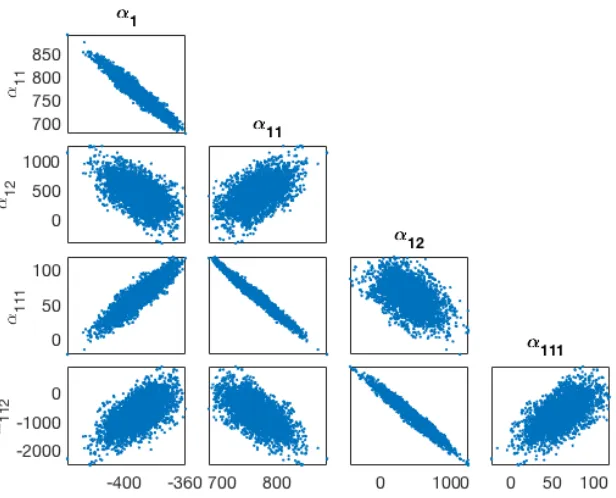
DFT simulations in[33], obtained using 1×104iterations. . . 60 Figure 4.5 Pairwise correlation among the Landau energy parameters (4.9). Strong

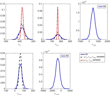
cor-relation observed between the lower- and higher-order parameters. . . 61 Figure 4.6 Posterior densities obtained via Bayesian calibration ofY_p(θP)in when (i)

sampling all the parameters, (ii) samplingα1,α11,α111withα12,α112fixed, and (iii) samplingα1,α11withα111,α12,α12fixed. . . 62 Figure 4.7 (a) First, (b) second, (c) third, (d) fourth and (e) fifth-order component

func-tions constructed using the analytical method (- -) and the numerical method (—) forθP in (4.13) withm =4 subintervals for the Cubic B spline basis functions. . . 64 Figure 4.8 (a) First, (b) second, (c) third, (d) fourth and (e) fifth order component

func-tions constructed using the analytical method (- -) and numerical method (—) forθ_{σn s} in (4.14) withm=4 subintervals. . . 65 Figure 4.9 First-order component functions constructed using the analytical method

(--) and numerical method (—) forθ_σs in (4.15) withm=4 subintervals. . . 65 Figure 4.10 Comparison of analytical and numerical methods obtain (a) first-order and

(b) total sensitivity indices for (4.13). . . 67 Figure 4.11 Comparison of analytical and numerical methods to obtain (a) first-order

and (b) total sensitivity indices for (4.14). . . 69 Figure 4.12 Comparison of analytical and numerical methods to obtain (a) first-order

and (b) total sensitivity indices for (4.15). . . 69 Figure 6.1 Comparison of analytic, finite difference and MATLAB

bvp4c.m

solution 180◦domain wall energy system. From top left to bottom right, 180◦ domain wall energy density solution, polarizationP3in thex1direction, strain "11in thex₁direction, and polarization gradient in thex₁direction as we cross the 180◦domain wall. . . 82 Figure 6.2 (a) Chain of accepted values and (b) kernel density estimation (kde) for the

parameterg₄₄obtained from the Bayesian uncertainty analysis with respect toE180◦. . . 83 Figure 6.3 Singular values obtained from the active subspace determination forE180◦

assumming uniform (3.47) and normal (3.49) distributions for parameters θ180. The shading indicates two standard deviations from the sample mean. . 85 Figure 6.4 Response surfaces forE180◦constructed based on a (a) one-dimensional and

Figure 6.5 Activity scores for the model response E180◦ assuming uniform (3.47) and normal (3.49) parameter distributions, and a (a) one-dimensional and (b) two-dimensional active subspace. . . 86 Figure 6.6 Uncertainty propagation of the (a)θ180model inputs and (b)θ₁₈₀s e n sinfluential

inputs on the energy densityu₁₈₀(x₁)−u₀. . . 88 Figure 6.7 (a) Peak residuals obtained for the different credible intervals (CI) peaks of

Figure 6.6(a) subtracted by the peaks of Figure 6.6(b). (b) 50% CI peak residuals obtained from the 50% CI peaks of Figure 6.6(a) subtracted by the peaks of Figure 6.6(b). . . 88 Figure 6.8 (a) Histogram and (b) probability density of the 180◦ domain wall energy

u180(0)−u0distributions with respect to the case where the uncertainties of all parametersθ180are propagated, as compared with the case where only the uncertainties of parametersθ₁₈₀s e n s are propagated. In (c) and (d) parame-ters were sampled directly from the chains in the monodomain analysis of Section 4.3 and[33], and the uncertainty analysis of Section 6.2. . . 89 Figure 6.9 Energy test statistic replicates for the analysis of theu180(0)−u0distribution

considering a (a) normal distribution and (b) direct sampling from the mon-odomain chains of[33]for the Landau and electrostrictive parameters in θ180. . . 90 Figure 7.1 Comparison of finite difference

fsolve.m

bvp4c.m

solution of the 90◦domain wall energy system. From top left to bottom right, 90◦domain wall energy density solution, polarizationPs in thesdirection, polarizationPr in thesdirection, and polarization gradientsPs,s andPr,s in thesdirection as we cross the 90◦_{domain wall. . . 98}

Figure 7.2 (a) Chain and (b) kernel density estimation for the parameterg11, obtained from the implementation of the DRAM algorithm[18]. . . 100 Figure 7.3 Singular values obtained from the active subspace determination forE₉₀◦

assuming normal (3.49) and uniform (3.47) distributions for parametersθ90. The shaded area around the singular values corresponds to two standard deviations. . . 101 Figure 7.4 Response surface forE90◦constructed based on a (a) one-dimensional and

(b) two-dimensional active subspace. . . 102 Figure 7.5 Activity scores for the model responseE₉₀◦assuming normal (3.49) and

uni-form (3.47) parameter distributions, and a (a) one-dimensional and (b) two-dimensional active subspace. The errorbars indicate two standard deviations from the mean. . . 103 Figure 7.6 Uncertainty propagation of the (a)θ90model inputs and (b)θ₉₀s e n sinfluential

inputs on the energy densityu90(s)−u0, assuming a normal distribution for the parameters. In (c) and (d) we sample directly from the monodomain chains in[33]for the Landau and electrostrictive parameters. . . 105 Figure 7.7 Peak residuals obtained for the different credible intervals (CI) peaks of

Figure 7.8 (a) Histogram and (b) probability density of the 90◦ domain wall energy u₉₀(0)−u₀distributions with respect to the case where the uncertainties of all parametersθ90are propagated against the case where only the uncertainties of parametersθ₉₀s e n s are propagated. In (c) and (d) we sampled directly from the chains obtained in the monodomain analysis reproduced in Chapter 4 and obtained from[33]. . . 106 Figure 7.9 Energy test statistic replicates for the statistical analysis of theu90(0)−u0

CHAPTER

1

INTRODUCTION

“If we knew what it was we were doing, it would not be called research, would it?”

- Albert Einstein

Sensitivity analysis and uncertainty quantification play pivotal roles for scientists and engineers using models to predict physical phenomena with quantified uncertainties. Specifically, sensitivity analysis or parameter subspace analysis comprises a critical first step to isolate subsets or sub-spaces of parameters that are identifiable in the sense that they are uniquely determined by data as influential on measured responses. Noninfluential or nonidentifiable parameters are fixed at nomi-nal values before subsequent Bayesian inference to quantify input uncertainties and uncertainty propagation to compute intervals for quantities of interest.

rela-tions, as detailed in[33]. However, using quantum calculations to inform a macroscopic continuum domain introduces uncertainty into the model that may have significantly different parameter uncertainties[27]. The techniques described in Chapter 3 are focused on addressing and quantifying this uncertainty.

Specifically, the energy model we consider in this dissertation is composed of classical energy functionals for the mechanical energy, Landau polarization energy, electrostrictive energy and gradient energy. The attributes of these functionals are governed by unknown phenomenological parameters that must be estimated prior to their employment in model-based material design. For example, the sixth-order Landau polarization energy

uP(P) =α1(P12+P 2 2 +P

2

3) +α11(P 2 1 +P

2 2 +P

2 3)

2_+α12(P2 1P

2 2 +P

2 1P

2 3 +P

2 2P

2 3)

+α111(P₁6+P₂6+P₃6) +α112P₁4(P₂2+P₃2) +P₂4(P₁2+P₃2) +P₃2(P₁2+P₂2)

+α123P₁2P₂2P₃2

(1.1)

is governed by the phenomenological parametersθP= [α1,α11,α12,α111,α112,α123], specifying the non-convex energy potential as a function of the polarizationP= [P1,P2,P3].

To facilitate the employment of phase-field models in material design, we focus on two major issues pertaining to these parameters. First, we determine which of the parameters are identifiable or influential in the sense that they uniquely contribute to energy responses. Secondly, we determine the actual parameter values that dictate specific material behavior and the associated uncertainties in these values. Both of these issues are addressed in Chapter 4 for single domain energy responses, and in Chapters 6-7 for polydomain energy responses.

For the Landau polarization relation (1.1), we employ sensitivity analysis to determine whether the sixth-order model is necessary to approximate quantum calculations or whether a fourth-order model will suffice. In classical global sensitivity analysis methods, parameters are assumed to be uniformly and independently distributed in the absence ofa prioriknowledge of the underlying parameter distribution. This assumption is made to avoid introducing unintentional biases. How-ever, we show that Landau parameters are strongly correlated and determine how the correlation influences sensitivity analysis results.

Domain walls have long been evidenced to produce attractive properties of ferroelectric materi-als, such as high piezoelectric and dielectric constants[5, 32, 57]. The parameters most associated with electromechanical effects of polarization and strain in the Landau-Ginzburg energy are the coefficientsq11,q12andq44governing the electrostrictive energy

uC =−q11 "11P12+"22P 2 2 +"33P

2 3

−q12

"11 P₂2+P₃2+"22 P₁2+P₃2+"33 P₁2+P₂2

−q44("12P1P2+"13P1P2+"23P2P3).

Figure 1.1Schematic of the steps in uncertainty quantification, most associated with this dissertation. This is a partial diagram of the complete schematic given in[51].

When transitioning through the 180◦_{and 90}◦_{domain walls, polarization and strain evolution are}

further dependent on high-order coupling between the electrostrictive coefficients and the Landau energy parameters in (1.2), as well on polarization gradient exchange parameters as detailed in Chapters 2, 5, 6 and 7. Consequently, we determine which parameters are noninfluential with respect to the polydomain energy response, to be fixed for subsequent Bayesian inference and uncertainty propagation. We provide a more detailed introduction to ferroelectric materials and phase-field energy models in Chapter 2.

θ θ

y y y

(a) (b) (c)

1 2

θ _θ θ

Figure 1.2Illustration ofy=f(θ)for (a) identifiable, (b) unidentifiable, and (c) noninfluential parameters

θ. Plotted after[27].

1.1

Identifiable and Influential Parameters

We first define identifiable and influential parameters. We will use this terminology throughout this dissertation to describe parameters that do not significantly influence model responses.

Consider the general input-output relation

Y =f(Θ),

whereΘ= [Θ1, . . . ,Θp]are random variables representing inputs, or parameters, andθ= [θ1, . . . ,θp] are realizations of those random variables. HereY andy are also corresponding random variables and realizations for the responses. For example, in the polarization energy (1.1),Θ=ΘP are the phenomenological parameters,f denotes the sixth-order relation, andy =u_P(P)denotes the energy for a specified polarization value.

The concept of identifiability is defined as follows. Parametersθ= [θ1, . . . ,θp]are identifiable atθ∗if f(θ) =f(θ∗_{)implies thatθ=θ}∗_{for realizationsθ in an admissible parameter space}

Q. We

denoteI(θ)as the identifiable subspace. The parametersθ are identifiable with respect to this space, if it holds for allθ∗∈I(θ). The unidentifiable subspaceN I(θ)is the orthogonal complement ofI(θ), with respect to the Euclidean inner product. Unidentifiable parameters must be fixed at nominal values for model calibration using outputsy, whereas the identifiable parameters may be uniquely determined from observations. We illustrate an example of identifiable and unidentifiable parameters in Figure 1.2(a) and (b), respectively.

In the same context, we define parameters θ to be noninfluential on the spaceN I(θ)if

|f(θ)−f(θ∗)|< " for allθ andθ∗ ∈ N I(θ). Likewise,I(θ)is the influential parameter space and orthogonal complement ofN I(θ), in the admissible parameter spaceQ. Similar to

unidenti-fiable parameters, noninfluential parameters can be fixed for subsequent model calibration and uncertainty propagation. We illustrate an example of a noninfluential parameter in Figure 1.2(c).

3

(a) (b) (c)

y y y

a _{a a}

b b b

θ₁ θ₂ θ

Figure 1.3Illustration of (a) a highly influential parameterθ1and (b) minimally influential parameterθ2. (c) Minimally influential parameterθ3having large local derivative values. Plotted after[27].

θ2if perturbations inθ1produce greater variability iny than perturbations inθ2. We illustrate highly and minimally influential parameters in Figure 1.3(a) and (b).

1.2

Local and Global Sensitivity

Through the use of parameter subset selection techniques, such as local and global sensitivity analysis, we determine which parameters are most influential in a model. We can then use this information to fix those parameters, which do not significantly influence the model, in the sense that their perturbations are only minimally reflected in the model response.

Local sensitivity analysis concerns the change in a model output or response with respect to local changes in nominal parameter values. A measure of local sensitivity is obtained by evaluating the partial derivatives

∂f

∂ θ(θ∗). (1.3)

The limitations in using local sensitivity analysis to determine a parameter subset suitable for uncertainty quantification are that we do not broadly account for uncertainties and parameter interactions across the entire parameter space. For example, as illustrated in Figure 1.3(c), the parameterθ3is noninfluential when considered throughout the admissible parameter space, but has large derivatives locally at certain nominal values. Morris screening (defined in Section 3.1) partially addresses this issue by statistically averaging derivative approximations at multiple nominal values[35].

This motivates global sensitivity analysis, in the sense that the uncertainties in the model re-sponse are more broadly apportioned to the uncertainties in the model inputs. Rather than studying the sensitivity of the modely =f(θ), to local perturbations aboutθ∗_{, we consider associated}

In Chapter 3, we introduce several global sensitivity analysis methods used in our investigation. This includes variance-based global sensitivity analysis, based on[46, 53], as well as the approximated gradient-based methods of[35]. We compare and contrast the methods and provide an alternative approach for performing variance-based global sensitivity analysis when model parameters are strongly correlated. This method, based on the theory of[29], is motivated by cases where the assumption of independently and uniformly distributed parameters is violated and hence can yield incorrect sensitivity results.

1.3

Active Subspace Methods

In some cases, influential or identifiable parameter spaces can include linear combinations of parameters. In such scenarios, it is useful to consider directions in the admissible parameter space, not aligned with particular coordinate axes, corresponding to individual parameter values. Here we often discover that the function may vary most dominantly, with respect to directions dictated by linear combinations of the parameter values, as detailed in[8]. Typically this includes a small number of directions, and one can project onto this low-dimensional space by employing a linear transformation. This provides us with the capability to use linear algebra properties to determine an influential subspace. As this subspace contains the most influential or “active” directions in the admissible parameter space, we refer to it as theactive subspace. The active subspace is additionally less susceptible to unknown distributions, facilitating analysis where parameter densities are not knowna priori.

The active subspace is determined by the construction of a gradient, or approximate gradient, matrixG, containing evaluations of the function gradient with respect to random parameter values, and its corresponding singular value decompositionG=WΣVT, as proposed in[1, 8, 44]. Alterna-tively, a QR decomposition may also be used. The projection of the original input parametersθ onto the active subspace is obtained by the relation

y=WT₁θ.

Here,yare the active variables andW1represents the firstm singular vectors, wherem is the dimension of the active subspace. The orthogonal projectionz=WT₂θ represents the inactive subspace projection, where perturbations in these directions are reflected minimally in the original model response. We provide more details about the construction and dimension selection of the active subspace in Chapter 3.

model response, as a function of the active variables. This greatly reduces the computational cost, since it many cases, the response surface is constructed from a simple regression analysis, and is a function of only a few active variables.

One can also exploit information from the SVDG=WTΣVT, to construct global sensitivity metrics

ai= m

X

j

λjw_i,j2 , i=1, . . . ,p

CHAPTER

2

FERROELECTRIC MATERIALS

Ferroelectric materials are characterized by the presence of spontaneous polarization in the ab-sence of electric fields, at temperatures below the Curie pointTc. The materials exhibit tetragonal, orthorhombic or rhombohedral phases at these temperatures, where the orientation of polarization is determined by the coordinates of atoms in the unit cell. Additionally, this polarization orientation can be reversed by the application of an electric field or mechanical stress.

Ferroelectric materials are closely related to pyroelectric and piezoelectric materials. Pyroelectric materials develop a voltage due to an increase or decrease in temperature, and the polarization changes as a result. Many piezoelectric materials serve as actuators and sensors in the sense that they develop mechanical forces due to an applied electric field, and conversely develop a voltage due to an applied external force. In particular, they are characterized by the ability to produce a change in polarization when subjected to mechanical stress. This is termed the direct piezoelectric effect. Alternatively, the material can produce mechanical strain in response to an applied electric field, yielding the converse piezoelectric effect.

0 50 100 0

250 500

T (

° C)

Cubic

Tetragonal

Morphotropic Phase Boundary

T_C

Rhombohedral

Orthorhombic

PbZrO₃ Mol % PbTiO₃ PbTiO₃

0 50 100

0 0.05 0.1 0.15 0.2 0.25 0.3 0.35 0.4

Piezoelectric Coupling Coefficient

PbZrO₃ Mol % PbTiO

3 PbTiO3

(a) (b)

Figure 2.1(a) Dependence of the Curie temperatureTC on the molar fractionxof PbZrO3, and mor-photropic phase boundary separating rhombohedral from tetragonal structures. (b) Dependence of the piezoelectric coupling coefficient on the molar fractionx. Plotted after[22].

high energy efficiency rates and complementary direct and converse effects, provide excellent properties for the development of energy harvesting circuits[55], flow control transducers[2, 26], ultrasound transducer devices for biomedical imaging[36], and flying and ambulatory microrobots [20, 40, 62, 63].

The material studied, and of main interest in this dissertation, is PbTiO3. This, along with PbZrO3or lead zirconate, is a main component in PZT. These materials are present in PZT as part of the molar fraction x of Zr in PbTi1−xZrxO3. The determination ofx is based on the desired optimal electromechanical properties for specific engineering applications. As depicted in the phase diagram of Figure 2.1(a), PbZrO3 exhibits a orthorhombic phase at temperatures below the Curie point, whereas PbTiO3exhibits a tetragonal phase. Note that PZT is advantageous for transducer engineering applications due to its strong electromechanical coupling constant near the morphotropic phase boundary, as illustrated in Figure 2.1(a)-(b). Since lead titanate is a critical component in PZT, and density functional theory (DFT) calculations (Section 2.4) are facilitated for PbTiO3as compared with PbZrO3[37], we focus our attention on this material throughout this dissertation.

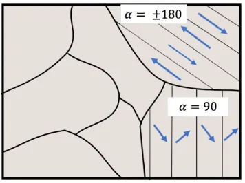
Figure 2.2Schematic of ferroelectric material grains depicting 180◦and 90◦domains and domain walls. Polarization is randomly oriented in the grains. Plotted after[52].

transducer designs.

A disadvantage of PZT is the presence of lead, which is toxic in the environment. As a result, significant effort has focused on developing new materials that can replace lead-based materials[21, 25], while maintaining the high performance required for applications. To develop new materials, it is critical to understand why lead-based ones are so effective. This starts with experimental and computational investigations ranging in scales from the material devices down to the micro-sized grains, nanoscale domains and atomic structure of the materials. A complete-structure evolution investigation thus requires the development of effective and efficient methods for characterizing free energy behavior within material grains. Energy relations across multiple scales can then be incorporated into homogenized energy frameworks, such as the one in[50, 52], to develop model-based control algorithms for bulk materials.

2.1

Monodomain Structures

In terms of its unit cell, lead titanate exhibits a perovskite structure, with lead atoms occupying the A site and the titanium atom the B site. The material is cubic (paraelectric phase) above the Curie temperature TC and it achieves its tetragonal (ferroelectric) phase when cooled below TC. The material’s internal energy for the paraelectric phase exhibits one unique minimum, whereas it exhibits two minima depending on the position of the Ti atom for its tetragonal phase, thereby determining the polarization orientation. A plot of the material energy profiles, along with the corresponding perovskite crystal structure is given in Figure 2.3. A macroscopic polarization is oriented in thex3direction as dictated by the shift in the center Ti atom. When sufficient energy in the form of elastic or electrostatic forces is applied, the ion moves across the unstable equilibrium to the other potential well, thus producing a dipole switch, and a polarization jump at the macroscopic scale. In particular, the dipoles switch may be caused by the application of electric fields larger in magnitude than the coercive fieldE_C, denoting the field required to reduce polarization to zero. These switching mechanisms produce hysteresis and saturation nonlinearities, as illustrated in Figure 2.4. This behavior may be characterized by the implementation of the ferroelectric phase-field models discussed in Section 2.3.

When discussing monodomain structures, we refer to twinned unit cells with polarization orientation in the same direction within a single crystal. For a positive polarizationP3in thex3 direction, we plot the unit cell along with a single domain in Figure 2.5. In later chapters, we consider polarization rotation fromx3tox2, and determine free energy associated with this domain structure evolution, informed by density functional theory (DFT) calculations as introduced in Section 2.4. Domains with polarization oriented in opposite directions or perpendicular toP₃are separated by domain walls or boundaries as detailed in the next section.

2.2

Polydomain Structures

The cooling of the material leads to the formation of many irregular nanoscale domain structures of polarization orientation. This produces one of the main sources of uncertainty at the micro-sized grain level, where nonlinearities are caused by many polarization-oriented structures. As depicted in Figure 2.2, each grain is composed of 180◦and 90◦domains in which oppositely- or perpendicularly-oriented polarization is separated by domain walls or boundaries. We illustrate a 2-D example of 180◦_{and 90}◦_{polarization domains and domain walls in Figure 2.6. Here, we consider the domain}

(a) (b)

0

Ti Position

Internal Energy

0

Ti Position

Internal Energy

(c) (d)

Figure 2.3Atomic structure unit cell of lead titanate (PbTiO3), with polarization oriented in thex3 direc-tion. (a) Cubic form of PbTiO3in the paraelectric phaseT>TC. (b) Tetragonal structure of PbTiO3, along with spontaneous polarizationP0in thex3direction. (c) PbTiO3internal energy as a function of the Ti position in the paraelectric phaseT>TC, and (d) in the ferroelectric phaseT<TC.

in Figure 2.6(b), with the domain wall positioned ats=0. We present more details in Chapter 6. We determine energy densities, total energy and corresponding model parameter sensitivities and uncertainties associated with 180◦and 90◦domain walls. Note that our analysis focuses on Pb-centered 180◦domain walls that lie on Pb-O planes, whereas we consider Pb-Ti-O-centered 90◦ domain walls. As noted in[32], there is no sharp distinction between specific planes used for 90◦

Field P

P R

-E

C EC

-P R

Figure 2.4Hysteretic field-polarization relation produced by ferroelectric switching mechanisms, when applied electric fields are larger thanEC in magnitude. The remanence polarizationPR occurs when the

applied electric field is zero, where the linear and reversible direct and converse piezoelectric effects are applicable.

terms of the total domain wall energy, its values are reported to be 132 mJ/m2and 50 mJ/m2, for the 180◦and 90◦domain wall structures respectively[56].

2.3

Ferroelectric Phase-Field Model

(a) (b)

Figure 2.5(a) Ferroelectric phase for PbTiO3, with polarization oriented in thex3direction. (b) Single domain structure for PbTiO3.

(a) (b)

Figure 2.6(a) 180◦and (b) 90◦polydomain structures of polarization orientation. Domains are separated by corresponding domain walls or boundaries. We depict a new coordinate system for the 90◦polydomain structure. As detailed in Section 2.2, this new 45◦-rotated coordinate system is denoted by(s,r,x3), with the domain wall positioned ats=0.

associated polarization and strain as the independent variables. Characterization of the electronic behavior via order parameters and nonlinear stress effects induced by domain wall structures produces uncertainty in the model response and parameters, due to the incorporation of quantum-scale effects into a continuum domain.

propagation for free energy models informed by DFT simulations for lead titanate. These quantum-based calculations provide computational measures of polarization and free energy. Results obtained from[33]and other literature reference values[32, 56]are treated as high-fidelity calculations to inform our models for characterization of single- and multi-domain energy structures.

For linear operating regimes, corresponding to low input electric field levels, energy functionals, which incorporate linear electromechanical coupling, accurately characterize domain structure evolution. As detailed in[50], to incorporate additional ferroelectric hysteresis or phase transitions, it is necessary to quantify internal processes such as dipole switching or entropic effects in the absence of stresses or electromechanical coupling. To quantify this behavior, one can employ the Helmholtz energy relation

ψ(",P,T) =1 2Y

P_"2

−a1"P −a2"P2+ψ0(T) +α1(T −TC)P2+α2P4+α3P6. (2.1)

HereYP_{is the Young’s modulus at constant polarization,a}

1anda2denote positive coupling coeffi-cients,α1andα2are positive constants, andψ0(T)includes temperature effects independent of strain"and polarizationP. In comparison with energy functionals for linear operating regimes, re-lations such as (2.1) consider nonlinear electromechanical coupling terms, whose minima quantify polarization and strain densities in the absence of applied fields.

Whereas the Helmholtz energy relation (2.1), provides mechanisms for characterizing hysteresis in single crystal material compounds, we require a model that incorporates effects due to domain wall interactions as well as polarization and stress-dependent switching behavior across multiple domains. This is accomplished by using the Ginzburg-Landau theory for characterizing free energy [14], in which domain wall interactions are incorporated via the inclusion of polarization gradient terms of the form∂_∂P_x. As illustrated in the work by Shu and Bhattacharya[49], Smith[50], Zhang and Bhattacharya[65], and further detailed in Chapter 4, the gradient energy terms incorporate local polarization changes due to domain wall effects. In addition, free energy is assumed to be nonlinearly dependent on quadratic, quartic and sextic polarization terms, and induced by electrostriction and a strain relationship motivated by Hooke’s law.

In general, the phenomenological internal stored energy is divided into mechanical, polariza-tion, electrostrictive, and gradient energy terms. Since one electronic coordinate vector is used to approximate the internal electronic structure in the DFT studies in[37], a polarization order parameterPis used to represent the state. Thus, we treat polarizationPand strainεas independent variables in the system. The 3-D stored free energy in the material polydomain system is thus given by

energyuC and gradient energyuG. For the analysis of the monodomain structures, we consider the first three terms on the right hand side of system (2.2), whereas we include the gradient energy term for analysis of the polydomain structures. Additionally, a residual energy termuR is considered to compare with results from DFT studies where the unit cell is held fixed with respect to a reference cubic state. We provide more details about the residual energy in Chapter 4.

Our goal is to determine which phenomenological parameters are influential or identifiable in the sense that they are uniquely determined by available data as detailed in Section 1.1. In the case of the Landau energy

u_P(P) =α1 P2

1 +P22+P32

+α11 P2

1 +P22+P32

2

+α12 P2

1P22+P22P32+P12P32

+α111 P₁6+P₂6+P₃6+α112P₁4 P₂2+P₃2+P₂4 P₁2+P₃2

+P₃4 P₁2+P₂2+α123P₁2P₂2P₃2,

(2.3)

one seeks to determine whether or not a sixth-order expansion is necessary as compared to using a fourth-order expansion for characterization of phase transition and monodomain structure evolu-tion. Relation (2.3) is analogous to the fifth, sixth and seventh terms in (2.1), with the exception that (2.3) incorporates 3-D polarization effects. Additionally, in (2.3) we consider a temperatureT <TC such thatα1is an unknown phenomenological parameter whose value is less than zero.

The gradient energy density is taken to be

uG(Pi,j) = g₁₁

2 P

2 1,1+P

2 2,2+P

2 3,3

+g12 P1,1P2,2+P1,1P3,3+P2,2P3,3

+g44 2

”

P_1,2+P_2,12+ P_1,3+P_3,12+ P_2,3+P_3,22—,

(2.4)

whereg11,g12andg44denote the exchange parameters and

Pi,j= ∂P_i ∂xj

is the polarization gradient. For 180◦and 90◦domain wall polarization effects, we seek to determine the influential exchange parameters in (2.4), in the sense that their uncertainties directly contribute to the uncertainty in the response.

2.4

Density Functional Theory Calculations

Density functional theory (DFT) calculations describe the quantum behavior of atoms and molecules through solutions of the Schrödinger equation. As such, DFT is used to determine many structure-dependent properties for collections of atoms. Of particular importance is the energy calculation of atoms and the change in energy as these atoms are moved. To effectively determine these energy states, solutions of the atoms’ electron densities are required. The ground state energyE of the electrons, in Schrödinger’s equation, is then expressed as the functionalE[n(r)], wheren(r)is the electron density for a particular 3-coordinate position vectorr. This motivates the namedensity functional theory. More details about the theory behind DFT are provided in sources including[48, 64, 66]

For the ferroelectric phase-field model studied in this dissertation, DFT informs the continuum scale Landau energy and stresses associated with several uniform polarization states in lead titanate. For the monodomain structures, we use the DFT calculations from[33], treated as high fidelity results, to quantify the uncertainty in the Landau energy parameters and electrostrictive energy coefficients, in the stored energy (2.2). Model parameter uncertainty is present since we are going from a quantum DFT calculation to a continuum framework description using polarization as the order parameter.

As detailed in[33, 37], the DFT calculations for the monodomain structure were performed using ABINIT 7.0.5[16]for lead titanate (PbTiO₃). Starting with the centrosymmetric atomic configuration, atoms were linearly incremented, yielding an equilibrium tetragonal state and a double well potential energy. To estimate the full three-dimensional energy surface, atomic displacements under internal atomic shearing were used, quantifying polarization not aligned with the spontaneous polarization direction. Note that the corresponding polarization for the atomic displacement configurations was obtained using the Berry phase approach[43]. This yields the polarization rotation profiles plotted in Figure 2.7, for which DFT energy and stresses are calculated. More details about the DFT computational experiment for the monodomain analysis are provided in[33, 34, 37]

-0.1

0

0.1

0.2

0.3

0.4

0.5

P

2

-0.2

0

0.2

0.4

0.6

0.8

1

1.2

P

CHAPTER

3

PARAMETER SUBSET SELECTION AND

UNCERTAINTY QUANTIFICATION

In Chapter 1, we introduced the concept of influential and identifiable parameters, whereas in Chapter 2 we provided motivation for parameter subset selection in ferroelectric material models. In this chapter, we introduce global sensitivity analysis techniques, starting with Pearson correlation coefficients and including Morris screening methods and variance-based Sobol’ decomposition methods. Section 3.1 considers these methods with the assumption that the parameters are indepen-dently and uniformly distributed. Section 3.2 details the problems that arise when the parameters are actually correlated, and presents an alternate variance-based sensitivity analysis methodology based originally on the work by Li[29]. In Section 3.3, we consider a parameter subset selection methodology based on the Fisher information matrix, for identifying locally identifiable parameters. In Section 3.4, we present parameter subspace selection methodologies, including using active subspaces to determine activity scores as a sensitivity analysis alternative. Lastly, in Section 3.5 and 3.6, we summarize Bayesian inference and uncertainty propagation and detail how the parameter subset selection results are used to determine noninfluential parameters, which may be fixed in uncertainty quantification.

Consider the input-output system described by the relation

whereY denotes the output andΘ= [Θ1,Θ2, . . . ,Θp]denotes random input parameters. We letθ andy denote realizations of the random variablesΘandY. The mean and variance are defined by

f0=E[Y] = Z

Γ

ρ(θ)f(θ)dθ (3.2)

and

D=Var[Y] =_E(Y −E[Y])2

=

Z

Γ

ρ(θ)f2(θ)dθ−f₀2. (3.3)

Here,Γis defined as the parameter space andρ(θ)is the probability density function forθ. The objective of sensitivity analysis is to quantify the sensitivity of the responseY to the param-etersΘ. In local sensitivity analysis, this is quantified by the derivative

∂f

∂ θi(θ∗) (3.4)

with respect to the parameterθievaluated at a nominal parameter valueθ∗. Alternatively, global sensitivity analysis more broadly quantifies the manner in which uncertainties in the response are apportioned to uncertainties in the model inputs. This is described in more detail in Chapter 15 of Smith[51]and in Saltelli et al.[45].

To perform global sensitivity analysis, we first determine maps for the parameterθi realizations between the arbitrary physical interval[θ_{`i</sub>,θu<sub>i</sub>]and the unit interval[0, 1]. In all the analyses, where the parameters are uniformly distributed, we randomly sample from the uniform distributionU(0, 1) and then map to[θ<sub>`i},θu_i]before evaluating the physical model.

For general intervals[a,b]and[A,B], the mapg:[a,b]−→[A,B]is defined by

g(x) = x−a

b−a(B−A) +A

forx∈[a,b]. When[a,b] = [0, 1]and[A,B] = [θ_`i,θu_i], this yields the map

g(x) =x(θu_i−θ`i) +θ`i. (3.5)

Ifθ_`andθuare vectors for the lower and upper bounds of the physical intervals for the parameters θ, then forx∈[0, 1]p, this yields

Pearson Correlations

To obtain initial sensitivity indices, one often begins with centered parameter studies in which one individually perturbs parameters about nominal values to ascertain individual effects. As detailed previously, we randomly sample parameters from U(0, 1)and map them to physical intervals

[θ`i,θui]via the transformation (3.5).

To qualitatively observe the degree to which the responses depend on individual parameter variations, one can drawM samples fromU(0, 1)for each parameter and plot scatterplots of the realizationsy as a function ofθi fori=1, . . . ,p. The correlation between the individual parameters

Θiand the outputY can be quantified by the Pearson correlation coefficient

ρi=

PM

j=1(θ j

i −θi¯)(yj−y¯)

r PM

j=1(θ j i −θi¯)2

PM

k=1(yk−y¯)2

, (3.7)

whereθ_ij andyj are realizations ofΘiandY, and ¯θiand ¯y are the respective sample means. Param-eters having large Pearson correlation coefficients are considered more influential on the response than those having small values as they reflect the trend of the model output. We note that this method quantifies only linear interactions and will not detect nonlinear interactions between parameters and outputs.

3.1

Global Sensitivity Analysis for Uncorrelated Inputs

In this section, we detail global sensitivity analysis techniques for models with uniformly and independently distributed parameters. We detail Morris screening in Section 3.1.1 and variance-based global sensitivity analysis in Section 3.1.2.

3.1.1 Morris Screening

In Morris screening[35], a measure of global sensitivity is provided by the average of finite-difference relations, referred to as elementary effects. The individual effects of parameters and the effect of interaction terms on the model response are respectively represented by the meanµ∗_iand variance σ2

i of the elementary effects. This method is typically quite computationally efficient and exhibits less dependence on potentially unknown parameter distributions than the variance-based method of Section 3.1.2.

To compute the elementary effects, the parameters are again mapped to[0, 1]pand taken to be uniformly distributed asθi∼ U(0, 1). The elementary effect forθiis given by

di(θ) =

f(θ1, . . . ,θi₋1,θi+∆,θi+1, . . . ,θp)−f(θ)

In the analysis presented here, we employ a value of∆= ₄₉1, as motivated by[51]. To compute parameter sensitivity measures, we first let

d_ij = f(θ j_+∆e

i)−f(θj)

∆ ,

denote the elementary effect corresponding to theith parameter andjth sample. We then employ the sensitivity indices

µ∗

i= 1 s

s

X

j=1

|d_ij(θ)|, (3.9)

and

σ2 i =

1 s−1

s

X

j=1

(d_ij−µi)2, forµi=1 s

s

X

j=1

d_ij. (3.10)

Here, the indexµ∗_i quantifies effects due to individual parameter perturbations, whileσ2_i quantifies nonlinearities and interactions with other inputs in the admissible parameter space. Since two model evaluations are required per parameter, this yields a total of 2p s model evaluations to compute the Morris sensitivity measures (3.9) and (3.10). The Morris screening strategy as presented in[61]is provided in Algorithm 3.1.1.

3.1.2 Variance-Based Sensitivity Analysis

To construct variance-based global sensitivity indices, we start by decomposing the modelf(θ)into its Sobol’ decomposition[53],

f(θ) =f0+ p

X

i=1

fi(θi) +

X

1≤1<j≤p

fi j(θi,θj) +· · ·+f12···p(θ1, . . . ,θp)

=f₀+ 2p₋₁

X

n=1

f_rn(θr_n),

(3.11)

wherepdenotes the number of parameters andrn, 1≤n≤2p−1, represents all the sets{i|1≤i≤p},

{i j|1≤i<j≤p}, . . .. For example, the first- and second-order component functions are

1st order:fr1(θr1) =f1(θ1), . . . ,frp(θrp) =fp(θp),

2nd order:fr_p+1(θrp+1) =f12(θ1,θ2), . . . ,frp+p2(θrp+p2) =fp−1,p(θp−1,θp),

wherep2= p2

Algorithm 3.1.1:Morris screening sampling strategy.

1. A strictly lower triangular(p×1)×pmatrixBis first created such that

B=



   

0 · · · 0 0 1 ... ... ...

..

. ... 0 0 1 · · · 1 0



    .

2. Take the step size to be∆=₄₉1. 3. Choose an initial vectorθ∗∈I1×p_.

4. Build a diagonalp×p matrixD∗, with randomly chosen entries from{−1, 1}.

5. Construct a(p+1)×p matrixJp+1,p with entries equal to 1 and ap×ppermutationP∗of the identity matrix to compute the sampling matrix

B∗=Jp+1,pθ∗+

∆

2

2B−Jp+1,p

D∗+Jp+1,p

P∗.

6. LetC∗_r denote therth row ofC∗. We then compute the elementary effects

di=

f(C∗_n)−f(C∗_m)

∆ ,

so that thent handmt hrows differ in theit hentry. 7. Forssamples, repeat procedure in steps 1-7.

8. Compute the average and variance of the local elementary effects

µ∗

i= 1 s

s

X

j=1

|d_ij(θ)|,

σ2 i =

1 s−1

s

X

j=1

(d_ij−µ)2, whereµ=1 s

s

X

j=1 d_ij

Efrn Θrn

=

Z

Γrn

ρ(θrn)frn(θrn)dθrn =0. (3.12)

Here,ρ(θr_n)is the joint probability density function for the set of parametersθr_n. We define the component functions from (3.11) by the relations

f0=

Z

Γ

ρ(θ)f(θ)dθ=E[Y],

fi(θi) =

Z

Γ∼i

ρ∼i(θ∼i)f(θ)dθ∼i−f0=E[Y|θi]−f0,(1≤i≤p),

fi j(θi,θj) =

Z

Γ∼{i j}

ρ∼{i j}(θ∼{i j})f(θ)dθ∼{i j}−fi(θi)−fj(θj)−f0

=EY|θi,θj−fi−fj−f0,(1≤i<j≤p), ..

.

f1...p(θ1, . . . ,θp) =f(θ)−f0−

X

1≤i≤p fi−

X

1≤i<j≤p fi j−

X

1≤i<j<k≤p

fi j k− · · ·,

(3.13)

which express contributions from each subset of parametersθr_n. In (3.13),Γ,Γ_∼iandΓ∼{i j}are the

image spaces forθ,θ_∼i≡[θ1, . . . ,θi−1,θi+1, . . . ,θp]and

θ∼{i j}≡[θ1, . . . ,θi−1,θi+1, . . . ,θj−1,θj+1, . . . ,θp].

Additionally,ρ_∼i(θ∼i)andρ∼{i j}(θ∼{i j})denote the conditional probability density functions forθ∼i andθ_∼{i j}givenθiand(θi,θj), respectively. We can define the variance of the component functions

by

Drn=Var

frn Θrn

=E ”

frn Θrn

−Efrn Θrn

2—

=

Z

Γrn

ρ(θrn)f 2

rn(θrn)dθrn. (3.14) For earlier studies of variance-based global sensitivity analysis, the response Y = f(Θ)was generally approximated by a subset of all the possible component functions[45, 46, 51]. In this section we consider the scenario in which each of the parametersΘiis independently distributed andΘi ∼ U(0, 1), such that each individual range isΓ = [0, 1]. This yields the rangeΓp and joint densityρ(Θ)forΘ,

Γp₌

p

Y

k=1

Γ, ρ(θ) = p

Y

k=1 ρ(θk),

decomposition

D=Var[Y] = 2p−1

X

n=1

Var[frn(Θrn)] = 2p−1

X

n=1

Drn. (3.15)

We consider the outputf(θ)to be adequately represented by the second-order expansion

f(θ) =f0+ p

X

i=1

fi(θi) +

X

1≤i<j≤p

fi j(θi,θj). (3.16)

Relation (3.12) then yields the constraints Z 1

0

fi(θi)dθi=

Z 1

0

fi j(θi,θj)dθi=

Z 1

0

fi j(θi,θj)dθj =0

to ensure that the component functions are orthogonal and uniquely defined in the sense that Z

Γ2

fi(θi)fj(θj)dθidθj=

Z

Γi j

fi(θi)fi j(θi,θj)dθidθj =0, i,j=1, . . . ,p.

The expected values in (3.13) are then reduced to

f₀=_E(Y) =

Z

Γp

f(θ)dθ

fi(θi) =E(Y|θi)−f0=

Z

Γp−1

f(θ)dθ_∼i−f0

fi j(θi,θj) =E(Y|θi,θj)−fi(θi)−fj(θj)−f0=

Z

Γp−2

f(θ)dθ_∼{i j}−fi(θi)−fj(θj)−f0,

(3.17)

whereθ_∼i= [θ1, . . . ,θi−1,θi+1, . . . ,θp]. To construct sensitivity indices, we define the total and partial variances

D=

Z

Γp

f2(θ)dθ−f₀2=Var[Y],

Di=

Z 1

0

f_i2(θi)dθi=Var[E(Y|θi)],

Di j =

Z 1

0

Z1

0

fi j(θi,θj)dθidθj=Var

E(Y|θi,θj)

−Var[E(Y|θi)]−Var

E(Y|θj)

.

This yields the Sobol’ indices

Si= Di D =

Var[E(Y|θi)]

Var[Y] , Si j = Di j

satisfying

p

X

i=1 Si+

X

1≤i<j≤p

Si j=1. (3.19)

We also define the total sensitivity indices

STi=Si+ p

X

j=1 i6=j

Si j=1−

Var[E(Y|θ∼i)]

Var[Y] , (3.20)

quantifying total effects of the parameterθiincluding higher order interactions on the response. We note that a rough guideline is to consider indicesSi greater than100p % as significant when analyzing Sobol’ indices. This is because, in the absence of interactions, indices with this magnitude have greater than average effect on the response variability.

In most cases, the computation of the Sobol’ indices (3.18) and (3.20) is prohibitive when using tensor product-based quadrature to estimate integrals overΓp_,Γp−1_andΓp−2_{. In such cases, rather} than implementing sparse grid quadrature techniques, we employ the techniques of Saltelli and other authors[38, 45, 46, 54, 60]for constructing Monte Carlo-based estimators forSi andSTi. We implement Algorithm 3.1.2 for our global sensitivity analysis, which has variations from[46, 54, 60], as illustrated in[61].

3.2

Global Sensitivity Analysis for Correlated Inputs

In the classical global sensitivity analysis methods summarized in the previous section, one typically assumes uniformly and independently distributed model inputs in absence of additional informa-tion. However, when the parameters are strongly correlated, we need to verify whether or not this assumption may lead to incorrect interpretations about parameter sensitivities.