ABSTRACT
SHI, CHENGCHUN. On Statistical Learning for Individualized Decision Making with Complex Data. (Under the direction of Wenbin Lu and Rui Song).
The motivation behind my dissertation research stems from real world applications. In precision medicine, individualizing the treatment decision rule can capture patients’ heterogeneous response towards treatment (Piquette-Miller and Grant 2007). In finance, individualizing the investment decision rule can improve individual’s financial well-being (Ding et al. 2019). In a ride-sharing company, individualizing the order dispatching strategy can increase its revenue and customer satisfaction (Xu et al. 2018). With the fast devel-opment of new technology, modern datasets often consist of massive observations, high-dimensional covariates and are characterized by some degree of heterogeneity. For example, medical studies are likely to obtain a large number of prognostic factors for each patient. In a ride-sharing company such as Didi Chuxing (one of the world’s leading ride-sharing platforms), its app generates more than 70TB of data every day.
criteria) for tuning parameter selection in penalized A-learning.
Despite the popularity of estimating the O(D)TR in the literature, less attention has been devoted to statistical inference regarding the O(D)TR. This is the focus of Chapter 5-7. In Chapter 5, we propose to test if implementing the OTR is equivalent to the “one-size-fits-all" method. The test is constructed based on sparse random projections of high-dimensional covariates into a low-high-dimensional space. We show the power function of our test is asymptotically the same as the “oracle" test that is constructed based on the optimal projection matrix. In Chapter 6, we further develop a test for assessing the incremental value of a set of new variables in treatment decision making conditional on an existing set of variables.
On Statistical Learning for Individualized Decision Making with Complex Data
by Chengchun Shi
A dissertation submitted to the Graduate Faculty of North Carolina State University
in partial fulfillment of the requirements for the Degree of
Doctor of Philosophy
Statistics
Raleigh, North Carolina 2019
APPROVED BY:
Wenbin Lu
Co-chair of Advisory Committee
Rui Song
Co-chair of Advisory Committee
ACKNOWLEDGEMENTS
I would like to express my deepest gratitude to my advisors, Dr. Wenbin Lu and Dr. Rui Song. They mentored me for approximately five years and managed to meet with me almost every week in these five years. They raised me up, so I could stand on mountains. They raised me up to walk on stormy seas. Up to date, we have jointly written 14 manuscripts. They constantly encouraged me to pursue my career in academia and helped me a lot especially in my first two years when I did not know how to conduct statistical research at all and this year when I was on the job market looking for a faculty position in statistics/data science. I was very fortunate to work with them during my PhD. Without their support, I cannot achieve what I have done so far.
During my first year, I was very fortunate to take the special topic course “causal in-ference" taught by Dr. Anastasios Tsiatis. The notion of “potential outcomes" and the philosophy behind the causal inference framework completely changed my thoughts on investigating causal relationships. The course stimulated my interest in estimation and inference of optimal treatment regime, which is the focus of this thesis. In my second year, I was lucky to take the “advanced probability theory" course taught by Dr. Soumendra Lahiri. This course helped me build a solid mathematical foundation. I was very fortunate to have them as my committee members.
It was a great pleasure for me to work with Dr. Runze Li, Dr. Hongtu Zhu and Dr. Bo Fu. Their insightful comments and suggestions enormously helped me in research. I also would like to express my thanks to Dr. Dan Harris, Dr. Justin Post, Dr. Jessie Jeng and Dr. Jung-Ying Tzeng. I worked with them as a teaching assistant and learned a lot from them.
Hengrui, Runzhe and Miao who have presented several research papers and book chapters that broadened my horizon.
TABLE OF CONTENTS
List of Tables. . . viii
List of Figures. . . x
Chapter 1 INTRODUCTION. . . 1
1.1 Motivation: the need for analyzing complex data . . . 2
1.2 Point treatment study . . . 3
1.3 Multiple time point study . . . 5
1.4 Notations . . . 8
1.5 Outline . . . 8
Chapter 2 Maximin-projection learning for heterogeneous data . . . 10
2.1 Introduction . . . 10
2.2 Preliminaries and a toy example . . . 12
2.2.1 Preliminaries . . . 12
2.2.2 A toy example . . . 15
2.3 Maximin-projection learning . . . 18
2.3.1 Statistical interpretation . . . 18
2.3.2 Geometrical characterization . . . 21
2.4 Estimation procedure . . . 23
2.4.1 Statistical properties . . . 23
2.4.2 Estimation of group-specific regimes . . . 25
2.5 Simulation studies . . . 26
2.6 Real data applications . . . 31
2.6.1 Health assessment questionnaire (HAQ) progration data . . . 31
2.6.2 The schizophrenia study . . . 33
2.7 Discussion . . . 34
2.7.1 Alternative maximin formulation . . . 34
2.7.2 Extensions . . . 36
Chapter 3 Divide and conquer for massive data. . . 37
3.1 Introduction . . . 37
3.2 Method . . . 40
3.2.1 From value-search estimators to general cubic-rate M-estimators . . 40
3.2.2 Divide and conquer . . . 41
3.2.3 Main results . . . 43
3.3 Application to estimating the OTR . . . 45
3.4 Numerical studies . . . 47
3.4.1 Simulations . . . 47
3.4.2 Yahoo! Today Module user click log dataset . . . 49
3.6 Analysis of the bias . . . 53
3.6.1 Stochastic process with a linear perturbation . . . 53
3.6.2 Nonasymptotic bound for the bias . . . 55
3.6.3 Bound for the approximation error∆nj . . . 56
3.7 Discussion . . . 58
3.7.1 Rate of the bias . . . 58
3.7.2 The super-efficiency phenomenon . . . 59
Chapter 4 Penalized A-learning for high-dimensional data . . . 60
4.1 Introduction . . . 60
4.2 Penalized A-Learning . . . 63
4.3 Some Implementation Issues . . . 65
4.4 Simulation Studies . . . 66
4.4.1 Settings . . . 66
4.4.2 Competing methods . . . 67
4.4.3 Results . . . 69
4.4.4 Nonregularity . . . 70
4.5 Application to STAR*D Study . . . 73
4.6 Oracle inequalities forβb2and the value function of the estimated regime at the second stage . . . 77
4.6.1 Oracle inequality forβb2 . . . 77
4.6.2 Oracle inequality for the value function of the estimated regime at the second stage . . . 81
4.7 Error bounds forβb1and the value function of the estimated dynamic treat-ment regime . . . 82
4.7.1 Misspecified contrast function . . . 82
4.7.2 Error bound forβb1. . . 83
4.7.3 Error bound for the value function of the estimated dynamic treat-ment regime . . . 86
4.8 Weak oracle properties ofÒαj’s andθbj’s . . . 86
4.8.1 Weak oracle properties ofÒα2andθb2 . . . 87
4.8.2 Weak oracle properties ofÒα1andθb1 . . . 88
4.8.3 Technical conditions . . . 88
4.9 Uniform uncertainty principle and restricted eigenvalue conditions in A-learning . . . 92
4.10 Concordance and value information criteria . . . 94
4.11 Post selection inference . . . 102
Chapter 5 Testing qualitative treatment effects . . . 103
5.1 Introduction . . . 103
5.2 Proposed tests . . . 106
5.2.1 A simple value-based test statistic in fixedp case . . . 106
5.2.3 Some implementation issues . . . 115
5.2.4 Technical conditions . . . 118
5.2.5 Variance estimator in Section 5.2.3 . . . 118
5.3 Simulations . . . 119
5.3.1 Settings . . . 119
5.3.2 Competing methods . . . 120
5.3.3 Results . . . 122
5.3.4 Computation time . . . 125
5.4 Real data . . . 125
5.5 Discussion . . . 126
5.5.1 Nonnegative average treatment effects . . . 126
5.5.2 Multi-stage studies . . . 127
Chapter 6 Testing conditional qualitative treatment effects. . . 129
6.1 Introduction . . . 129
6.2 Conditional qualitative treatment effects . . . 131
6.3 Testing procedure . . . 135
6.3.1 Test statistic . . . 136
6.3.2 Consistency of the test . . . 137
6.3.3 Local alternatives . . . 141
6.4 Doubly robust test statistic . . . 143
6.5 Implementation details . . . 147
6.5.1 All covariates are discrete . . . 147
6.5.2 Not all covariates are discrete . . . 148
6.6 Simulations . . . 150
6.7 Application with ACTG175 dataset . . . 153
6.8 Discussion . . . 156
6.8.1 More on the forward selection algorithm . . . 156
6.8.2 Fully nonparametric implementation . . . 157
6.8.3 Extensions toLp-type and supremum-type functionals . . . 157
6.8.4 Other issues . . . 158
Chapter 7 Inference of the optimal value function. . . 160
7.1 Introduction . . . 160
7.2 Point treatment study . . . 162
7.2.1 Subsample aggregation and sample-split estimation . . . 162
7.2.2 Unknown propensity score and conditional mean functions . . . 165
7.3 Asymptotic optimality . . . 167
7.3.1 Comparison with the online one-step estimator . . . 168
7.3.2 Beyond oracle property . . . 170
7.4 Multiple time point study . . . 172
7.5 Simulations . . . 174
7.5.2 Multiple time point study . . . 178
7.6 Real data analysis . . . 180
7.7 Proof of Theorem 7.2.1 . . . 181
7.8 Discussion . . . 188
LIST OF TABLES
Table 2.1 Different combinations of training groups and the correspondingψP,
ψM, and their value differences on the testing group . . . . 17
Table 2.2 Biases, standard deviations (in parenthesis) ofβbM,cbM and coverage probabilities (CP) of 95% Wald-type confidence intervals forβ(M0) and cM (0). . . 27
Table 2.3 VD results (with standard errors in parenthesis) for Scenario 1 under the estimated maximin OTRdbM, the pooled OTR dbP and the OTR obtained by random effects meta-analysesdbR. . . 29
Table 2.4 VD results (with standard errors in parenthesis) for Scenario 2 under the estimated maximin OTRdbM, the pooled OTR dbP and the OTR obtained by random effects meta-analysesdbR. . . 29
Table 2.5 The PCD results (%, with standard errors in parenthesis) for Scenario 1 under the estimated maximin OTRdbM, the pooled OTRdbP and the OTR estimated by random effects meta-analysesdbR. . . 30
Table 2.6 The PCD results (%, with standard errors in parenthesis) for Scenario 2 under the estimated maximin OTRdbM, the pooled OTRdbP and the OTR estimated by random effects meta-analysesdbR. . . 30
Table 2.7 Estimators of groupwise OTR (standard errors in paranthesis) for the HAQ data. . . 32
Table 2.8 dbM,dbP,dbR and their value functions . . . 32
Table 2.9 Estimators of groupwise OTR (standard errors in paranthesis) for the CBT study. . . 33
Table 2.10 dbM,dbP,dbR and their estimated value functions. . . 34
Table 4.1 Simulation Settings . . . 68
Table 4.2 Variable Selection Simulation Results (%). . . 71
Table 4.3 Simulation for Nonregular Settings . . . 72
Table 4.4 Variable Selection Simulation Results for Non-regular Settings (%). . . 74
Table 4.5 Estimated Values of Different Treatment Regimes . . . 77
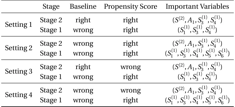
Table 4.6 Simulation settings in Section 6.2 . . . 98
Table 4.7 Simulation results for Setting 1 and 2 (%, standard deviations in paren-thesis) . . . 99
Table 4.8 Simulation results for Setting 3 and 4 (%, standard deviations in paren-thesis) . . . 100 Table 5.1 Rejection probabilities (%) of the sparse random projection-based test, dense
Table 5.2 Rejection probabilities (%) of the sparse random projection-based test, dense ran-dom projection-based test, penalized least square-based test, step-wise selection-based test and the supremum-type test selection-based on the desparsified Lasso estimator, with standard errors in parenthesis (%), under Scenarios 3 and 4 whereX0∼N(0,Ip).124
Table 6.1 Simulation results. . . 152
Table 6.2 P-values of each test statistic in all iterations. . . 154
Table 7.1 Simulation setting . . . 175
Table 7.2 ACP and AL of the CIs with standard errors in parenthesis . . . 176
Table 7.3 Simulation setting . . . 179
Table 7.4 ACP and AL of the CIs with standard errors in parenthesis . . . 180
LIST OF FIGURES
Figure 2.1 Plots ofβP (denoted by the snow symbol),βM (denoted by the circle symbol), andβg of the training (denoted by the square symbol) and testing groups (denoted by the plus symbol) for the second (left panel) and third (right panel) cases. . . 17 Figure 2.2 Plots ofβg (denoted by the square symbol), E?{1,2,3}(B)(denoted by
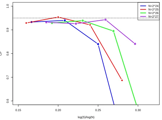
the snow symbol) and E?{1,2}(B)(denoted by the circle symbol) . . . 22 Figure 3.1 Coverage probability of 95% predictive interval with different choices
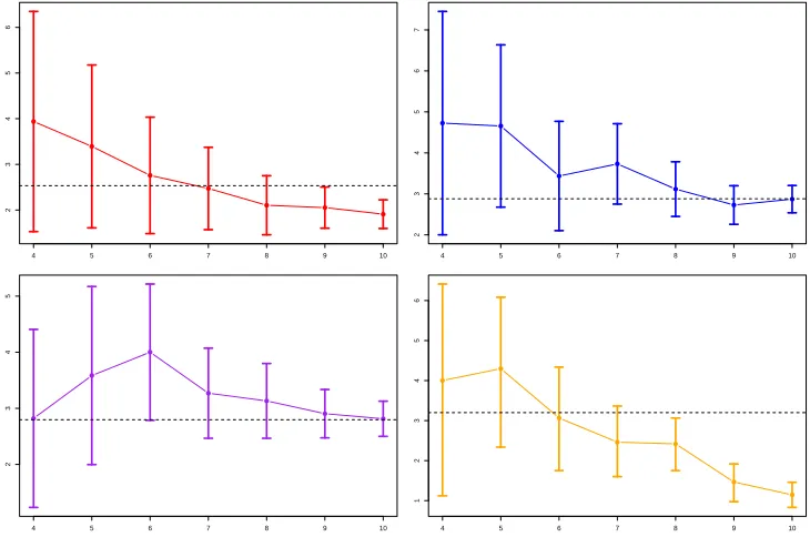
ofN andS, for the value search estimator . . . 48 Figure 3.2 95% confidence intervals ofθ0(1),θ0(2),θ0(3) andθ0(4) from top to
bot-tom and from left to right, against log(S)/log(2). Dash lines are the correspondingθ0(i)’s. . . 50 Figure 6.1 Plots of functionϕ2for Scenario 1 and Scenario 2, from left to right,
CHAPTER
1
INTRODUCTION
In precision medicine, individualizing the treatment decision rule can capture patients’ heterogeneous response towards treatment (Piquette-Miller and Grant 2007). In finance, individualizing the investment decision rule can improve individual’s financial well-being (Ding et al. 2019). In a ride-sharing company, individualizing the order dispatching strategy can increase its revenue and customer satisfaction (Xu et al. 2018).
In the literature, various methods have been proposed to estimating the OTR (or ODTR), including Q-learning (Watkins and Dayan 1992; Chakraborty et al. 2010; Song et al. 2015) and A-learning (Robins et al. 2000; Murphy 2003). Both Q-learning and A-learning rely on a backward induction algorithm to find the optimal dynamic treatment regime, however, Q-learning models the conditional mean of the outcome given predictors and treatment while A-learning directly models the contrast function that is sufficient for treatment decision. In particular, A-learning has the so-called doubly robust property, i.e. when either the baseline mean function or the propensity score model is correctly specified, the resulting A-learning estimating equation for the contrast function is consistent. Recently, Zhang et al. (2012, 2013) proposed to estimate the O(D)TR by directly maximizing the estimated expected outcome, i.e, the value function. Fan et al. (2017) introduced a type of concordance function for prescribing treatment and proposed a concordance-assisted learning for estimating the O(D)TR. Some other popular methods include outcome weighted learning (Zhao et al. 2012, 2015), tree-based methods (Laber and Zhao 2015; Zhu et al. 2017) and decision list-based methods (Zhang et al. 2015, 2018).
1.1
Motivation: the need for analyzing complex data
With the fast development of new technology, modern datasets often consist of massive observations, high-dimensional covariates and are characterized by some degree of het-erogeneity. In a ride-sharing company such as Didi Chuxing (one of the world’s leading ride-sharing platforms), its app generates more than 70TB of data every day. In a world of explosively large data, effective estimation procedures are needed to deal with the compu-tational challenge arisen from analysis of massive data.
Moreover, the OTRs may also vary for patients from different subpopulations. This is typically the case in meta analysis, where we combine the results of multiple studies conducted at different locations or times. One motivating example is from a multi-centre randomised controlled trial as studied in Tarrier et al. (2004). The goal is to examine the effectiveness of cognitive-behavioural therapy for patients with early schizophrenia. Pa-tients can be classified into three groups according to their treatment centres (Manchester, Liverpool and North Nottinghamshire). As we can see in Section 2.6.2, the group-wise OTRs can vary across different centres. Another example is from an observational study for inves-tigating the influence of early disease modifying antirheumatic drug (DMARD) treatment on patients with recent onset inflammatory polyarthritis (Farragher et al. 2010). According to patients’ enrollment time, they can be classified into three groups. As studied in Section 2.6.1, the group-wise OTRs can vary across different enrollment periods. The heterogeneity in OTRs may be explained by the differences in characteristics of treatment setting across subgroups. For instance, in the schizophrenia example, the strength of therapeutic alliance between therapist and patient, the adherence to treatment protocols and the quality of treatment provided can vary from one treatment centre to another (Dunn and Bentall 2007); in the inflammatory polyarthritis example, there are more use of hydroxychloroquine for the methotrexate combination strategy in recruitment time group 3 (1997-2000) than in group 1 (1990-1992) or group 2 (1993-1996) as hydroxychloroquine was increasingly used in the UK before anti-tumour necrosis factor therapy was introduced to treat rheumatoid arthritis in 2001. Moreover, these characteristics are often unobserved or partially observed, and they may explain the interaction between subgroups and OTRs.
These applications motivate us to develop statistical learning methods with complex datasets. Before presenting our methodologies, we introduce a causal framework (Rubin 2005) to formulate our problem. In Section 1.2, we introduce the model setup and formally define the OTR in a point treatment study. In Section 1.3, we focus on multiple time point studies and define the corresponding ODTR.
1.2
Point treatment study
outcomes, representing the response he/she would get if treated by treatment 0 and 1, respectively. In addition, define the potential outcome
Y0∗(d) =Y0∗(0){1−d(X0)}+Y0∗(1)d(X0),
representing the response a patient would have if treated according to a TRd. LetV(d) =
E{Y0∗(d)}be the value function under a TRd. An OTRdo p t is defined as the maximizer of
the expected potential outcomeV(d)among the set of all possible treatment regimes, i.e,
do p t ≡arg max d
V(d).
However, the OTR may not be unique. LetDo p t denote the set of all OTRs, i.e,
Do p t ={d0:V(d0) =max d V(d)}. Assume the following three assumptions hold.
(C1.) SUTVA:Y0= (1−A0)Y0∗(0) +A0Y0∗(1). (C2.) No unmeasured confounders:Y∗
0(0),Y0∗(1)⊥⊥A0|X0.
(C3.) Positivity:π(a,x)≥ε0,∀a ∈ {0, 1},x∈Xfor some constant 0< ε0<1, whereπ(a,x) =
P(A0=a|X0=x)denotes the propensity score function that characterizes the treatment assignment mechanism. We may sometimes use a shorthand and writeπ(1,x)asπ(x).
Define the contrast function
τ(x)≡h(1,x)−h(0,x),
whereh(a,x) =E(Y0|A0=a,X0=x), fora ∈ {0, 1}. We may sometimes writeh(0,x)ash(x). The following lemma relates OTR to the functionτ(·).
Lemma 1.2.1 LetX1={x∈X:τ(x)>0}andX2={x∈X:τ(x)<0}. Assume C1-C3 hold,
andE|τ(X0)|<∞. Then, for any d ∈ Do p t, we have
P(X0∈X1∩X2,d) =0 and P(X0∈X2∩X1,d) =0, (1.1)
whereX1,d ={x∈X:d(x) =1}andX2,d ={x∈X:d(x) =0}. Conversely, for any treatment
Lemma 1.2.1 implies thatdo p t,0∈ Do p t where
do p t,0(x) =I{τ(x)>0}, ∀x∈X, (1.2)
whereI(·)stands for the indicator function. The proof of Lemma 1.2.1 can be found in Shi
et al. (2019d).
The objective is to estimate an OTRdo p t∈ Do p tbased on the observed data{(Xi,Ai,Yi)}i that are assumed to be i.i.d copies of(X0,A0,Y0). In view of (1.2), one way to derive the OTR is to estimateτ(·). Q-learning and A-learning fall into this category. Denoted byτb(·)the estimated contrast function, the estimated OTR can is given byI{τb(·)>0}. Value-search methods, outcome weighted learning, concordance-assisted learning, tree-based methods and decision list-based methods, on the other hand, directly searchdo p t among a restricted class of TRs that maximizes some estimated value function.
1.3
Multiple time point study
Consider a multistage study where the treatment decisions are made at a finite number of time pointst1, . . . ,tK. The data for a subject can be summarized as
(X0(1),A0(1),X0(2),A0(2), . . . ,X0(K),A(0K),Y0),
whereY0denotes the outcome of interest,X( 1)
0 stands for the set of covariates obtained prior to the time pointt1,A(
1)
0 denotes the treatment received att1. Fork=2, . . . ,K,X( k)
0 denotes some additional covariates collected between time pointstk−1andtk, andA(
k)
0 denotes the treatment given attk. For simplicity, we assumeA(
1) 0 , . . . ,A
(K)
0 are all binary treatments. For
k=1, . . . ,K, let
¯
X0(k)= (X0(1), . . . ,X0(k))∈X¯(k) and A¯(0k)= (A(01), . . . ,A(0k))∈ {0, 1}k,
denote a patient’s covariates and treatment history. For anya1, . . . ,aK ∈ {0, 1}, denoted by ¯
ak = (a1, . . . ,ak)fork=1, . . . ,K. The set of all potential outcomes is given by
W= X0(2)∗(a1),X0(3)∗(a¯2), . . . ,X0(K)∗(a¯K−1),Y0∗(a¯K)
:∀a¯K ∈ {0, 1}K , (1.3)
points(t1, . . . ,tk−1)andY0∗(a¯K)denotes the potential outcome that would result assuming he/she receives treatments(a1, . . . ,aK).
A dynamic treatment regimed ={dk}Kk=1is a set of decision rules that treats a patient over time. Fork =1, . . . ,K,dk =dk(a¯k−1, ¯xk)corresponds to thek-th decision rule that takes as input a patient’s realized covariate and treatment history and outputs a treatment optionak ∈ {0, 1}. Let ¯dk ={dj}kj=1fork =1, . . . ,K −1, the potential outcome associated withd is given by
X0(2)∗(d1),X0(3)∗(d¯2), . . . ,X0(K)∗(d¯K−1),Y0∗(d)
,
whereX0(k)∗(d¯k−1)stands for the potential covariates of a patient betweentk−1andtk assum-ing he/she receives the treatments sequentially according to the decision rules(d1, . . . ,dk−1) andY∗
0(d)stands for the potential outcome assuming the treatments he/she receives are determined by the treatment regimed. An optimal dynamic treatment regimedo p t is defined to maximize the average potential outcome, i.e,
do p t =arg max d
EY0∗(d) =arg max
d
V(d).
For any ¯aK ∈ {0, 1}K and ¯xK ∈X¯(K), lethK(a¯K, ¯xK) =E(Y0|X¯( K)
0 =x¯K, ¯A( K)
0 =a¯K)and
τK(a¯K−1, ¯xK) = hK{(a¯K−1, 1), ¯xK} −hK{(a¯K−1, 0), ¯xK}. In addition, fork = K −1,· · ·, 2, we sequentially define
hk(a¯k, ¯xk) =E
arg max ak+1∈{0,1}
hk+1{(a¯k,ak+1), ¯X0(k+1)}
¯
X0(k)=x¯k, ¯A(k0)=a¯k
,
andτk(a¯k−1, ¯xk) =hk{(a¯k−1, 1), ¯xk} −hk{(a¯k−1, 0), ¯xk}, for any ¯ak∈ {0, 1}k and ¯xk∈X¯(k). For
k=1, let
h1(a1,x1) =E
arg max a2∈{0,1}
h2{(a1,a2),X¯0(2)}
X0(1)=x1,A(01)=a1
andτ1(x1) =h1(1,x1)−h1(0,x1)for anya1∈ {0, 1},x1∈X¯1. Define the propensity score functionπk(a¯k, ¯xk) =P(A(k0)=ak|X¯0(k)=x¯k, ¯A(k−
1)
0 =a¯k−1)fork=2, . . . ,K andπ1(a1,x1) =
P(A(01)=a1|X( 1)
0 =x1). Under the following three conditions, (MC1.)X0(k)=P
¯
ak−1∈{0,1}k−1X (k)∗
0 (a¯k−1)I(A¯(k− 1)
0 =a¯k−1)and
Y0=
P ¯
aK∈{0,1}K Y
∗
0(a¯K)I(A¯(K0 )=a¯K),∀k=2, . . . ,K and ¯aK ∈ {0, 1},
(MC3.)πk(a¯k, ¯xk)≥ε0,∀a¯k∈ {0, 1}k, ¯xk∈X¯k,k∈ {1, . . . ,K}, we can show
h(a¯K, ¯xK) =E{Y0∗(a¯K)|X¯0(K)∗(a¯K−1) =x¯K}, (1.4)
and for 2≤k≤K −1,
h(a¯k, ¯xk) =E[V0(k+1){a¯k, ¯X0(k+1)∗(a¯k)}|X¯0(k)∗(a¯k−1) =x¯k], (1.5)
and
h(a1,x1) =E[V0(2){a1, ¯X0(2)∗(a1)}|X0(1)=x1], (1.6)
where
V0(K)(a¯K−1, ¯xK) = max aK∈{0,1}
E{Y0∗(a¯K)|X¯0(K)∗(a¯K−1) =x¯K},
V0(k)(a¯k−1, ¯xk) = max ak∈{0,1}
E[V0(k+1){a¯k, ¯X0(k+1)∗(a¯k)}|X¯0(k)∗(a¯k−1) =x¯k], ¯
X0(k)∗(a¯k−1) ={X0(1),X0(2)∗(a1), . . . ,X0(k)∗(a¯k−1)}.
Here, Condition MC2 and MC3 automatically holds in sequentially randomized studies (Murphy 2005).
Define the set of dynamic treatment regimesDo p t such that anyd ={d
k}Kk=1∈ D o p t shall satisfy
dK(a¯k−1, ¯xk)∈arg max a∈{0,1}
aτk(a¯k−1, ¯xk),k=2, . . . ,K, (1.7) and d1(x1)∈arg max
a∈{0,1}
aτ1(x1),
for any ¯xK ∈X¯(K), . . . , ¯x2∈X¯(2),x1∈X¯(1) and ¯aK−1∈ {0, 1}K−1, . . . , ¯a2∈ {0, 1}2,a1∈ {0, 1}. By (1.4)-(1.6) and backward induction, we can show that
Do p t ⊆arg max d
EY0∗(d).
Notice that the argmax in (1.7) is not unique whenτk(a¯k−1, ¯xk) =0 orτ1(x1) =0. There-fore, the optimal dynamic treatment regime may not be unique. Given the observed data
Do p t.
1.4
Notations
In this section, we introduce some common notations used in this thesis. Throughout this thesis, we useC0and ¯C to denote some universal constants, whose values may change from place to place. For any arbitrary matrixΦ∈RM×M and any arbitrary vectorφ∈RM, the
superscriptΦ(j)is used to denote thejth column ofΦ,φ(j)thejth element ofφ. For subsets
J,J0⊂ {1, . . . ,M}, let|J|be the cardinality ofJ,Jc be the complement of J. We denote by
φJ the vector in
R|J|that has the same coordinates asφonJ, andΦJ the submatrix formed
by columns inJ,ΦJJ0the submatrix formed by rows inJ and columns inJ0. Letkφk
p denote the`p norm ofφandkΦkp denote the operator norm corresponding to thep-norm vector. We useIM to denote anM×M identity matrix.
For any two random variables Z1 andZ2,Z1 d
= Z2 meansZ1 andZ2 have the same distribution function. The notations→d and→P stand for convergence in distribution and convergence in probability, respectively. LetkZkψp be the Orlicz norm for any random variableZ, defined as
kZkψp ≡infu>0
Eexp
|Y|
u
p ≤2
,
for somep≥1. We useΦ(·)to denote the cumulative distribution function of a standard normal random variable. In addition,zα denotes theαth upper quantile of a standard normal distribution.
For any two positive sequences{an}and{bn},an bn means limnbn/an =0. The notationanbnmeans there exists some universal constantC0≥1 that satisfiesC0−1bn≤
an≤C0bn.
1.5
Outline
In Chapter 4, we propose a penalized A-learning method to estimate the ODTR with high-dimensional covariates. In Section 4.10, we also propose two doubly robust information criteria (concordance and value information criteria) for selecting the tuning parameters in penalized A-learning.
Chapter 5-7 are concerned with statistical inference regarding the O(D)TR. In Chapter 5, we propose to test if implementing the OTR is equivalent to the “one-size-fits-all" method. In Chapter 6, we further develop a test for assessing the incremental value of a set of new variables in treatment decision making conditional on an existing set of variables. In Chapter 7, we proposed to construct the confidence interval for the optimal value, based on subsample aggregating and refitted cross validation.
CHAPTER
2
MAXIMIN-PROJECTION LEARNING FOR
HETEROGENEOUS DATA
2.1
Introduction
Data from clinical trials and medical studies are often characterized by some degree of inhomogeneity. Optimal treatment regimes have been developed to account for patients’ heterogeneity in response to treatment. However, the OTRs may also vary for patients from different subpopulations. This is typically the case in meta analysis, where we combine the results of multiple studies conducted at different locations or times (see two real data examples in Section 2.6 for details).
different quality of treatment provided in the new treatment centre. Therefore, the true OTR for the group of new patients is not estimable at all based on the observed data, and any of the group-wise OTRs may not be the best choice. The challenge becomes how to derive a meaningful and reliable treatment regime that can take into account the heterogeneity in optimal treatment decision for different groups of patients. One simple approach is to pool the data of different groups together and obtain the “pooled" OTR based on the pooled data. Another method is to first obtain the OTR for each group, and then aggregate the group-wise OTRs in certain ways. Random effects meta-analysis (DerSimonian and Laird 1986) is commonly used to combine subject-specific studies. Using its multivariate extensions (see for example, Jackson et al. 2010; Chen et al. 2012), we can aggregate the groupwise OTRs based on random effects models. The resulting OTR is similar to the “pooled" OTR when we have large numbers of subgroup patients. These OTRs maybe reasonable choices when the OTRs for different groups do not vary much. However, when there is certain degree of heterogeneity in OTRs across different groups as demonstrated in the toy example given in the next section, these OTRs are uniformly worse than the proposed OTR for any of the groups. One possible reason is that these OTRs for different groups may assign the same patient to different treatments and thus their effects are averaged out when pooling the data from different groups.
Bühlmann and Meinshausen (2016) and Meinshausen and Bühlmann (2015) considered a maximin criteria which has a nice characterization in linear models and proposed to use maximin aggregation (magging) to obtain the maximin estimator. Their proposed estimator is shown to be more robust than the pooled estimator in linear regression. The key idea of the maximin criteria is to find an estimator that works the best under the worst-case scenario. In optimal treatment decision, the percentage of making the correct decision (PCD) and value function are two commonly used measures to evaluate the effectiveness of a treatment regime. A natural maximin criteria for optimal treatment decision is to find an OTR that maximizes the minimum PCD or the minimum value function of all groups. Such a maximin OTR is appealing due to its nice interpretation and robustness. However, it is hard to implement in practice due to the following reasons. First, the PCD of a treatment regime is generally not estimable from data since the true OTR is unknown. Second, the empirical estimator of the value function as studied in Zhang et al. (2012) is non-smooth and non-concave, thus the estimation of the associated maximin OTR is not feasible.
param-eters in the linear rule and the group-wise linear OTRs. We show that under certain model assumptions, the OTR obtained by MPL maximizes the minimum percentage of making the correct decision and value function of different groups, i.e. achieve the desired maximin properties. In addition, the corresponding estimation procedure can be represented as a linear programming problem with a quadratic constraint (Lee et al. 2016), which can be efficiently solved inO(G p2+p3)flops. HereG denotes the number of groups andp the dimension of baseline covariates. Consistency and the asymptotic distribution of the corresponding maximin-projection estimators are established. Such kind of asymptotic results are rarely studied in the literature. To derive such asymptotic properties, we establish a necessary and sufficient condition for the existence and uniqueness of the population maximin-projection parameters and obtain a closed-form expression for the resulting estimator.
The rest of the chapter is organized as follows. In Section 2.2, we introduce the model setup, and provide a heuristic comparison between the maximin OTR, the pooled OTR and the OTR based on random effects models with a toy example. In Section 2.3, we formally introduce the proposed maximin-projection learning including its statistical interpretation and geometrical characterization. Section 2.4 presents the estimating procedure of the maximin-projection estimator and the associated asymptotic properties. Simulation studies to evaluate the empirical performance of the proposed maximin OTR are conducted in Section 6.6. We apply our method to two real examples in Section 2.6. All the proofs and additional numerical studies can be found in Shi et al. (2018c).
2.2
Preliminaries and a toy example
2.2.1
Preliminaries
We consider a single stage study with two treatments. The setting considered in this chapter is slightly different from that in Section 1.2, since we need to take population heterogeneity into account. Specifically, we assume there areG groups of patients. Forg =1, . . . ,G, let
Y0,g,A0,g andX0,g denote the response, the (binary) treatment and the baseline covariates of patients in Groupg. In addition, letY∗
0,g(0)andY0,∗g(1)be the corresponding potential outcomes and definehg(a,x) =E{Y0,∗g(a)|X0,g =x}fora ∈ {0, 1}. We may sometimes use a shorthand and writehg(0,x)ashg(x). For any treatment regimed(·)that maps the covariate space to{0, 1}, defineY∗
For simplicity, assume the contrast function is linear, i.e,
hg(1,x)−hg(0,x) =βgTx+cg, ∀x,
for someβg ∈Rpandcg∈R. Suppose SUTVA, no unmeasured confounders and the positivy assumption hold. It follows that
E(Y0,g|A0,g=1,X0,g=x)−E(Y0,g|A0,g =1,X0,g =x) =βgTx+cg, (2.1)
E(Y0,g|A0,g=1,X0,g=x) =hg(x), ∀x. (2.2) Without loss of generality, we further assume all covariates X0,gs are standardized to have zero mean and identity covariance matrix. Otherwise, we consider variable trans-formationX∗
0,g =Σ
−1/2
g (X0,g −µg),β∗g =Σ 1/2
g βg,cg∗ =cg+µgTβg whereµg =E(X0,g)and
Σg=COV(X0,g). Then Model (2.1) can be represented as
E(Y0,g|A0,g=1,X0,∗g=x)−E(Y0,g|A0,g =1,X0,∗g =x) =x Tβ∗
g+c
∗
g,
E(Y0,g|A0,g=0,X0,∗g=x) =hg∗(x), ∀x, for some functionh∗
g.
The parametercg stands for the marginal treatment effects (average causal effects) after adjusting covariates. Mathematically, we have
cg=E(βTgX0,g+cg) =E[E{Y0,∗g(1)|X0,g} −E{Y0,∗g(0)|X0,g}].
Whencg>0, treatment 1 is generally better for patients in Groupg. The vectorβgdescribes individualized treatment effects. For patients in Groupg with covariatesx, the largerβT
gx, the more benefits he or she receives if assigned to treatment 1.
Defineπg(a,x) =P(A0,g=a|X0,g =x)fora ∈ {0, 1}as the propensity score in Groupg. We will sometimes writeπg(1,·)asπg(·). Model (2.1) allowshg andπg to vary across groups, which we refer to baseline effect heterogeneity and treatment assignment heterogeneity respectively. These sources of heterogeneity are not related to treatment decisions since they do not appear in the contrast function. The following sources of groupwise heterogene-ity will affect decision making: the marginal treatment effectscg and the individualized treatment effectsβg. In this chapter, we mainly focus on heterogeneity caused by different
To introduce the pooled and the maximin optimal treatment regime, we need some optimality criterion. Here, we consider the difference of patient’s mean response (value function) between a regimed(x) =I(βTx>−c)andd
0(x) =0, which assigns all patients to treatment 0. Specifically, the difference of value functions is defined as
VDg(β,c) =E{Y0,∗g(d)} −E{Y
∗
0,g(d0)}=E{(X0,Tgβg+c0)I(X0,Tgβ>−c)}.
In this section, for illustrative purposes only, we consider a special case withc0=c =0. A general discussion will be given in the next section. When the distributions ofX0,gs are the same across groups, we can represent VDg(β, 0)as
VD(β,βg) =E{(X0,Tgβg)I(X0,Tgβ>0)}.
We assume the same number of patients across all groups. Then, the pooled optimal treatment regime is defined asdPo p t,0(x) =I(xTβP >0)where
βP =arg max
kβk2=1 1
G
G X g=1
VD(β,βg), (2.3)
and the maximin optimal treatment regime is defined asdMo p t,0(x) =I(xTβM >0)where
βM =arg max
kβk2=1
min
g∈{1,...,G}VD(β,βg). (2.4)
We add the L2 constraint onβ to makeβP andβM identifiable. Therefore, the pooled optimal treatment regime aims to maximize the average value difference while the maximin optimal treatment regime aims to maximize the minimum value difference inG groups, i.e. maximize the reward of the worst-case scenario.
The random effects meta-analyses assume the following model forβg’s:
βg =β0+εg,
whereεg’s are independent and satisfyE(εg) =0,COV(εg) =Ω0for allg. For any subgroup estimatorsβb1, . . . ,βbG withCOV(βbg) =Ωg, the aggregated estimator is given by
b
βR =
G X g=1
(Ωbg+Ωb0)−1
−1 G X g=1
(Ωbg+Ωb0)−1βbg
whereΩbg’s andΩb0denote some estimators forΩg’s andΩ0. Given sufficiently many obser-vations, we havekβbg−βgk2
P
→0 andkΩbgk2 P
→0. As a result, we have
b
βR P→
G X g=1
(Ωb0)−1
−1 G X g=1
(Ωb0)−1βg
= 1
G
X g
βg ≡βR. (2.5)
The corresponding optimal treatment regime is defined asdRo p t,0(x) =I(xTβR>0).
More generally, we can treat the parametersβg in the group-specific contrast function as a multivariate random variable and assume that the parametersβg’s of training groups are generated according to some distributionF, either continuous or discrete, and letH
denote the support ofF. Then, we defineβR,βP andβM as
βR = Etrain(b),
βP = arg max
kβk2=1
Etrain{VD(β,b)},
βM = arg max
kβk2=1 min
b∈H VD(β,b),
where the expectationEtrainis taken with respect toF. Definitions in (2.3), (2.4) and (2.5) correspond to the special case whereF only takes values in{β1, . . . ,βG}with an equal probability. Our objective is to minimizeEtest{VD(β)}, whereEtestis taken with respect to
G, the distribution ofβg for future groups of patients.
2.2.2
A toy example
Recall thatp is the dimension ofX0,g. For illustration, we takep =2, and assume that pa-tients’ baseline covariates are generated independently from a standard normal distribution. Sincekβk2=1, after some calculation, we have
VD(β,βg) = E{X0,TgβgI(X0,Tgβ>0)}=E{(X0,Tgβg−βgTβX0,Tgβ+βgTβX0,Tgβ)I(X0,Tgβ>0)} = βTgβE
¦
X0,TgβI(X0,Tgβ>0)
©
=βgTβp1
2π.
βTgβX0,TgβandX0,Tgβ. Hence, we obtain
βP =arg max
kβk2=1 1
G
G X
g=1
βTβg = P
gβg
kP gβgk2
,
βM =arg max
kβk2=1
min g∈{1,...,G}β
T
βg. (2.6)
Therefore, βP is proportional to βR which equals a simple average of all subgroup parameters, whileβM maximizes its minimum inner product across differentβ
g’s. When allβg’s have the sameL2norm,βM becomes
βM =arg max
kβk2=1
min g∈{1,...,G}
βTβ g
kβgk2, (2.7)
or equivalently
βM =arg min
kβk2=1
max
g∈{1,...,G}∠(β,βg), (2.8)
where∠(a,b) =arccos(aTb)stands for the angle between two vectors. The equivalence between (2.7) and (2.8) is due to the monotonicity of the arccos function. In (2.7) or (2.8),βM is defined to maximize (minimize) the minimum correlation (maximum angle) between all subgroup coefficients. Such formulation is referred to as the maximin correlation approach in the classification literature (c.f, Avi-Itzhak et al. 1995; Lee et al. 2016). In general, we weight the correlationβTβg/kβgk2by theL2norm ofβg. TheβM defined in (2.6) is more informative since it not only takes the heterogeneity due to different directionsβg/kβgk2 into consideration, but different magnitudeskβgk2as well.
SinceβP is proportional toβR, the VD underdo p t,0
P is the same asd o p t,0
R . Therefore, in the following, we focus on comparingβP withβM. We setG =4 and assumekβ
gk2=1,
g =1, 2, 3, 4. Sincep =2, we represent eachβg asβg ={cos(ψg), sin(ψg)}T withψ
g ∈[0,π). The parameterψg is the angle betweenβg and thex-axis in a 2-dimensional coordinate system. In this special case,βM lies on the bisector of the largest angles formed by allβ
g’s and it can be shown thatβM ={cos(ψM), sin(ψM)}T where
ψM =1
2 ψ(1)+ψ(4)
,
ψ(1)andψ(4)denote the smallest and largest angles ofψg’s. Similarly defineβP ={cos(ψP), sin(ψP)}T. We setψ
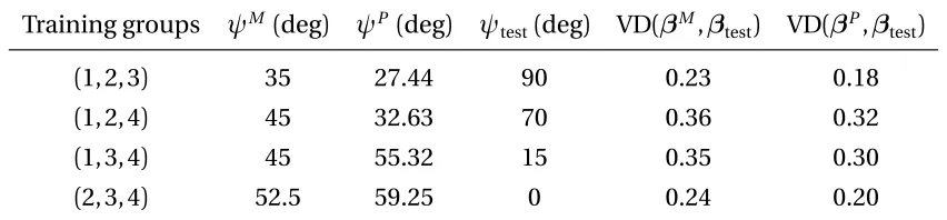
90°. Consider the following leave-one-group-out cross validation procedure. For theith round, we choose theith group as the testing group, and obtainβP andβM based on the remaining 3 groups. Then we evaluate the value difference of the pooled and maximin OTRs based on theith group. In other words, we setF to be a discrete distribution that takes value on{β1, . . . ,β4}/{βi}with equal probability, andG a degenerate distribution that concentrates onβi. Table 2.1 summarizes the results.
Table 2.1: Different combinations of training groups and the correspondingψP,ψM, and their value differences on the testing group
Training groups ψM (deg) ψP (deg) ψ
test(deg) VD(βM,βtest) VD(βP,βtest)
(1, 2, 3) 35 27.44 90 0.23 0.18
(1, 2, 4) 45 32.63 70 0.36 0.32
(1, 3, 4) 45 55.32 15 0.35 0.30
(2, 3, 4) 52.5 59.25 0 0.24 0.20
From Table 2.1, we can see that for all four cases, the value differences of the maximin optimal treatment regime are uniformly larger than those of the pooled optimal treatment regime on the testing groups. To illustrate the idea graphically, we plotβP (denoted by the snow symbol),βM (denoted by the circle symbol), andβ
g of the training (denoted by the square symbol) and testing (denoted by the plus symbol) groups for the second and third cases in Figure 6.1, where the left panel is for the second case and the right one is for the third case. For both cases,βM is closer toβ
g of the testing groups, whileβP is pulled towards the area where mostβg’s of the training groups locate due to the averaging effect.
-1 -0.5 0 0.5 1
x -1
-0.8 -0.6 -0.4 -0.2 0 0.2 0.4 0.6 0.8 1
y
-1 -0.5 0 0.5 1
x -1
-0.8 -0.6 -0.4 -0.2 0 0.2 0.4 0.6 0.8 1
y
2.3
Maximin-projection learning
We now formally introduce our maximin projection treatment regime. Based on model (2.1) and the common marginal treatment effect assumption, the optimal treatment regime for thegth subgroup isdo p t,0
g (x) =I(x Tβ
g >−c0). Here, our goal is to find a single treat-ment regimedMo p t,0(x) =I(xTβM >−cM)withkβMk2=1 that performs uniformly well for heterogeneous data. Motivated by the toy example in the previous section, our proposed maximin-projection learning is aim to find
βM =arg max β:kβk2=1
min g∈{1,...,G}β
T
βg.
2.3.1
Statistical interpretation
In this subsection, we show that the maximin projection, represented byβM, has two nice statistical interpretations in terms of maximizing the minimum PCD and value difference (VD). Specifically, in groupg, the PCD of a treatment regimed(x) =I(xTβ>−c)is defined as
PCDg(β,c) =1−E{|I(X0,Tgβ>−c)−I(X0,Tgβg >−c0)|},
and the VD is defined as
VDg(β,c) =E[Y0,∗g{I(X T
0,gβ>−c)}]−E{Y
∗
0,g(0)}=E ¦
(X0,Tgβg+c0)I(X0,Tgβ>−c) ©
.
Here, the larger PCD and VD values, the better the treatment regimed(x)approximates the groupwise optimal treatment regimedo p t,0
g (x).
Based on the defined PCD and VD, for any fixed constantc, we consider the following maximin treatment regimes:d1(x) =I(xTβ(M1)>−c)where
β(M1)=arg max β:kβk2=1
min
g∈{1,...,G}PCDg(β,c), (2.9)
andd2(x) =I(xTβ(M2)>−c)where
β(M2)=arg max β:kβk2=1
min
g∈{1,...,G}VDg(β,c). (2.10)
The two maximin treatment regimes, defined byβM
statistical interpretations. However, we note that the definition ofβM(1)involves unknown parameters. The empirical estimators of VD are of non-smooth and non-concave functional forms of the corresponding estimators. Therefore, their estimations are not feasible and they may not be practically useful.
It is worth noting thatβM
(1)would be meaningless when not allkβgk2’s are the same. This is because PCD only measures the similarity between the overall and groupwise optimal treatment decisions, but does not account for the magnitude of groupwise contrast function. Whenkβgk2’s are not the same, theL2norm of groupwise contrast function{E(X0,Tgβg+
c0)2}1/2 would be different. This implies that PCDs are not comparable across different groups. In comparison, VD is a better criterion since it takes both the sign and magnitude of contrast function into consideration. Below, under some conditions, we establish the equivalence between these two maximin treatment regimes and our proposed maximin-projection treatment regime.
Theorem 2.3.1 (Equivalence ofβM andβ(M1)) Assume thatX0,g’s are i.i.d. spherically
dis-tributed, and allkβgk2’s are the same. Then, for any fixed c ,
βM =arg max
kβk2=1
min
g∈{1,...,G}PCDg(β,c).
Theorem 2.3.2 (Equivalence ofβM andβM
(2)) AssumeX0,g’s are i.i.d. spherically distributed.
Then, for any fixed c ,
βM =arg max
kβk2=1
min
g∈{1,...,G}VDg(β,c).
Theorems 2.3.1 and 2.3.2 requireX0,g to have a spherical distribution which requires
X0,g d
=U X0,g for any orthogonalp×p matrixU. This includes a rich class of symmetric multivariate distributions (see Fang et al. 1990).
The definition ofβM has nice statistical interpretations. However, it has two drawbacks. First, whenF0≡maxkβk2=1mingβTβg <0, the uniqueness ofβM is not guaranteed. This may cause identifiability issues when we establish properties of the corresponding esti-mators. In addition, the optimization problem in (2.6) is not concave. This can make the implementation of the estimating procedure infeasible.
To address these concerns, we define
βM(0)=arg max
kβk2≤1
min g∈{1,...,G}β
Tβ
Compared toβM, it replaces the feasible setkβk2=1 with a closed convex setkβk2≤1. Lemma 2.3.1 below states thatβ(M0)is well defined, whenF06=0. Moreover, the optimization problem (2.11) is concave, which can be easily implemented.
Lemma 2.3.1 The maximin-projection estimatorβM(0)always exists. Moreover, when F06=0,
βM(0)is unique.
The existence ofβM
(0)is guaranteed by the continuity of the objective functionF(β) = ming∈{1,...,G}βTβg, boundedness and closeness of the feasible setβ:kβk2≤1. Its uniqueness is a byproduct of lemma 2.3.3, which is stated in the next subsection. WhenF0=0,β(M0) is not unique and the set of solutions is given by
{aβ:a ∈[0, 1],kβk2=1, max
kβk2=1g∈{min1,...,G}β
T
βg =0}.
The problem of estimatingβM
(0)then becomes non-regular and all the large sample theories about the maximin estimator fail (see Section 2.4).
DefineG0=maxkβk2≤1mingβ Tβ
g. It is obvious thatG0 ≥0. In addition,G0>0 if and only ifF0>0. WhenG0=0, we can setβ(M0)=0, which leads to a trivial regime by assigning the same treatment to all patients. From now on, we focus on the situation whenG0>0. In this case, we haveβM =βM
(0). Define
c(M0) =c0/G0.
Note thatcM
(0) andc0are sign equivalent. Our maximin-projection OTR is given by
dMo p t,0(x) =I(x T
βM(0)>−c(M0)).
Theorem 2.3.3 Under conditions of theorem 2.3.1, if G0>0, we have
c(M0) =arg max c
min
g∈{1,...,G}PCDg(β
M (0),c).
Theorem 2.3.4 Under conditions of theorem 2.3.2, if G0>0, we have
c(M0) =arg max c
min
g∈{1,...,G}VDg(β
M (0),c).
groups.
2.3.2
Geometrical characterization
In this subsection we give a geometrical view ofβM(0)whenG0>0. Findings in this subsection are similar in rationale with the results in Avi-Itzhak et al. (1995). However, we generalize their results by getting rid of the unitL2-norm conditionkβgk2=1 and allowing the set of vectors{β1, . . . ,βG}to be linear dependent, which is the case whenp≥G.
We first introduce some notation. For an arbitraryp×G matrixΨand a setK ⊆ {1, . . . ,G}, letΨK denote the submatrice ofΨformed by columns inK. Define the equicorrelated points set
EK(Ψ) =
t∈Rp|tTΨj =tTΨi,∀i,j ∈K ,
and the optimal equicorrelated point
E?K(Ψ) =arg max t∈EK(Ψ)
ktk2=1
tTΨi,∀i ∈K ,
whereΨi refers to theith column vector of matrixΨ. When|K|=1 andΨK =ψ, E?K(Ψ) =
ψ/kψk2. Readers can refer to Shi et al. (2018c) for a detailed discussion on the equicorrelated points set and the optimal equicorrelated point.
For any matrixΩ, LetΩ+denote the Moore-Penrose matrix inverse ofΩandC(Ω)the column space ofΩ. Letedenote a vector of ones. We have the following result.
Lemma 2.3.2 For anyΨ and K ⊆ {1, . . . ,n}, whene∈C(ΨT
K), the optimal equicorrelated
point ofΨK exists and is unique. Moreover, it takes the form
E?K(Ψ) ={eT(ΨTKΨK)+e}−1/2ΨK(ΨTKΨK)+e. (2.12)
Define matrixB= (β1,β2, . . . ,βG)whosegth column is the subgroup parameterβg.
Lemma 2.3.3 Assume G0>0. Then there exists a unique nonempty set K0⊆ {1, . . . ,G}such
thatβM
(0)=E?K0(B)andming∈K0cβ M (0) T
βg>G0, where K0c={1, . . . ,G} −K0. Moreover, if the set
of vectorsβg,g ∈K0are linearly independent, then a necessary and sufficient condition for
βM
(0)=E?K0(B)is that each element in the vector(B
T K0BK0)
1.5 -0.4
-0.2 0
1 1
0.2 0.4
z
0.6
x 0.8
1
0.5
y
0.5 0
-0.5 0
-1
Figure 2.2: Plots ofβg(denoted by the square symbol), E?{1,2,3}(B)(denoted by the snow symbol) and E?{1,2}(B)(denoted by the circle symbol)
We denoteK0as the maximin optimal equicorrelated points set whenG0>0. In lemma 2.3.2, the conditione∈C(ΨTK)automatically holds whenΨTK has full row rank. In lemma 2.3.3, we assume the set of vectorsβg,g ∈K0are linearly independent. This implies the matrixBT
K0 has full row rank. As a result, we havee∈C(B T K0). In lemma 2.3.3, the non-negativity of(BT
K0BK0)
−1eis sufficient and necessary forβM (0)= EK0(B). Together with lemma 2.3.2, lemma 2.3.3 implies thatβ
M
(0) is uniquely defined by
β(M0)=E?K0(B) ={eT(BTK0BK0)
−1e
}−1/2BK0(B T K0BK0)
−1e.
This implies E?K
0(B)is proportional toBK0(B T K0BK0)
−1eand can be represented as a linear combination of the column vectors inBK0. Geometrically, the non-negativity of(BT
K0BK0)−1e requires E?K0(B)to lie in the convex cone ofβg,g ∈K0, i.e,{
P
g∈K0agβg :ag ≥0,∀g ∈K0}. To better understand lemma 2.3.3, in Figure 2.2, we takes=3,G =3 andB= (β1,β2,β3) whereβ1= (1, 1, 0),β2= (1,−1, 0)andβ3= (1.2, 0, 0.5). Both E?{1,2,3}(B)and E?{1,2}(B)satisfy the necessary conditions of lemma 2.3.3. While E?{1,2}(B)lies in the convex cone ofβ1and
β2, E?{1,2,3}(B)appears outside the convex cone ofβ1,β2andβ3. Therefore, E?{1,2}(B) satis-fies the sufficient conditions of lemma 2.3.3 and E?{1,2,3}(B)does not. As a result, we have
βM
2.4
Estimation procedure
The data are summarized as(Yj,g,Aj,g,Xj,g), forg =1, . . . ,G, j =1, . . . ,mg, wheremg is the number of patients in Groupg. We assume that the data are independent acrossg =1, . . . ,G
and j =1, . . . ,mg. Based on the data, parametersβ1, . . . ,βG andc0in model (2.1) can be estimated with existing methods. In this chapter, we implement with the popular Q-learning and A-learning and give a brief discussion on estimating these parameters in Section 2.4.2. Letβb1, . . . ,βbG andcb0be the corresponding estimators. We propose to estimateβ(M0)by solving the following optimization problem:
b
βM =arg max β:kβk2≤1
min g∈{1,...,G}β
T b
βg. (2.13)
Note that the objective function mingβTβbg is concave inβand the regionkβk2≤1 is convex. Therefore, (2.13) is a tractable convex optimization problem. It can be further casted as a quadratic constraint linear programming (QCLP) problem, specifically,βbM is equivalent to the solution of
maximize t ∈R
subject to βTβbg ≥t,g =1, . . . ,G
βTβ≤1.
The above optimization problem can be efficiently computed using existing softwares. DefinecbM =
b
c0/GÒ0, whereGÒ0=mingβbgTβbM.
Given a group of future patients, denoted by{Xj,G+1}n
j=1their baseline covariates. We calculateµbG+1=Pn
j=1Xj,G+1/n andΣbG+1= Pn
j=1(Xj,G+1−µbG+1)(Xj,G+1−µbG+1)
T/(n−1). The recommend treatment for the jth patient is given by
I{(Xj,G+1−µbG+1) T
b
ΣG−1+/12βbM >−cbM}.
2.4.1
Statistical properties
In this subsection we investigate the asymptotic properties of the maximin-projection estimatorβbM obtained by solving the optimization problem (2.13). We first study the consistency of the estimator by assuming the following two conditions.
(S2.) Assume thatF06=0. WhenF0>0, assume that the column vectors inBK0 are linearly independent and all elements in the vector(BKT
0BK0)
−1eare nonzero, where K
0 is the maximin optimal equicorrelated points set as defined previously.
Condition S1 requires each subgroup estimator to be consistent. The conditionF06=0 in S2 ensures the existence and uniqueness ofβM
(0). Apparently,βM(0)is not stable whenF0 approaches to 0, since itsL2norm will change from 1 to 0. To ensure the stability ofβ(M0) in the sense that it will not deviate too much when there are minor changes in the set of vectorsβ1, . . . ,βG, we would expect
k(B˜K0T B˜K0)
+−(BT K0BK0)
+k
2→0, (2.14)
as ˜BK0 → BK0, where ˜B = (β˜1, . . . , ˜βG)represents the coefficient matrix with some dis-turbance. A sufficient condition to establish (2.14) is thatBK0 is of full column rank, as assumed in Condition S2. Lemma 2.3.2 suggestsβM
(0)can be represented asω0TBK0, for some weight vectorω0proportional to(BK0T BK0)
−1e. Condition S2 further assumes the weights are nonzero. Such a condition guarantees that for any coefficient matrix ˜B→B,K0is the optimal equicorrelated points set of ˜Bas well.
Theorem 2.4.1 (Consistency) DefineBÒ= (βb1, . . . ,βbG). Assume Conditions S1 and S2 are
satisfied. Then with probability tending to1, the estimatorβbM is equal to
¨
{eT(BÒTK 0BÒK0)
−1e}−1/2 Ò
BK0(BÒKT 0BÒK0)
−1e if F 0>0,
0 if F0<0.
In addition, assume there exist some r(1)
n ,r( 2)
n →0such thatmaxg∈K0kβbg−βgk2=Op(rn(1))and b
c0=c0+Op(rn(2)). When F0>0, we havekβbM −βM(0)k2=Op(rn(1)),cbM =c(M0) +Op(rn(1)+rn(2)). Theorem 2.4.1 implies that(βbM,cbM)is consistent as long as each subgroup estimator is consistent. The first part of the theorem follows as a consequence of lemma 2.3.3.
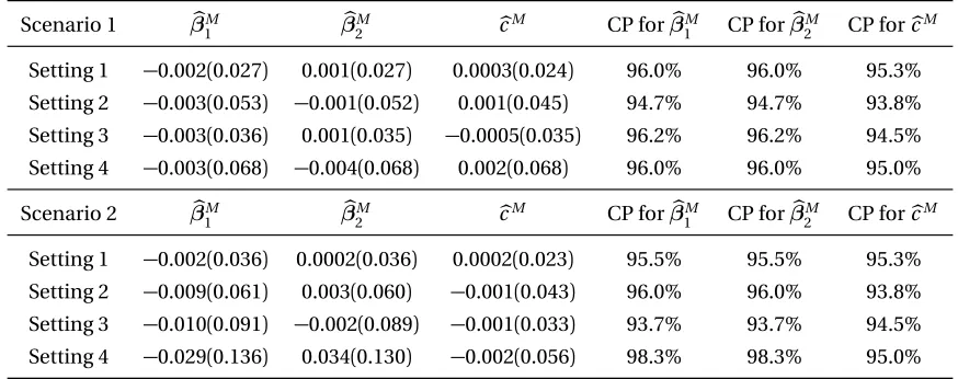
Next, we study the asymptotic normality of the estimator. For notational simplicity, we assumem1=· · ·=mG =m and posit the following condition.
(S3.) Assume that for allg ∈K0,
p
m(βbg−βg)andpm(cb0−c0)are jointly asymptotically normal with mean zero.
Theorem 2.4.2 (Asymptotic normality) Assume that Conditions S1–S3 hold, and that F0>