DOI: 10.1534/genetics.106.066530
Evolutionary Framework for Protein Sequence Evolution
and Gene Pleiotropy
Xun Gu
1Department of Genetics, Development and Cell Biology, Center for Bioinformatics and Biological Statistics, Iowa State University, Ames, IA 50011
Manuscript received October 5, 2006 Accepted for publication January 8, 2007
ABSTRACT
In this article, we develop an evolutionary model for protein sequence evolution. Gene pleiotropy is characterized byKdistinct but correlated components (molecular phenotypes) that affect the organismal fitness. TheseKmolecular phenotypes are under stabilizing selection with microadaptation (SM) due to random optima shifts, the SM model. Random coding mutations generate a correlated distribution of Kmolecular phenotypes. Under this SM model, we further develop a statistical method to estimate the ‘‘effective’’ number of molecular phenotypes (Ke) of the gene. Therefore, for the first time we can empirically
evaluate gene pleiotropy from the protein sequence analysis. Case studies of vertebrate proteins indicate that Keis typically6–9. We demonstrate that the newly developed SM model of protein evolution may provide a
basis for exploring genomic evolution and correlations.
A
LTHOUGH the wide availability of high-throughput data has greatly facilitated the study of evolutionary genomics, the foundation of molecular evolution has been relatively ‘‘static’’ (Kimura 1983). Basically, theevolutionary fate of a mutant is largely determined by the prespecified fitness value (the coefficient of selection) and the effective population size. Although this classical treatment has successfully removed the complexity of genotype–phenotype association, problems may appear when the association itself has been one of the research highlights. The recent debate about genomic correla-tions among evolutionary rate, interaction, expression, and dispensability has indicated the limitation of current evolutionary models (reviewed in Palet al.2006).
Alter-natively, researchers have to use the partial-correlation or principle-component methods to analyze major deter-minants governing protein evolution (e.g., Drummond et al.2005; Wallet al. 2005; Wolfet al. 2006), because
these approaches are not model dependent.
It is desirable to develop a novel framework that can provide an integrated view of protein evolution, but an unsolved key problem is how to deal with the sophisticated relationship between protein sequence and organismal fitness. We recognized that the substantial genotype– phenotype literature can be used to address this issue (e.g., Fisher1930; Lande1980; G. Wagner1989; Waxman
and Peck1998; A. Wagner2000; Poonand Otto2000;
Zhangand Hill2003). As mutations are raw materials
for evolution, the distribution of effects of mutations,
f(s), has been a central issue in the genotype–phenotype study (Lynchet al. 1999; Bataillon2000; Shawet al.
2002). Under Fisher’s geometric model (e.g., Fisher
1930; Hartland Taubes1998; Poonand Otto2000)
or multivariate model (e.g., Lande 1980; Welch and
Waxman2003; Martinand Lenormand2006),f(s) can
be predicted on the basis of selective and mutational assumptions. The dimensionality in each framework has been interpreted as the number of loci affecting a quan-titative trait (reviewed in Kingsolveret al. 2001), or the
number of affected phenotypic traits of a mutation, esti-mated from mutational-accumulation experiments (re-viewed in Elenaand Lenski2003). On the other hand,
anad hocgamma distribution forf(s) was introduced in the early days of the neutral theory of molecular evolution (Ohta1973, 1977; Kimura1983), which has been found
useful to estimate the proportion of neutral or deleteri-ous mutations (e.g., Nielsenand Yang2003; Piganeau
and Eyre-Walker2003; Eyre-Walkeret al. 2006).
Here we extend our recent work (Gu 2006). The
principle behind our present work in modeling protein sequence evolution is as follows: First, multifunctionality of a gene (pleiotropy) is characterized by K distinct components in the fitness (calledmolecular phenotypes). Second, these K molecular phenotypes are under sta-bilizing selection (Fisher 1930; Waxman and Peck
1998) with microadaptations due to random shifts of the fitness optimum (Gillespie1991). Third, random
mutations in the coding region of the gene generate a mutational distribution for K molecular phenotypes. Correlated structures among Kmolecular phenotypes are taken into account at both selectional and muta-tional levels. More importantly, we develop a statistical 1Address for correspondence:Department of Genetics, Developmental and
Cell Biology, 536 Science II Hall, Iowa State University, Ames, IA 50011. E-mail: [email protected]
method to estimate the ‘‘effective’’ number of molecular phenotypes (Ke) of the gene. Case studies of vertebrate proteins demonstrate that for the first time we can em-pirically evaluate gene pleiotropy only from phyloge-netic sequence analysis.
THE MODEL
Molecular phenotypes and gene pleiotropy: Pleiot-ropy of a gene (protein) function can be modeled by mul-tiple (K) molecular phenotypes, denoted by (y1,. . .,yK).
Each molecular phenotype yi represents a nontrivial
component of genetic variation, contrasting with or-ganismal fitness as a result of a specific (yet unknown) biological process (Figure 1). At one extreme, molecular phenotypes could correspond to subcomponents of protein function, regardless of the biological processes. At another extreme, molecular phenotypes could be determined mainly by distinct physiological processes. Since these underlying biological processes are usually intractable, the concept of molecular phenotypes based on fitness effects avoids this difficulty.
Following the widely used procedure (e.g., Lande
1980; Turelli1985; Waxmanand Peck 1998), we
as-sume that the fitness function of molecular phenotypes
y¼(y1,. . .,yK)9is Gaussian-like;i.e.,
wðyÞ ¼exp ðymÞ9S
1
w ðymÞ
2
; ð1Þ
wheremis the optimum of the fitness function, andSwis
a (positive definite) symmetric matrix characterizing correlated stabilizing selection onKmolecular pheno-types. The ith diagonal element s2
w;i measures the
strength of stabilizing selection on the ith molecular phenotype, while the ijth nondiagonal element sw,ij
measures the correlated stabilizing selection onyiandyj.
Lety0be the population mean of molecular pheno-types of a gene, which may not necessarily be at the op-timum (m). By definition (Fisher1930), the coefficient
of selection for the molecular phenotypeyis given by
rðyjy0;mÞ ¼wðyÞ=wðy0Þ 1: ð2Þ
Classical stabilizing selection (Turelli 1985; Waxman
and Peck1998) assumes that the population mean is
al-ways at the fitness optimum,i.e.,y0¼m, leading to purify-ing selection; that is,r(yjy0¼m)#0 always holds.
Next, we consider the effects of mutations on molec-ular phenotypes. A random mutation in the coding re-gion of a gene may affect molecular phenotypes in a correlated fashion (Figure 1). Such a pleiotropic muta-tional effect can be described by a multivariate normal distribution
pðyÞ ¼Nðy;ym;SmÞ; ð3Þ
where ym is the mean mutational effect on molecular phenotypes, and the covariance matrixSmmeasures the correlated mutational effects. The coefficient of selec-tionr(yjy0,m) and the distribution of mutational effects p(y) provide a connection between organismal fitness and protein sequence evolution through molecular pheno-typesy(Figure 1). Below we discuss the classical stabilizing selection model and the newly developed stabilizing se-lection with microadaptation (SM) model. See Figure 2 for illustration.
Stabilizing selection model:Under the classical stabi-lizing model, the population mean of molecular pheno-types (y0) is always fixed at the optimum (m). Without loss of generality, we assume thaty0¼m¼0. From Equation 2 one can show that r0ðyÞ ¼rðyjy0¼m¼0Þ y9S1w
y=2,0, reflecting the stabilizing (purifying) selection against deleterious mutations, which necessarily results in a deviation from the optimum. A consequence of this model is that sequence evolution is dominated by the fixation of very slightly deleterious mutations (Ohta
1973; Kimura1979, 1983).
For mathematical convenience, we assume that the mutational distribution,p(y) in Equation 3, is centered at the population mean, namely, ym¼y0¼ 0. In the following we consider mainly the selection intensityS(y)
¼4Ner0(y) ¼ 2Ne(y9S 1
w y), whereNeis the effective population size. Given Equation 3 ofp(y), the distribu-tion ofS,f(S), can be uniquely determined by the prob-ability theory (see theappendix). Although the analytical
form off(S) is available only for a few special cases, the moments ofScan be obtained readily. For instance, the mean ofScan be computed by
S¼ 2Ne ð
y9Sw1ypðyÞdy; ð4Þ
which is always negative.
Stabilizing selection with microadaptation model:
Consider the case when the fitness optimum (m) of a
Figure1.—Schematic presentation for the concept of
gene is no longer fixed during the evolution. Rather,m can be shifted either by environmental changes or by internal physiological perturbations. Each shift ofm re-sults in a microadaptation toward a new fitness optimum (Gillespie1991). Since the direction and strength of the m-shift are unobservable, we treatmas a (K-dimensional) random variable. Similar to the above, we assume that the population mean and the mutation mean satisfy
y0¼ym¼0. Then, under the SM model, the coefficient of correlation defined by Equation 2 can be specified as follows:
rðyjmÞ ¼exp y9S1
w my9S 1
w y=2
1: ð5Þ
After assuming thatmfollows a multivariate normal distribution f(m) with mean 0and covariance matrix Sm, one can integrate out the unobservablembyrðyÞ ¼
Ð
rðyjmÞfðmÞdm. Therefore, one can show thatr(y), the coefficient of selection ofyaveraged overm-shifts during the evolution, is given by
rðyÞ ¼expy9Sw1SmSw1y=2y9Sw1y=21
y9U1y=2; ð6Þ
where the matrixU¼ S1w S1w SmS 1
w
1
character-izes the correlated nature of molecular phenotypes in fitness after stabilizing selection and microadaptation. It follows that the selection intensity defined byS(y)¼
4Ner(y) is given by
SðyÞ ¼ 2Ney9U1y: ð7Þ
Apparently, the stabilizing selection model is a special case whenSm¼0so thatU¼Sw. Moreover, unlike the
stabilizing selection model thatS(y) is always negative, the selection intensityS(y) under the SM model can be pos-itive when the m-shift becomes huge. See analytical resultsfor more details.
Evolutionary rate of protein sequence:Suppose that a protein carrying one (nonsynonymous) mutation has the molecular phenotype vector y. The selection in-tensity for this mutation, S(y), is given by Equation 7. Hence, the well-known formula for the evolutionary rate (Kimura1983) depends on the molecular phenotypesy;
that is,
lðyÞ ¼v SðyÞ
1eSðyÞ; ð8Þ
where v is the mutation rate. At the gene level, mo-lecular phenotypes y are random variables, resulting from random mutations at nucleotide sites (or amino acid residues). Therefore, the evolutionary rate is a ran-dom variable that varies among sites. Under the SM model, the mean evolutionary rate of a protein se-quence is given by
l¼v
ð SðyÞ
1eSðyÞpðyÞdy; ð9Þ
given the distribution of mutational effects ony,p(y).
ANALYTICAL RESULTS
Here we present analytical results under the SM model, which are useful to study the underlying mechanisms governing protein sequence evolution and to develop a statistical method for estimating important parameters such asK, the number of molec-ular phenotypes of a gene.
Single molecular phenotype (K¼1):WhenK¼1, the fitness function in Equation 1 can be reduced as wðyÞ ¼exp ðymÞ2=
2s2
w
and the selection coefficient in Equation 6 as rðyjmÞ ¼exp my=s2
wy2=2s2w
1, where s2
w measures the strength of single stabilizing
selection. Similarly, the shift ofmfollows a single normal distributionf(m) with mean 0 ands2
m. Together, Equa-tion 8 can be simplified as
SðyÞ ¼ 2Ne s2w 1
s2m s2w
! y2¼ h
2y
2: ð10Þ
Given the distribution of mutational effects pðyÞ ¼ N y;0;s2
m
, one can show the mean of selection inten-sity,S¼ÐSðyÞpðyÞdy, as follows:
S¼ 2Ne s2m s2w 1
s2 m s2w
!
: ð11Þ
Several interesting results need to be mentioned. First,S is determined by the mutational variance (s2
m) and the
Figure 2.—(A) Stabilizing selection model with
variance of microadaptation (s2
m) relative to the co-efficient of stabilizing selection (s2
w). Hence, the scale of
molecular phenotype is not important. Second,S,0 if s2
m , s 2
w, and vice versa. In particular, the
micro-adaptation model is reduced to the stabilizing selection model whens2
m¼0 (Gu2007). Third, microadaptation reduces the sequence conservation by decreasing the absolute values ofS, althoughSmay remain negative. In other words, microadaptation may increase the evolution-ary rate of protein sequence. And fourth, from Equation 10, one can show thatSfollows a negative gamma dis-tribution with the shape parameter ½. For instance, whens2
m,s2w,Sfollows a negative gamma distribution
fðSÞ ¼ h 1=2 Gð1=2ÞðSÞ
1=2ehS: ð12Þ
Kmolecular phenotypes: ForK$2, the distribution of selection intensityS,f(S), is generally not analytically tractable. Nevertheless, one can derive the analytical forms of moments on the basis of the theory of multiple normal distribution. These results are crucial for esti-matingKfrom the sequence data.
Mean and variance of S—general results:Denote matrix
A ¼ U1S
m ¼ Z V, where Z¼S
1
w Sm and V¼S1w SmZ. Briefly, under stabilizing selection, matrix
Z describes correlated mutational effects, while V describes correlated microadaptations. Together, ma-trixA characterizes the net effects of correlated muta-tions on fitness under the SM model. In theappendix
(also see Martinand Lenormand2006 for phenotypic
data), we show that the joint effects of all selective, micro-adaptive, and mutational covariances can be reduced to Keigenvalues of matrixA,a1,. . .,aK. Consequently, the
mean and variance ofSare given by
S¼ 2Ne XK
i¼1
ai ð13Þ
and
VarðSÞ ¼8Ne2X
K
i¼1 a2
i; ð14Þ
respectively. In short, each ai corresponds to an
in-dependent molecular phenotypic direction, on which mutation, microadaptation, and stabilizing selection act with an average effect 2Neai on the mean selection
intensity (S) of the gene.
Canonical representation of S:Although Equation 13 is mathematically elegant, we wish to find an equivalent representation ofSthat is biologically more interpret-able. Due to the arbitrary nature of the originalK mo-lecular phenotypes, without loss of generality one may choose a convenient coordinate system. Here we adopt a canonical form ofK molecular phenotypes, to define
independent phenotypes experiencing stabilizing selec-tion. This leads to a diagonal matrixSw; each diagonal
elements2
w;imeasures the independent stabilizing
selec-tion on the ith (canonical) molecular phenotype. Let s2
m;i be the ith diagonal element of matrix Sw or the
mutational variance for the ith (canonical) molecular phenotype. We have shown that the canonical pre-sentation for the mean of selection intensity is given by
S ¼ 2Ne XK
i¼1 s2m;i
s2w;ið1giÞ; ð15Þ
where the parametergimeasures the net effect of
micro-adaptation on theith (canonical) molecular phenotype. In particular, when the mutational effect or micro-adaptation is independent among the canonical molec-ular phenotypes, we have gi ¼s2
m;i=s2w;i. It should be
noted that the pleiotropic nature of mutations affects the variance ofS, Var(S) (see theappendix), whileSis
not affected, as shown in Equation 15.
Model classification: As the stabilizing selection acts against nucleotide substitutions (negative selection), microadaptation may provide an opposite force (posi-tive selection) to increase the evolutionary rate. The mean selection intensity given by Equations 13 and 15 can be used to classify the pattern of sequence conser-vation under the SM model:
1. Strong stabilizing selection with weak microadapta-tion (SMw): In this case, the magnitude ofm-shift of molecular phenotypes during the evolution is small, relative to the strength of stabilizing selection. It indicates a dominant purifying selection in the pro-tein sequence evolution. The SMwmodel can be de-fined as having matrixApositive definite, such that each eigenvalue ai. 0 andS,0. In the canonical
form of Equation 15, it means thatgi,1 for anyi¼
1,. . .,K. The pure stabilizing selection is a special case ofgi¼0 (no microadaptation). Moreover,S,0
implies that the ratio of nonsynonymous to synony-mous substitutions (dN/dS) is ,1. Therefore, the
SMw model may describe the general pattern in
protein sequence evolution, evidenced by genome-wide analyses that have shown dN/dS, 1 for most genes.
2. Episodic microadaptation under strong stabilizing selection (SME): Some genes may have experienced episodic adaptive processes in a few molecular phe-notypes, resulting in negative eigenvalues of matrixA
(i.e., ai , 0 for some i’s, but the mean selection
intensity remains negative,S,0). That is, matrixAis no longer positive definite but a positive traceP
K
i¼1ai.0
remains. In the canonical form, some of giare.1, althoughS,0. Apparently, thedN/dS
ratio under the SME model may be increased by
S 0. That is, the observed neutral-like evolution may reflect the zero net effect on fitness, canceling each other between episodic microadaptation and stabiliz-ing selection.
3. Strong microadaptation under stabilizing selection (SMs): In a few genes, positive selection and adapta-tion may dominate the evoluadapta-tion in many molecular phenotypes. In these cases, PKi¼1ai.0 results in
S.0 and the ratio dN/dS . 1. An extreme case occurs ifai,0 orgi.1 (the canonical form) for all
i¼1,. . .,K. In this case, matrixAis negative definite, indicating the overwhelming adaptation forces for virtually all of the substitutions.
The W-model for S-gamma distribution: Under some strong assumptions, Gu(2007) showed thatSis
distrib-uted as a (negative) gamma. A more general condition forS-gamma distribution exists when stabilizing selec-tion, mutations, and microadaptation have very similar correlation structures among molecular phenotypes. In-deed, when the three corresponding matrices can be written as Sw¼s2wW, Sm¼s
2
mW, and Sm¼s2mW, re-spectively, where W is a (positive-definite) symmetric matrix, the eigenvalues of matrixA become identical; i.e.,a1,. . .,aK¼a, as given by
a¼s 2 m s2w 1
s2m s2w
!
: ð16Þ
Then, one can easily show that whena .0 (the SMw model),f(S) follows a negative gamma distribution
fðSÞ ¼ h
K=2
GðK=2ÞðSÞ
K=21ehS; ð17Þ
where the parameterh¼1/(4Nea). Although it is rare, whena, 0 (the SMsmodel),f(S) follows a (positive) gamma distribution. In both situations, the gamma shape parameter ofSis the (half) number of molecular phenotypes (K/2) (Gu2007).
ESTIMATION AND EXAMPLES
The newly developed SM model is useful in practice only if the underlying parameters can be estimated. But this is difficult to accomplish using conventional statis-tical approaches, since the number of unknown param-eters may be huge. Instead, we attempt to focus on two important parameters, K, critical for understanding gene pleiotropy, andS, the measure for overall sequence conservation. Our purpose here is to estimateKandS, without specifying other more detailed parameters.
Moments of evolutionary rate:Under the SM model, the mean evolutionary rate of a protein sequence (l) is given by Equation 9. Therefore, anykth moment of the evolutionary rate is given by
lk
vk¼ ð
SðyÞ
1eSðyÞ
k
pðyÞdy: ð18Þ
To apply Equation 18 to estimate unknown parameters, we use the approximation S/(1eS
)ejSj(11 cjSj),
where c 0.5772 is Euler’s constant. As shown by Fig-ure 3, this approximation is satisfactory forS#0. Thus, under the SMw model (stabilizing selection with weak microadaptation), which assuresS(y)¼ 2Ney9U1y,0, the kth moment of the evolutionary rate l can be ap-proximated as follows:
lkvk
ð‘
0
ekjSðyÞjð11cjSðyÞjÞkpðyÞdy
¼vk ð‘
0
ek2Neðy9U1yÞ11c2Neðy9U1yÞkpðyÞdy: ð19Þ
As shown in theappendix, the mean evolutionary rate
(k¼1) is given by
l
v¼ YK
i¼1
½114Neai1=2 11c
XK
i¼1
2Neai
114Neai
! ð20Þ
and the second moment ofl(k¼2) by
Figure3.—(A) Thel/vS(the rate ratio of evolution to
mutationvs.the selection intensity) relationship, for the accu-rate formula and the approximation. (B) ThegKKplotting
l2 v2¼
YK
i¼1
½118Neai1=2
3 112cX
K
i¼1
2Neai
118Neai
1c2X
K
i¼1
8Ne2a2i ð118NeaiÞ2
1c2 X
K
i¼1
2Neai
118Neai
" #2!
: ð21Þ
Effective number (Ke) of molecular phenotypes: In general, the mean evolutionary rate depends onK dis-tinct eigenvalue parameters (Neai’s), while the second
moment depends onNeai’s andNea2i, and so forth. To
develop a simple method for estimatingKon the basis of Equations 20 and 21, we invoke the assumption ofNeai
?1, leading to
l
v
YK
i¼1
½4Neai1=2ð11cK=2Þ ð22Þ
and
l2 v2
YK
i¼1
½8Neai1=2ð11cK=21c2K=81c2K2=16Þ;
ð23Þ
respectively. Notably, the first and second moments of evolutionary rate depend only on two parameters,Kand the productQKi¼14Neai. Further, we found that the ratio
of the second momentl2=v2to the first moment (l=v), denoted bygK ¼ ½l
2
=v2=½l=v, is given by
gK ¼2K=2 11
c 4
2KðK12Þ
11cK=2
; ð24Þ
which is onlyK dependent. As shown in Figure 3, gK
decreases whenK increases;gK ¼1 when K ¼0, and
gK/0 whenK/‘.
Equations 22–24 provide the theoretical foundation for estimatingKwhenNeai?1. In this case, the
para-meterKis interpreted asthe number of molecular phenotypes that have experienced strong stabilizing selection. Thereafter we refer toKeasthe effective number of molecular phenotypes, which is less than the true number of molecular pheno-types. If the ratiogK is known,Kecan be estimated ac-cording to Equation 24.
A widely used measure for l=v isdN/dS, the ratio of nonsynonymous to synonymous substitutions, under the assumption that synonymous substitutions are al-most neutral. We have realized that the second moment of ratel2=
v2is related to theH-measure (Guet al.1995) for the rate variation among sites (Uzzeland Corbin
1971), defined byH ¼1 ðlÞ2=l2. Ranging from 0 to 1, a higher value of H means a greater rate variation among sites and vice versa. One can easily verify
l2 v2 ¼
ðdN=dSÞ2
1H : ð25Þ
Therefore, the effective number of molecular pheno-types (Ke) is the solution of the following equation:
1
1H
dN dS
¼gKe¼2
Ke=2 11 c 4
2KeðKe12Þ
11cKe=2
: ð26Þ
Effective selection intensity (Se): Equation 13 indi-cates that the mean selection intensityScan be written as S¼K3S0, where S0¼ PKi¼12Neai=K is the
(ar-ithmetic) average of selection intensity over molecular phenotypes. However, without knowing eachNeai, it is
difficult to estimateS. After realizing that the product QK
i¼12Neaiis actually estimable, as implied by Equation
22, we definethe effective selection intensityasSe¼K3S˜0, whereS˜0is the geometric average of selection intensity per molecular phenotype; that is,
Se¼ K3 YK
i¼1
2Neai
" #1=K
: ð27Þ
In general,Se$S, andSeSwhen allai’s are roughly
the same. At any rate, both geometric and arithmetric means of selection intensity have virtually the same ef-fect on the rate of protein evolution. Replacingl=vby dN/dSin Equation 22 andKbyKe, the effective selection intensity can be estimated by
Se¼ Ke
2
11cKe=2 dN=dS
2=Ke
: ð28Þ
Estimation procedure: We propose an analytical pipeline to estimate the effective number of molecular phenotypes (Ke) and the effective selection intensity (Se). Although it needs to be refined both statistically and computationally, our procedure consists of the fol-lowing steps:
1. Infer the phylogenetic tree from a multiple align-ment of homologous protein sequences. Although there is no methodological preference, we require that the inferred tree topology should be roughly the same over methods.
2. Estimate the nonsynonymous to synonymous ratio (dN/dS) from closely related coding sequences that satisfydN/dS,1.
3. Estimate the H-measure for rate variation among sites: Use the method of Gu and Zhang (1997) to
infer the (corrected) number of changes at each site, under the inferred phylogeny.
Letx andV(x) be the mean and variance of number of changes over sites, respectively. Assuming a Poisson process at each site, we obtain the mean evolutionary
among sites is given byVðlÞ ¼ ½VðxÞ x=T2. Then,H can be estimated by
ˆ
H¼ VðlÞ VðlÞ1ðlÞ2¼
VðxÞ x
VðxÞ1xðx1Þ: ð29Þ
And finally, one can estimate Keand Seaccording to Equations 26 and 28, respectively.
Examples: For case studies, we compiled 20 verte-brate protein families. Each family includes eight com-plete sequences from human, mouse, dog, cow, chicken, Xenopus, fugu, and zebrafish, respectively, which were downloaded from Ensembl EnsMar (http://www.ensembl. org/Multi/martview) (Kasprzyket al. 2004). The
synon-ymous distance (dS) and the nonsynonymous distance (dN) between mammalian orthologs were estimated by
codemlof the PAML package (Yang1997). We used the
same phylogeny (Figure 4) to estimate theH-index of rate variation among sites; using an alternative tree gave a very similar result (not shown).
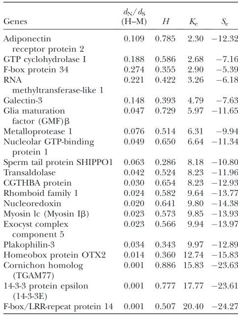
Table 1 shows the results. The dN/dS ratio varies substantially among genes (from 0.001 to 0.274), and theH-index ranges from 0.286 to 0.886. Consequently, the estimated effective number of molecular pheno-typesKeranges from 2.3 to 20.4, with an average of 8.77 (the median is 8.23). Our analysis suggests that most genes are highly pleiotropic. That is, there are on av-erage eight distinct components in the fitness that may be related to a gene. Roughly,73% of the among-gene variation in thedN/dSratio can be explained by the var-iation inKeamong genes. In other words, the level of gene pleiotropy associated with a gene may be the dom-inant factor for predicting sequence conservation, as predicted by Fisher(1930). The effective mean
selec-tion intensity (Se) ranges from 5.39 to 23.63, with a median of 12.6. Note thatdN/dSratios in Table 1 were estimated from the human and mouse orthologous genes; using other mammals or taking an average would lead to5% difference in theKeestimation.
DISCUSSION
Estimation of gene pleiotropy:Although the theory of gene pleiotropy, the capacity of a gene to affect multiple phenotypic characters, has been used to explain many
biological phenomena (Fisher 1930; Wright 1968;
Barton 1990; Waxman and Peck 1998; Otto 2004;
MacLeanet al.2004; Dudleyet al. 2005), the
character-istic level of pleiotropy remains largely unknown. Many phenotype–genotype models (e.g., Fisher1930; Wright
1968; Hartland Taubes1996, 1998; Waxmanand Peck
1998; Poonand Otto2000) have linked gene pleiotropy
to the dimensionality of the fitness function of the organism. The major contribution of this article is to for-mulate a statistical framework for estimating the capacity of a gene to significantly affect distinct components in the fitness, the effective number of molecular phenotypes (Ke). Thus, for the first time we have an empirical mea-sure of gene pleiotropy. Examples in Table 1 show thatKe is typically6–9, the number of distinct fitness compo-nents a gene may affect, which has been further con-firmed by a large-scale data analysis (not shown).
Our SM model provides an approach to understand-ing the role of gene pleiotropy in a gene network. Al-though a detailed analysis will be published elsewhere, we test the hypothesis that gene pleiotropy underlies genomic correlations related to the evolutionary rate of protein sequence (He and Zhang 2006; Palet al.
2006; Wolfet al. 2006). That is, (i) evolutionary rate is Figure 4.—Phylogenetic tree of vertebrates used in our
data analysis.
TABLE 1
Estimation ofKeandSefor 20 vertebrate proteins
Genes
dN/dS
(H–M) H Ke Se
Adiponectin
receptor protein 2
0.109 0.785 2.30 12.32
GTP cyclohydrolase I 0.188 0.586 2.68 7.16 F-box protein 34 0.274 0.355 2.90 5.39 RNA
methyltransferase-like 1
0.221 0.422 3.26 6.18
Galectin-3 0.148 0.393 4.79 7.63 Glia maturation
factor (GMF)b
0.047 0.729 5.97 11.65
Metalloprotease 1 0.076 0.514 6.31 9.94 Nucleolar GTP-binding
protein 1
0.049 0.650 6.64 11.34
Sperm tail protein SHIPPO1 0.063 0.286 8.18 10.80 Transaldolase 0.042 0.524 8.23 11.96 CGTHBA protein 0.030 0.654 8.23 12.93 Rhomboid family 1 0.024 0.582 9.64 13.77 Nucleoredoxin 0.020 0.641 9.80 14.38 Myosin lc (Myosin Ib) 0.023 0.573 9.85 13.93 Exocyst complex
component 5
0.023 0.566 9.94 13.97
Plakophilin-3 0.034 0.343 9.97 12.89 Homeobox protein OTX2 0.014 0.360 12.74 15.83 Cornichon homolog
(TGAM77)
0.001 0.886 15.83 23.63
14-3-3 protein epsilon (14-3-3E)
0.001 0.777 17.77 23.61
F-box/LRR-repeat protein 14 0.001 0.507 20.40 24.27
ThedN/dSratio was calculated from the human (H) and
inversely related to gene pleiotropy (K), (ii) gene pleiotropy determines gene dispensability, and (iii) gene pleiotropy underlies ‘‘hub’’ genes. In short, estimation of gene pleiotropy (Ke) provides a model-based data-analysis approach that avoids the interpretative difficulty in principle-component or partial-correlation analysis.
In the future, we shall refine the analytical pipeline for estimatingKe. We shall examine how statistical proper-ties ofdN/dSandHwould affect the estimation efficiency ofKe. In addition to the delta method, another method to estimate the sampling variance of the estimatedKeis nonparametric bootstrapping. Under theW-model when the selection intensitySfollows a (negative) gamma dis-tribution, a likelihood approach can be developed. Since the method of Nielsen and Yang (2003) is applicable
only for closely related sequences, we shall develop a protein sequence-based likelihood approach.
Gene pleiotropy and allelic pleiotropy: It should be noted that the effective number of molecular pheno-types (Ke) measures the functional pleiotropy of a gene, rather than a single mutation. For instance,Ke¼8.23 for trans-aldolase is the estimated number of distinct fitness dimensions implied by all random mutations in the coding sequence. Although the estimatedKeindicates that most genes may be highly pleiotropic, what it exactly means is very much gene specific.
The number of fitness dimensions affected by a single mutation (V) could be much less than Ke, say, 2–4 (Dudleyet al. 2005). Waxmanand Peck(1998) argued
that a single optimal gene sequence may become common when three or more characters (as molecular phenotypes here) are affected by each mutation, (i.e.,V $3). The problem of estimatingVeffectively from sequence data remains a question that requires further study.
Several studies (Nielsenand Yang 2003; Piganeau
and Eyre-Walker 2003; Eyre-Walker et al. 2006)
estimated the shape parameter of gamma distribution for S. Nielsen and Yang (2003) obtained the shape
parameter of 3.22 from the primate mitochondrial ge-nome sequences. Under the SM framework, it can be interpreted as Ke/2; see the above section for the
W-model. That is,Ke¼233.22¼6.44 for primate mi-tochondria proteins, consistent with our results (Table 1). In contrast, Eyre-Walkeret al. (2006) obtained a much
smaller value (0.23) of the shape parameter from the human SNP data. We speculate that the estimate from population genetics data perhaps reflects the allelic pleio-tropy (V). Hence, Eyre-Walkeret al.(2006) may provide
a rough estimate forV¼230.23¼0.46.
Assumptions and alternative models: The SM model involves several simplifying assumptions, since an ex-haustive consideration of all possible mutational effects on molecular phenotypes is intractable. Many are shown with previous phenotype–genotype models. One may refer to Martin and Lenormand (2006) for a recent
summary about rationales and criticisms. The first as-sumption is the single fitness optimum. Under this
condition we assume that disruptive selection with alter-native optima following an adaptive process (reviewed in Kingsolver et al. 2001 and Elena and Lenski 2003)
occurs rarely at the molecular level. Moreover, we used the Gaussian fitness function (see Equation 1) to measure the fitness consequences of a deviation from the optimum. Lande(1980) showed that when the population mean is
close to the optimum, a Gaussian-like function can be a local kernel approximation for many arbitrary fitness functions.
Second, the effect of mutations on molecular pheno-types is assumed to be continuous and symmetric. The continuous property is consistent with some empirical evidence from random mutations of genes (Keightley
1994; Keightley and Caballero 1997; Imhof and
Schlotterer 2001). The symmetric assumption
im-plies that even if mutations bias toward higher or lower values of molecular phenotypes, the trend should be small compared to the mutational variance. In practice we used a multiple Gaussian distribution for mutational effects. In the non-Gaussian case, it is possible to reduce kurtosis after an appropriate transformation such that mutational effects on a ‘‘transformed’’ molecular phe-notype are roughly Gaussian-like. In short, we conclude that in the absence of practically useful alternatives, sin-gle optimum, Gaussian fitness function, and continuous symmetric effect of mutations remain useful working assumptions. Further work will examine the effects of these assumptions using computer simulations.
A more important issue is whether the estimation procedure for the effective number of molecular phe-notypes (Ke) is robust under various alternative models. The first alternative model is Fisher’s geometric model, in which adaptive change is represented by stepwise move-ment of a point toward the center of the hypersphere. In this case, the number of molecular phenotypes (K) is Fisher’s geometric dimension. Several studies (Hartl
and Taubes1996, 1998; Sellaand Hirsh2005) showed
that at equilibrium, Fisher’s geometric model can be approximated by allowing the current population to vary randomly around the fixed optimum. A second alterna-tive model is to define the fitness to be a function of flux through a metabolic pathway (Kacserand Burns1979;
Hartl and Taubes 1996), rather than a Gaussian-like
function. Preliminary results have indicated that in both cases, estimation ofKevaries only slightly. It seems thatKe is a robust measure of gene pleiotropy, which may not be very sensitive to the specific evolutionary model. We shall address this issue more extensively in future studies.
The author is grateful to Adam Eyre-Walker and the reviewing editor Antony Long for constructive comments on the manuscript. Assis-tance in data analysis from Dongping Xu and Zhixi Su is appreciated.
LITERATURE CITED
Bataillon, T., 2000 Estimation of spontaneous genome-wide muta-tion rate parameters: Whither beneficial mutamuta-tions? Heredity84: 497–501.
Drummond, D. A., J. D. Bloom, C. Adami, C. O. Wilkeand F. H. Arnold, 2005 Why highly expressed proteins evolve slowly. Proc. Natl. Acad. Sci. USA102:14338–14343.
Dudley, A., D. Janse, A. Tanay, R. Shamirand G. Church, 2005 A global view of pleiotropy and phenotypically derived gene func-tion in yeast. Mol. Syst. Biol.1:2005.0001.
Elena, S. F., and R. E. Lenski, 2003 Evolution experiments with mi-croorganisms: the dynamics and genetic bases of adaptation. Nat. Rev. Genet.4:457–469.
Eyre-Walker, A., M. Woolfitand T. Phelps, 2006 The distribution of fitness effects of new deleterious amino acid mutations in hu-mans. Genetics173:891–900.
Fisher, R. A., 1930 The genetical theory of natural selection. Oxford University Press, Oxford.
Gillespie, J. H., 1991 The Causes of Molecular Evolution.Oxford Uni-versity Press, Oxford.
Gu, X., and J. Zhang, 1997 A simple method for estimating the pa-rameter of substitution rate variation among sites. Mol. Biol. Evol. 14:1106–1113.
Gu, X., 2007 Stabilizing selection of protein function and distribu-tion of selecdistribu-tion coefficient among sites. Genetica (in press). Gu, X., Y. X. Fuand W. H. Li, 1995 Maximum likelihood estimation
of the heterogeneity of substitution rate among nucleotide sites. Mol. Biol. Evol.12:546–557.
Hartl,D.L.,andC.H.Taubes,1996 Compensatorynearlyneutralmuta-tions: selection without adaptation. J. Theor. Biol.182:303–309. Hartl, D. L., and C. H. Taubes, 1998 Towards a theory of
evolution-ary adaptation. Genetica102/103:525–533.
He, X., and J. Zhang, 2006 Toward a molecular understanding of pleiotropy. Genetics173:1885–1891.
Imhof, M, and C. Schlotterer, 2001 Fitness effects of advanta-geous mutations in evolving Escherichia coli populations. Proc. Natl. Acad. Sci. USA98:1113–1117.
Kacser, H., and J. A. Burns, 1979 Molecular democracy: Who shares the controls? Biochem. Soc. Trans.7:1149–1161. Kasprzyk, A., D. Keefe, D. Smedley, D. London, W. Spooneret al.,
2004 EnsMart: a generic system for fast and flexible access to biological data. Genome Res.14:160–169.
Keightley, P. D., 1994 The distribution of mutation effects of via-bility inDrosophila melanogaster.Genetics138:1315–1322. Keightley, P. D., and A. Caballero, 1997 Genomic mutation rates
for lifetime reproductive output and lifespan inCaenorhabditis elegans. Proc. Natl. Acad. Sci. USA94:3823–3827.
Kimura, M., 1979 Model of effectively neutral mutations in which se-lective constraint is incorporated. Proc. Natl. Acad. Sci. USA75: 1934–1937.
Kimura, M., 1983 The Neutral Theory of Molecular Evolution. Cam-bridge University Press, CamCam-bridge, UK.
Kingsolver, J. G., H. E. Hoekstra, J. M. Hoekstra, D. Berrigan, S. N. Vignieriet al., 2001 The strength of phenotypic selection in natural populations. Am. Nat.157:245–261.
Lande, R., 1980 The genetic covariance between characters main-tained by pleiotropic mutations. Genetics94:203–215. Lynch, M., J. Blanchard, D. Houle, T. Kibota, S. Schultzet al.,
1999 Perspective: spontaneous deleterious mutation. Evolution 53:645–663.
MacLean, R. C., G. Belland P. B. Rainey, 2004 The evolution of a pleiotropic fitness tradeoff in Pseudomonas fluorescens. Proc. Natl. Acad. Sci. USA101:8072–8077.
Martin, G., and T. Lenormand, 2006 A general multivariate exten-sion of Fisher’s geometrical model and the distribution of muta-tion fitness effects across species. Evolumuta-tion60:893–907. Nielsen, R., and Z. Yang, 2003 Estimating the distribution of
selec-tion coefficients from phylogenetic data with applicaselec-tions to mi-tochondrial and viral DNA. Mol. Biol. Evol.20:1231–1239. Ohta, T., 1973 Slightly deleterious mutant substitutions in
evolu-tion. Nature246:96–98.
Ohta, T., 1977 Extension to the neutral mutation random drift hy-pothesis, pp. 148–176 inMolecular Evolution and Polymorphism, edited by M. Kimura. National Institute of Genetics, Mishima, Japan. Otto, S. P., 2004 Two steps forward, one step back: the pleiotropic
effects of favoured alleles. Proc. Biol. Sci.271:705–714.
Pal, C., B. Pappand M. J. Lercher, 2006 An integrated view of pro-tein evolution. Nat. Rev. Genet.7:337–348.
Piganeau, G., and A. Eyre-Walker, 2003 Estimating the distribution of fitness effects from DNA sequence data: implications for the mo-lecular clock. Proc. Natl. Acad. Sci. USA100:10335–10340. Poon, A., and S. P. Otto, 2000 Compensating for our load of
mu-tants: freezing the meltdown of small populations. Evolution54: 1467–1479.
Shaw, F. H., C. J. Geyerand R. G. Shaw, 2002 A comprehensive model of mutations affecting fitness and inferences for Arabi-dopsis thaliana. Evolution56:453–463.
Sella, G., and A. E. Hirsh, 2005 The application of statistical physics to evolutionary biology. Proc. Natl. Acad. Sci. USA102:9541–9546. Turelli, M., 1985 Effects of pleiotropy on predictions concerning mu-tation-selection balance for polygenic traits. Genetics111:165–195. Uzzel, T., and K. W. Corbin, 1971 Fitting discrete probability
distri-bution to evolutionary events. Science172:1089–1096. Wagner, A, 2000 The role of population size, pleiotropy and fitness
effects of mutations in the evolution of overlapping gene func-tions. Genetics154:1389–1401.
Wagner, G. P., 1989 Multivariate mutation-selection balance with constrained pleiotropic effects. Genetics122:223–234. Wall, D. P., A. E. Hirsh, H. B. Fraser, J. Kumm, G. Giaeveret al.,
2005 Functional genomic analysis of the rates of protein evolu-tion. Proc. Natl. Acad. Sci. USA102:5483–5488.
Waxman, D., and J. R. Peck, 1998 Pleiotropy and the preservation of perfection. Science279:1210–1213.
Welch, J. J., and D. Waxman, 2003 Modularity and the cost of com-plexity. Evolution57:1723–1734.
Wolf, Y. I., L. Carmeland E. V. Koonon, 2006 Unifying measures of gene function and evolution. Proc. Biol. Sci.273:1507–1515. Wright, S., 1968 Evolution and the Genetics of Populations.University
of Chicago Press, Chicago.
Yang, Z., 1997 PAML: a program package for phylogenetic analysis by maximum likelihood. Comput. Appl. Biosci.13:555–556. Zhang, X. S., and W. G. Hill, 2003 Multivariate stabilizing selection
and pleiotropy in the maintenance of quantitative genetic varia-tion. Evolution57:1761–1775.
Communicating editor: A. D. Long
APPENDIX
Mean and variances ofS—derivation of Equations 13 and 14:For the distribution ofythat follows a multi(K )-variate normal distribution,
pðyÞ ¼ 1
ðpffiffiffiffiffiffi2pÞKjS
mj1=2
exp y9S
1 my
2
; ðA1Þ
we note that for any quadratic functiony9U1y, the first and second moments can be expressed as
E½y9U1y ¼tr U1Sm
E½ðy9U1yÞ2 ¼2 trðU1SmÞ21tr½U1Sm2
; ðA2Þ
respectively, where the operator tr[.] means the trace of a square matrix. From Equation 7 it is straightforward that
S ¼ 2Netr½U1Smand VarðSÞ ¼8Ne2tr ðU 1S
mÞ 2
. De-note the matrixA¼U1S
m. After noting that the trace of the matrix is the sum of the eigenvalues, i.e., tr½A ¼ PK
i¼1ai and tr½A2 ¼
PK
i¼1a2i, we obtain Equations 13
and 14.
Canonical representation of S—derivation of Equa-tion 15: The canonical representation will choose molecular phenotypes such that Sw ¼ diag(s2w,1, . . .,
s2
w;K). Recall thatA¼U
1Sm¼ZV, whereZ¼S1
andV¼S1w SmZ. Then, one can verify tr½Z ¼tr diag½
s2
w;1;. . .;s 2
w;K
Sm ¼PK
i¼1s2m;i=s2w;i, since the trace
of a matrix is the sum of its diagonal elements. Next,
matrix V can be written as V¼ diag s2
w;1;. . .;
s2
w;KÞ
2
SmSm. It follows that tr½V ¼
PK i¼1d
2
i=s
4
w;i,
where d2
i is the ith eigenvalue of matrix SmSm. From
the relation tr[A]¼tr[Z]tr[V], together we have
tr½A ¼X
K
i¼1 s2m;i s2
w;i
1 d
2
i
s2
w;is2m;i
!
¼X
K
i¼1 s2m;i s2
w;i
ð1giÞ;
ðA3Þ
leading to Equation 15, wheregi¼d2
i/[s
2
w;is
2 m;i].
The canonical form for the variance of S can be obtained similarly, but the algebra is somewhat tedious, largely due to the detail ofA2¼Z21 V22ZV. Let
M4
i ¼s4m;i1
PK j6¼is
2
m;ij. One thus can show the trace
tr½Z2 ¼PK
i¼1 Mi2=s2w;i
2
and tr½V2 ¼PK i¼1 d
2
i=s4w;i
2
.
Noting that ZV ¼ diag(s2
w,1, . . ., s2w,K)SmSmSm, we obtain tr½ZV ¼PK
i¼1b 3
i=s6w;i, whereb
3
i is theith
eigen-value of matrix SmSmSm. Therefore, from the fact tr[A2]¼tr[Z2]1tr[V2]2 tr[ZV], we have
VarðSÞ ¼8Ne2X
K
i¼1 Mi2 s2w;i
!2
1 d
2
i
s4w;i !2
2b
3
i
s6w;i
" #
: ðA4Þ
Condition of S-gamma distribution:Givenp(y) char-acterized by the covariance Sw, the distribution of
selection intensity,f(S), can be uniquely determined by the probability theory that for anyS* andy* that satisfy S* ¼ 2Ne(y*9S
1
w y*) in Equation 7, the relationship
ÐS*
fðSÞdS¼ 2Ne
Ðy*
y9S1w ypðyÞdyholds. However, the analytical form off(S) is not available, except for the case
when the matrix U in the quadratic form and the
covariance in p(y), Sm, satisfies A ¼ SmU1 ¼ aI. In other words, the matrixAis diagonal, having the same eigenvaluesa.
Moments of evolutionary rate—derivation of Equa-tions 20 and 21:Here we show several analytical integral results. First we considerI1¼
Ð
e2Ney9U1ypðyÞdy, which is given by
I1¼ ð‘
‘ . . .
ð‘
‘
e2Ney9U1y3exp y9S 1 my=2
ðpffiffiffiffiffiffi2pÞKjSmj1=2 dy
¼ jBj 1=2 jSmj1=2
ð‘
‘ . . .
ð‘
‘
exp½y9B1y=2 ðpffiffiffiffiffiffi2pÞKjBj1=2 dy¼
jBj1=2 jSmj1=2;
ðA5Þ
whereB¼ S1m 14NeU1
1
. It follows that
I1 ¼
jSm114NeU1j1=2
jSmj1=2 ¼ jI14NeU
1Smj1=2
¼ jI14NeAj1=2: ðA6Þ
In the same manner, we have I2 ¼
Ð
e4Ney9U1ypðyÞdy given by
I2¼ jI18NeSw1Smj
1=2¼ jI18NeAj1=2: ðA7Þ
Next we considerI3¼
Ð
½2Ney9U1ye2Ney9U
1y
pðyÞdy. From the derivation ofI1, one can verify
I3¼ jBj1=2 jSmj1=2
ð‘
‘ ...
ð‘
‘
ð2Ney9U1yÞexp½y9B
1y=2 ðpffiffiffiffiffiffi2pÞKjBj1=2 dy:
ðA8Þ
From Equation A2, we obtain
I3¼ jBj1=2
jSmj1=232Netr S
1
w B
¼2Netr S
1
mU14NeI
1
h i
jI14NeU1Smj1=2
¼2Netr½ðA
114NeIÞ1 jI14NeAj1=2
: ðA9Þ
In the same manner, we show that I4¼
Ð
½2Ney9U 1
y e4Ney9U1ypðyÞdyas follows:
I4¼
2Netr½ðA118NeIÞ1
jI18NeAj1=2 : ðA10Þ
Finally, we consider the integral I5 ¼
Ð
½2Ney9U1y2
e4Ney9U1ypðyÞdy. Similar to the derivations of I 1–I5, one can write
I5¼ jB*j1=2 jSmj1=2
ð‘
‘ ...
ð‘
‘
ð2Ney9U1yÞ2
exp½y9B*1y=2 ðpffiffiffiffiffiffi2pÞKjB*j1=2 dy
¼jB*j 1=2 jSmj1=2 8N
2 etr½ðU
1B*Þ21ð2
Netr½U1B*Þ2
;ðA11Þ
where matrixB*¼(S1m 18NeU1)1. SinceU1B* ¼ (S1m U18NeI)1¼(A118NeI)1, andjB*/Smj ¼ jI1 8NeAj,I5can be written as follows:
I5¼jI18NeAj1=2
3 8Ne2tr½ðA118
NeIÞ21ð2Netr½A118NeIÞ2
:
ðA12Þ
From Equation 19, one can show thatl=v¼I11cI3 and
l2=v2¼I