A Novel Solution Approach to Capacitated Lot-Sizing Problems with Setup Times and Setup Carry-Over.

(1)

ABSTRACT

KARAGUL, HAKAN FATIH. A Novel Solution Approach to Capacitated Lot-Sizing Problems with Setup Times and Setup Carry-Over. (Under the direction of Donald P. Warsing and Thom J. Hodgson.)

In this study we propose a novel mixed integer linear programming (MILP) formulation to solve capacitated lot-sizing problems (CLSP) with setup times and setup carry over. We compare our novel formulation to two formulations in the literature by solving single- and multiple-machine instances with and without holding costs. We refer to one of these original formulations as the ―classical formulation,‖ and we call the other, which is modified from the classical formulation, the ―modified formulation.‖ Extensive

(2)

(3)

(4)

A Novel Solution Approach to Capacitated Lot-Sizing Problems with Setup Times and Setup Carry-Over

by

Hakan Fatih Karagul

A dissertation submitted to the Graduate Faculty of North Carolina State University

in partial fulfillment of the requirements for the Degree of

Doctor of Philosophy

Industrial Engineering

Raleigh, North Carolina 2012

APPROVED BY:

_______________________________ ______________________________

Thom J. Hodgson Donald P. Warsing

Committee Co-Chair Committee Co-Chair

________________________________ ________________________________

(5)

ii DEDICATION

This thesis is dedicated to My Mother, Ayfer

My Father, Hasan My Brother, Huseyin Iskender

and

(6)

iii BIOGRAPHY

(7)

iv ACKNOWLEDGMENTS

This dissertation would not have been possible without the invaluable guidance and support of my advisors Dr. Donald Warsing, Dr. Thom J. Hodgson, Dr. Reha Uzsoy and Dr. Russell E. King. I am thankful that they believed in me and gave me the chance to work on this project.

I would like to thank Dr. Sudhendu Rai and Kenneth Mihalyov from Xerox Corporation for their generous support. I am grateful to them for the invaluable feedback they provided during this research.

I would also like to thank my friends Dr. Erinc Albey, Dr. Yasin Alan and Dr. Ali Kefeli for their collaboration, input and support. I thank my friends Nils Buch, Kuang-Hao Buch, Peter Prim, Sean Carr, Krishna Jarugumilli, Emine Yaylali, Dr. Jennifer Mason, Dr. Benjamin Lobo, Dr. Jeremy Tejada, Dr. Bjorn Berg and Dr. Baris Kacar for providing a great atmosphere in the Department of Industrial and Systems Engineering at NC State University.

(8)

v

CHAPTER 1

1 INTRODUCTION

Production planning problems can be categorized into three areas: High-level, medium-level and low-level planning problems. In high-level production planning activities, decisions are made regarding total production capacity and/or resource levels to support production, while medium-level activities mostly deal with production lot-sizing decisions. By solving lot-sizing problems, planners determine how much to produce and in which period to produce. Low-level production problems are known as scheduling or sequencing problems, where the complete sequence of the jobs is determined for different periods in a production horizon.

(17)

2 capacitated lot-sizing problems for an arbitrary number of periods and an arbitrary number of production orders (jobs) on both a single machine and across multiple, identical machines running in parallel. We first formulate our motivating problem, a transactional print-shop problem, as a special case of the CLSP and then extend our formulation to solve general CLSP.

The transactional print-shop problem that serves as the motivating problem for this research concerns a production environment in which customers place orders in ―groups‖ (or families) whose component jobs may have multiple deadlines. For example, a customer may order 100 units of product (i.e., 100 printed copies), but request that 50 units be delivered in three days, 30 units the day after that, and 20 units the day after that. This demand structure is typical of transactional printing services—e.g., in the printing of various periodic statements like cable television billing statements or health insurance ―EOBs‖ (―explanation of benefits‖ forms). This multiple-deadline ordering structure quite likely stems from the

fact that the producer (print shop) and its customers both recognize that the totality of each customer’s order, or perhaps the orders of just a few customers, would likely consume all of the producer’s capacity in the short term. Therefore, the customers are willing to alter their ordering behavior to reflect the fact that each order can be delivered in ―chunks‖ that spread

(18)

3 volume, and with some setup time possibly required at each operation to switch from one job group (customer order, job family, or product) to the next.

Since this problem can be interpreted as either a scheduling problem or as a lot-sizing problem, we provide an overview of both bodies of literature in the next section, followed by the problem overview.

1.1 Literature Review

In this section we look at two strands of literature by first reviewing the lot-sizing literature and then the scheduling literature.

1.1.1 Lot-Sizing Literature

In production systems, lot-sizing decisions are being made continually and have a direct impact on operating costs. If planning horizons are long and inventory holding costs are high, lot-sizing decisions may be critical to reducing inventory costs. Lot-sizing decisions can also be critical to minimizing non-value-added processes like setups. Being able to achieve this goal is important if the cost of resources (machines) and the cost of setups are high. Indeed, print shops are a good example of such an environment. Since industrial printers are relatively expensive machines, they should process jobs continuously in order to meet the return-on-investment goals of the company. Moreover, compared to the printing process, setting up the machine is a laborious process, and therefore it is desirable to minimize setups.

(19)

4 Ritzman and Bahl [13] presented classical capacitated lot-sizing formulations. Bitran and Yanasse [14] proved that CLSP is NP-Hard even if setup times are not taken into account. Maes [15] worked on the feasibility problem and demonstrated that this problem is NP-Complete.

It should be noted that none of these studies above considers ―setup carry-overs‖, also referred to as ―linked lot-sizes‖. A setup is carried over to the next period when the last job of

(20)

5 al. [22] and Meyr [23], who reviewed scheduling and lot-sizing decisions for big-bucket and small-bucket problems. A lot-sizing problem is called a small-bucket problem if its solution determines the complete sequence of the jobs; otherwise it is called a big-bucket problem. CLSP falls into the big-bucket category since it doesn’t determine the complete sequence of jobs.

1.1.2 Scheduling Literature

In the last two decades many researchers have investigated single-machine scheduling problems involving setup times. If some jobs from the same group (or family) can be combined into a single batch to eliminate setup times, then the literature calls the problem a batch setup problem; otherwise, the problem is called a non-batch setup problem [1]. Two main types of batch-setup problems are defined in the literature: ―batch-availability formulations‖ and ―job-availability formulations.‖

In batch-availability formulations it is assumed that a job in a batch becomes available when processing of all jobs in that particular batch is completed. In job-availability formulations the completion time of each job in a particular batch is independent from other jobs in the same batch [2]. In this study we focus on batch setup problems with job availability. Another important issue is setup time characteristics. Setup times might depend on the sequence of jobs or they can be independent of such a sequence. We assume that setup times are sequence-independent.

(21)

6 computational experiments that this measure of performance generates ―high quality‖

schedules under certain conditions [3]. Since most of these problems are NP-Hard [4], heuristic solutions are suggested in many cases. Baker [5] demonstrated that earliest-due-date sequencing yields the optimum solution if setup times are negligible, and a group technology approach (jobs from same family are grouped in a single batch) works well if setup times are relatively long and/or if the due dates are identical. Baker [5] also developed a gap heuristic and a neighborhood search approach for performance improvement. Uzsoy and Velásquez [6] improved existing heuristics for this problem and analyzed their performance. In this study, we focus on problems with no late job constraints, meaning that if a job is not completed before its deadline, then the schedule is infeasible. In this case minimizing maximum lateness leads to many optimal solutions which can potentially be improved further in terms of the total setup cost.

In the motivating context for this research (transactional print shops), inventory holding costs are not significant compared to setup costs. In addition, setup costs and setup times are the same for all jobs on each machine. Under these assumptions, objectives such as minimizing the total setup time, maximizing the setup savings, minimizing the make-span, minimizing the total number of setups or minimizing the maximum completion time yield similar results. In this group of objectives the main goal is to batch as many jobs as possible. In the second chapter of this dissertation, our main concern is minimizing the total setup cost. In the third chapter we extend our objective function by including holding costs.

(22)

7 technology approach will give the optimum solution. Unal and Kiran [8] developed an exact algorithm to find a feasible schedule for the feasibility problem formulated by Bruno et al. [7]. Driscoll et al. [9] suggested a dynamic programming approach to minimize the total changeover cost. However, that study assumes that setup times are negligible. It should be noted that dynamic programming approaches proposed in these papers can be used to solve small problems, but they are not practical for relatively large problems. For instance Monma and Potts [10] showed that the computational complexity of their dynamic programming algorithm is exponential in the number of job families.

In this study we present a novel mixed-integer-programming (MIP) formulation to solve capacitated lot-sizing problems with setup carry-overs. This novel formulation is a fixed charge network flow interpretation of the problem. We show that our novel formulation outperforms the formulations in the literature.

1.2 Problem Overview

(23)

8 There are T periods in the horizon. In our case these periods are considered to be weekdays. This is reasonable because in many industries, including the printing industry (the original motivation for this work), deadlines are defined by days and not by, say, hours. Each order can have up to T jobs with different deadlines. A job can be due only at the end of a period. In other words if we have T periods, we have only T different deadlines defined in our problem. If the deadline of a job is period t, then the job must be completed by the end of period t. Based on our experience, this ordering structure is not uncommon, especially in print shops. We refer to each order as a ―family,‖ and no setup is required between jobs from

the same family. If the next job is not from the same family as the current job, then a setup is required. As mentioned above we also consider setup carry-overs between periods. We assume that a setup cannot start in one period and complete in the next period. Before generating the schedule, orders are clustered first. If there are two jobs from the same family due in the same period, we batch them and consider them as a single job because having two setups in a single period for jobs from the same family does not serve our objective. Another assumption we make in this study is that there is no machine breakdown. This means at all points in time the machine (or the machines) is available for set-up or processing jobs.

(24)

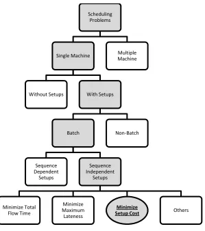
9 Figure 1 - Scheduling Literature Map

We know that if the number of product families is large, the chance of producing only a single type of product in an entire period decreases in the optimal solution. If one knows that production of a single type of product in an entire period is unlikely, then he/she can restrict the setup carry-overs in the formulation. By restricting the carry-overs we mean that a setup can be carried over to the next adjacent period but no further. In [17], Haase names the formulation with such a restriction ―Capacitated Sizing Formulation with Linked Lot-Sizes of Adjacent Periods‖.

Scheduling Problems

Single Machine

Without Setups With Setups

Batch

Sequence Dependent

Setups

Sequence Independent

Setups

Minimize Total Flow Time

Minimize Maximum Lateness

Minimize

Setup Cost Others

(25)

10 Haase shows that this restriction improves the performance of the formulation significantly. Transactional print-shops receive hundreds of orders daily and based on our experience, in transactional print-shops more than one type of job gets processed in each period (defined as ―day‖ or ―shift‖), so this assumption is reasonable. In other words, in the

single-machine formulation we assume that the processing time of a single job is always less than the period capacity. Throughout this study, when we say ―performance‖ we mean the computation time and the gap between the upper and lower bounds from the branch-and-bound tree, as reported by CPLEX (v. 12.2).

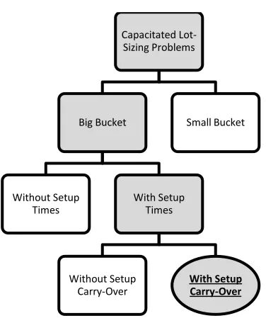
Figure 2 presents where our problem formulation (shown in bold) fits in the lot-sizing literature.

Figure 2 - Lot-Sizing Literature Map Capacitated

Lot-Sizing Problems

Big Bucket

Without Setup Times

With Setup Times

Without Setup Carry-Over

With Setup Carry-Over

(26)

11

1.3 Problem Notation and Properties

In order to define some important properties of the problem we consider in this research, we first formally define the parameters that are relevant to the problems studied.

P: Number of job families (products), P{1,..., }P

T: Number of periods, T {1,..., }T

1 if job is due in period 0 otherwise

tp

p t

y  



u p

t : Process time per unit of product p

s p

t : Setup time of product p

pt

d : Demand volume of product p in period t

t

C : Capacity (i.e. total time available) in period t

An important property of these problems is what we define as the density,



, given by

tp t T p P

y

TP

 _



 

,

[0

 



1]

(1)

Density is a measure of the extent to which the ―jobs matrix‖ is filled. If every job

(27)

12 which is the maximum number of jobs possible. In that case  1. If there are no jobs at all

then



_{is equal to 0. In other words, based on its definition,}0 



1.

Another important property of these problems is the slackness,_t, given by





1

u s

p pt p pt p P

t

t d t y

C

 



 



(2)

Since our procedures attempt to save setup time by moving jobs from later periods into earlier periods, the slackness defined in (2) is a measure of the minimum proportion of time available in period t into which jobs could be moved. We note, however, that this measure of slackness underestimates time available since it assumes the maximum number of

setups required to complete the schedule. It should be also noted that _t can have negative

values. We use slackness and density parameters later in generating problem instances for our computational tests.

(28)

13 last jobs in a period is determined. All three formulations minimize the total setup cost subject to no tardy jobs. At the end of Chapter 2, results are analyzed for a large set of computational experiments. Extensive computational tests show that our novel formulation and modified formulation outperform the classical formulation. We show in this chapter that the branch and bound tree of the modified formulation has fewer nodes compared to the classical formulation. We also demonstrate mathematically that the reason that the LP relaxation of our novel formulation provides better lower bounds compared to the classical and modified formulations is that the novel formulation results in tighter inequalities on some key constraints in the problem.

In Chapter 3, we extend our novel formulation so that it contains inventory variables and inventory holding costs. We test all three formulations (classical, modified and novel) using the test bed generated by Trigeiro et al. [11]. Results show that our novel formulation outperforms the modified formulation and the classical formulation.

(29)

14

CHAPTER 2

2 SINGLE-MACHINE FORMULATIONS

WITHOUT HOLDING COST

(30)

15 showing the equivalency of these three formulations can be found in Appendix A. Our approach is similar to the variable redefinition method proposed by Eppen and Martin in [24].

Before going into the details of the MILP formulations we define the parameters and the decision variables using the notation of Quadt and Kuhn [20]. Their review also includes some extensions that we point out here.

Parameters

i p

c Inventory holding cost of product p, in dollars per unit per period

s p

c Setup cost of product p, in dollars per setup.

0

p

I On-hand inventory of product p at the beginning of the planning horizon

R Big number, max{ }_t

t T

R C





Decision Variables

pt

x Amount of product p produced in period t

pt

I On-hand inventory of product p at the end of period t

1 if a setup is performed for product in period ; 0 otherwise

pt

p t

 _{ }



1 if the setup of product is carried over from period to period 1; 0 otherwise

pt

p t t

 _{ } 

(31)

16

2.1 Classical Restricted Capacitated Lot-Sizing Problem (CRCLSP)

The classical lot-sizing problem with restricted carry-overs is formulated as follows:

CRCLSP:

Minimize ₍ i s ₎

p pt p pt p P

t T

c I c 

  



₍₃₎ Subject to , 1

p t pt pt pt

I _ x d I  _p _{P t}_, _T (4)

( up pt sp pt) t p P

t x t  C



 



_{ }

_{t T}

(5)

, 1

( )

pt pt p t

x R   _  _p _{P t}_, _T ₍₆₎

0 0

0 , 0

p p p p

I I    _p _P (7)

0 , 0

pt pt

x  I   _p _{P t}_, _T ₍₈₎

1 pt p P   



_{ }

_{t T}

(9)

0

pt pt

   _{ }_p _{P t}_, __T ₍₁₀₎

, 1 1

pt p t

     p P t, T (11)

{0,1} , {0,1}

pt pt

(32)

17 This CRCLSP formulation minimizes the total holding and setup cost. As we mentioned earlier, we assume that holding cost is not significant in the motivating context

(transactional print shops), and therefore in this case, cip 0, p. Constraint (4) is the

inventory balance equation. Constraint (5) limits the sum of total setup time and total processing time in period t according to capacity available in the corresponding period. Constraint (6) assures that the machine is either set up or the setup is carried over from the previous period if there is production of product p in period t. Constraint (7) establishes the initial inventory and setup state. In our case we assume that the initial inventory is zero since

we consider a make-to-order system. We assume that 0

0,

p p

   meaning that no setup has

been carried over from previous periods to the first period of the problem. In other words, the machine is not set up for any product at the beginning of the planning horizon. Constraint (9) ensures that no more than one setup is carried over from one period to the next. Constraint (10) implies that the machine has to be set up in a period to be able to carry that setup to the next period. Constraint (11) implies that the setup can be carried over to the next adjacent period but not further.

2.2 Modified Restricted CLSP (Capacitated Lot-Sizing Problem)

(33)

18 our problem. Although the number of variables remains the same, the average computation time of this modified formulation is significantly less than that of the classical formulation.

In this formulation we redefine the setup variable _ptand change the notation

slightly. We replace the variable _ptin the classical formulation with the variable'_pt. While

pt

 represents the setup state _pt represents the production state. In other words, if a product

p_{is produced in period}t then _pt 1, else _pt 0.

Figure 3 and Figure 4 below show the difference between the two variables _pt and

pt

 . In both situations, a setup for product p=1 is carried over from the first period to the

second. Because the setup is carried over, the variable ₁₂ in the classical formulation is

equal to zero since there is not a set-up for product 1 in period 2. However the variable ₁₂ in

(34)

19 S p=1

S p=2 p=2 p=1

Period 1 Period 2

C1 C1 + C2

0

Slack

11 1

  12 1 11 1

 

Figure 4 - Modified Formulation S p=1

S p=2 p=2 p=1

Period 1 Period 2

C1 C1 + C2

0

Slack

11 1

  12 0 11 1

 

(35)

20 According to the new variable definition we make the following modifications:

 Replace constraint (5) in CRCLSP with

, 1

( up pt sp 'pt ps p t ) t p P

t x t  t   C



  



_{ }

_{t T}

(13)

 Replace constraint (6) with

'

pt pt

x R  _p _{P t}_, _T (14)

 Remove constraints (10) and (11). Add the following setup carry-over constraint to

the formulation:

, 1 , 1

2_pt _{p t}_ '_pt'_{p t}_ 0  _p _{P t}_, _T ₍₁₅₎

This constraint implies that the setup for a product p in period t can only be carried over to period t1 (_pt 1,'_{p t}_,_₁ 1), if product p is produced in period t ('_pt 1)

and if the setup for product p has not been carried over to period t from the previous period t1 (_{p t}_,_₁0).

 Replace constraint (12) with:

{0,1} , {0,1}

pt pt

    _{ }_p _{P t}_, __T (16)

 Replace the objective function with:

Minimize ( i_p _pt s_p '_pt s_p _pt)

p P t T

c I c  c 

 

 

(36)

21 We modify the objective function to take into account the setup cost saving due to setup carry-over. The complete formulation is as follows:

Modified Restricted CLSP (MRCLSP)

Minimize

1 ( i_p _pt s_p '_pt s_p _pt )

p P t T

c I c  c  _

   



(17) Subject to , 1

p t pt pt pt

I _ x d I  _p _{P t}_, _T (4)



' , 1



u s s

p pt p pt p p t t

p P

t x t  t   C 

  



_{ }

_{t T}

(13)

'

pt pt

x R  _p _{P t}_, _T (14)

0 0

0 , 0

p p p p

I I    p P (7)

0 , 0

pt pt

x  I   _p _{P t}_, _T (8)

1 pt p P   



_{ }

_{t T}

(9)

, 1 , 1

2_pt _{p t}_ '_pt'_{p t}_ 0  _p _{P t}_, _T (15)

'_pt {0,1} , _pt {0,1}

(37)

22

2.3 Novel Formulation

The novel formulation solves the same problem as the classical and modified formulations. It can be interpreted as follows: Assume that all jobs are initially allocated in their respective demand-periods (―lot-for-lot‖ plan) on a virtual uncapacitated machine. The novel mixed-integer program effectively takes the jobs from the virtual machine and allocates them to appropriate periods on the real machine so that the total setup cost is minimized. It should be noted that feeding the data into the MIP as it is given in the problem definition implies starting with the ―lot-for-lot‖ plan. So, there is not an additional step, but simply a formal statement of the initial demand data for the problem. Moving the jobs from a virtual machine to a real machine simply allows a visual interpretation of the model as an aid to understanding the problem formulation and solution.

The novel formulation starts with a ―lot-for-lot‖ plan and tries to improve it by making ―left-shifts‖. By ―lot-for-lot,‖ we mean processing each job in its demand period without batching it with jobs from the same family in other periods. ―Left-shift‖ is a common

(38)

23 possible period. The lot-for-lot plan might not be feasible due to capacity limitations, but if there is a feasible plan then the novel formulation makes necessary left-shifts and finds it.

Note that the problem data is preprocessed before solving this mixed integer program by batching the jobs with the same deadline and same product family. The solution to the MIP then determines what portion of which jobs must be moved from latter periods to earlier periods, and which jobs must be placed on the period boundaries to exploit setup carry-overs. Additional Parameters for Novel Formulation

1 if product is due in period ; 0 otherwise

tp

p t

y   

R: Big number R is equal to the total number of periods T

Additional Decision Variable for Novel Formulation

tkp

z : The portion of job p that is moved from its demand period k on the virtual machine to

period t on the real machine, 0 z_tkp 1 . The new variable z_tkp is only defined for kt.

That means that, to prevent deadline violations, we do not allow the jobs to be moved from their original demand period to later periods.

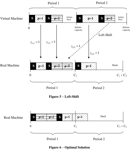
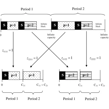
Figure 5 shows how the jobs on the virtual, uncapacitated machine are allocated to the real machine. The dashed line represents the ―left-shift‖. What we mean by z₁₂₂1 is that

the entire job of product two due in period 2 is ―left-shifted‖ to period 1. Since a lot-for-lot plan assumes that the job is processed in its demand period, no ―right-shifts‖ are allowed

(39)

24

kt. The other three vertical lines demonstrate that those jobs are not left-shifted and will be produced in their demand-periods.

Figure 6 – Optimal Solution Figure 5 – Left-Shift

S

S p=1 S p=2 p=2 p=1

Period 1 Period 2

C1 C1 + C2

0

Slack

S

S p=1 S p=2 S p=1 p=2

Period 1 Period 2

Infinite capacity Infinite capacity 0 Infinite Slack Infinite Slack 111 1 z  111 1 z  112 1 z  111 1

z  z1221 111 1 z  221 1 z  111 1 z  Virtual Machine Real Machine Left-Shift

S p=1

S p=2 p=2 p=1

Period 1 Period 2

C1 C1 + C2

0

Slack

(40)

25 Figure 6 shows how the plan looks after the job for product 2, due in period 2 is left-shifted from period 2 to period 1. If the sequence of the jobs in period 1 is changed, the setup for product 1 in period 1 can be carried over to period 2. In that case the plan looks like Figure 6. This is optimal because we know that there has to be at least one setup for each product. Since we have two products to produce, the plan with two setups has to be optimal.

Novel Formulation for CLSP NMCLSP

Minimize

1 ( s_p '_pt s_p _pt )

p P t T

c  c  _

  



₍₁₈₎ Subject to , 1 '

u s s

p tkp pk p pt p p t t

p P k T

t z d t



t



_ C

 

 _ _ _

 

 

 

t T



(19)

' '

tkp pt

k T

z R 







 p P t, T (20)

1 pt p P   



_{t T}

_

(21)

, 1 , 1

2_pt _{p t}_ '_pt'_{p t}_ 0  _p _{P t}_, _T (22)

tkp kp

t T

z y







 p P k, T (23)

0 0

p p

(41)

26 0z_tkp1  _p _{P t}_, _{T k}_, _T ₍₂₅₎

{0,1} , ' {0,1}

pt pt

    _{ }_p _{P t}_, __T ₍₂₆₎

Constraint (19) assures that capacity conditions are met. Constraint (20) forces a setup for product p in period t if any job is moved into period t of the real machine from the virtual machine. Constraints (21) and (22) take care of setup carry-overs as described in the previous section on the modified formulation with setup carry-overs. Constraint (23) ensures that all the jobs on the virtual machine are moved to the real machine. In other words, this constraint makes sure that the demand is satisfied. Note that the formulation does not allow production of more than the total demand because we know that in an optimal solution this is never the case since we assume a make-to-order environment. Constraint (24) defines the initial setup state. We assume that _p₀0, meaning that no setup has been carried over to

the first period. Constraint (25) defines the boundaries of variable z_tkp. Constraint (26) is the

integrality constraint for the other variables. The objective function of the novel formulation is the same as the objective function of the modified formulation; both are minimizing the total setup cost. We do not track inventory levels in this version of the novel formulation. Hence, there are no inventory variables. In next chapter, we extend the novel formulation so that it includes inventory holding costs in the objective function and therefore inventory variables are needed to track the inventory levels.

(42)

27 interpretation of our novel formulation for a single product for a three-period problem. Nodes 1, 2 and 3 represent the first three periods of the problem. Arcs (0,t) represent demands due in period t. They ensure that the problem starts with the lot-for-lot plan. Arcs (t,4) represent the production in period t and the flow of these arcs are given by the variable x_pt. The

variable x_pt represents the sum of processing times and the setup times in period t. In a

feasible solution, the capacity constraint requires that pt t,

p P

x C t



  



. It can be said that node

4 is the coupling node since different networks of different products are connected to each other through this node. It should be noted that in this fixed charge network flow diagram we do not show the variables z_tkpwhere t=k since arcs (0,t) already represent them.

Figure 7 - Fixed Charge Network Flow Interpretation of Novel Formulation

0 1 2 3 4 1 p x 2 p x 3 p x d1 d2 d3

d2*z12

d3*z23 d3*z13

1

s p

t  (Cost: cs_p)

3

s p

t  (Cost:cs_p)

(cost: S)

1

s p

t  (Cost:-cs_p)

2

s p

t  (Cost:-cs_p)

2

s p

(43)

28

2.4 Computational Experiments

In this section, first we explain how sample instances are generated for test purposes and then report the results of these computational experiments, followed by performance evaluations of the different formulations.

Density  and slackness _t_{are two important characteristics of demand structure and} both parameters are defined formally in Section 1.3. Other than these two parameters, number of periods, number of job families, job-size distribution and setup times are also significant problem characteristics.

In the first computational experiment, we assume that the processing times of jobs are uniformly distributed between 100 and 200. In the second experiment, we sample the processing times from two different uniform distributions to mimic the ―skewed‖

(44)

29 Table 1 - Sample Problem Characteristics

Parameter Values of Different Levels

T Number of Periods 5

P Number of Job Families 60, 100, 140

 Density 0.5, 0.7, 0.9

t

 Slackness 0, 0.25, 0.5

s p

t Setup time 10, 50, 100, 200

t

C Period Length (capacity)





1

u s

p pt p pt p P

t

t d t y











u p pt

t d Job Size

U

[100, 200]

We have a 3×3×3×4 full factorial design, and we generate 10 instances for each combination. So, in total, 1080 instances are solved using the three different formulations. All formulations are generated in Matlab 2010a and CPLEX 12.2 is used as the solver. We limit the number of active threads in CPLEX to one. Other than that, the CPLEX default settings are used. All experiments were run on a PC with an Intel Xeon 2.67 GHz CPU and 3 GB RAM.

2.4.1 Experiment with the Uniform Processing Times

In the first experiment processing times are generated using a single uniform

distribution,

U

[100, 200]

. After we show how the sample instances are generated we present

(45)

30 2.4.1.1Sample Instance Generation (Uniform Distribution)

Before presenting the algorithm used to generate sample instances, we must define a new parameter:

[ ]_t

E  

For our experiments,



is calculated simply by taking the average of _t. In addition, s p

t is

fixed and s s, p

t t pmeaning that [ ]s s p

E t t . In other words, setup time is the same for all

products. Also u p pt

t d is uniformly distributed between 100 and 200 implying that

[ up pt] 150

E t d  . Microsoft Excel 2007 and its standard functions are used to generate sample

problems.

The following procedure is used to generate sample problems for given values of  and



:

STEP 1: Generate a T × P matrix with random numbers

U

[0,1]

in each cell.

STEP 2: If the random number in a cell is greater than  , then set the cell value equal to 0, otherwise generate a processing time u

p

t from

U

[100, 200]

.

STEP 3: Set



[ ] [ ]



,

1

u s

p pt p

t

P E t d E t

C  t

 

 

 .

(46)

31 Table 2 - Test Bed Statistics (Slackness)

0

   0.25  0.5

P Min Max Mean Min Max Mean Min Max Mean 60 -0.06 0.15 0.03 0.14 0.37 0.25 0.44 0.58 0.50 100 -0.04 0.12 0.02 0.19 0.34 0.25 0.42 0.55 0.50 140 -0.03 0.09 0.02 0.20 0.31 0.25 0.45 0.55 0.50

Table 3 - Test Bed Statistics (Density)

0.5

   0.7  0.9

P Min Max Mean Min Max Mean Min Max Mean 60 0.41 0.57 0.49 0.63 0.75 0.69 0.84 0.94 0.90 100 0.44 0.58 0.49 0.62 0.74 0.70 0.82 0.93 0.89 140 0.45 0.55 0.50 0.65 0.74 0.70 0.86 0.93 0.90

2.4.1.2Experimental Results

We have two measures of solution performance: computation time and the percentage gap between the upper and lower bounds of the branch & bound tree. We report the default gap value returned by the CPLEX engine. The gap  is defined as follows:

100%.

UB LB

UB

z z z





  

The term z_UB defines the objective value of the current best integer solution (incumbent

solution) while *

LB

z represents the objective value of the LP relaxation optimal solution

(47)

32 We stop the solution engine after 1200 seconds and return the best solution found up to that point. We assume that in most real production environments, where production plans are regenerated frequently (e.g., every day or every shift), a computation time greater than 1200 seconds is not very practical. The other reason is the limited memory of personal computers. As expected, as the maximum computation time goes up, the more likely it is that the solution procedure will abort due to insufficient memory.

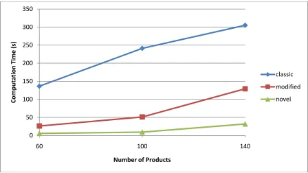
Table 4 shows the means, medians and standard errors of computation times (i.e., the standard deviation of the mean computation time, given by the sample standard deviation divided by the square root of the number of observations) for different formulations and different numbers of products. Please note that for each product level we solve 360 instances with a planning horizon of 5 periods. Clearly, the classic formulation performs worst among these three formulations.

Table 4 - Computation Time Summary, Single Machine, Uniform Processing Times

Time (s)

Classic Formulation Modified Formulation Novel Formulation

P Mean Std. Error Median Mean Std. Error Median Mean Std. Error Median

60 289 26 5 128 18 2 30 9 1

100 492 30 50 288 25 10 79 13 5

(48)

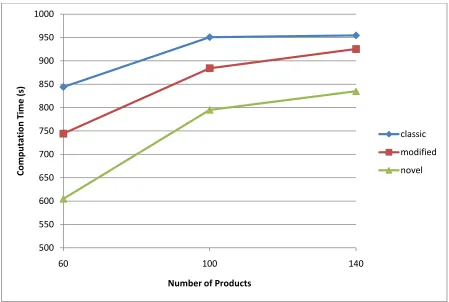
33 Figure 8 is the graphical representation of Table 4. The novel formulation seems to perform best. Although the difference is not pronounced for small problem instances, as the problem size increases, the performance difference becomes quite pronounced.

Figure 9 gives us a good sense of the computation time of instances that can be solved to optimality. However, it does not provide any information about the instances that cannot be solved to optimality. We also need to analyze comparative values of . In other words, we need to analyze the gaps remaining between the upper bound (the incumbent solution) and the lower bound (the relaxed solution) when the time limit is reached.

Figure 8 - Average Computation Times vs. Problem size, Single Machine, Uniform Distribution

0 100 200 300 400 500 600 700

60 100 140

Co

m

p

u

tat

io

n

Ti

m

e

(

s)

Number of Products

classic

modified

(49)

34 Figure 9 - Computation Time Performance, Single Machine, Uniform Distribution

(Cumulative)

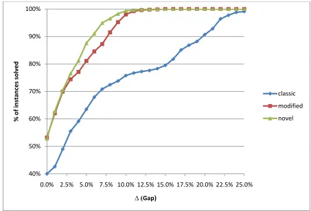
Table 5 presents the descriptive gap statistics, not including the instances that are solved to optimality, i.e., excluding those for which  0. The column labeled ―count” indicates the number of instances that cannot be solved to optimality within the time limit of 1200 seconds. For example, when P60, 77 instances cannot be solved using the classic formulation. The average gap of these 77 instances is  2.3%.

50% 55% 60% 65% 70% 75% 80% 85% 90% 95% 100%

0 100 200 300 400 500 600 700 800 900 1000 1100 1200

%

o

f i

n

stan

ce

s so

lv

e

d

t

o

p

tim

al

ity

Computation Time (s)

classic

modified

(50)

35 Table 5 - Gap Summary, Single Machine, Uniform Processing Times

 (Gap)

P Count Mean Std. Error Max Count Mean Std. Error Max Count Mean Std. Error Max

60 77 2.3% 0.16% 5.6% 29 1.4% 0.14% 4.3% 7 0.9% 0.08% 1.1%

100 128 1.4% 0.10% 5.6% 69 0.8% 0.04% 1.8% 15 0.5% 0.04% 0.8%

140 165 1.1% 0.07% 5.4% 125 0.7% 0.03% 2.7% 33 0.4% 0.04% 1.2%

As shown in Table 5, the gap performance of the classical formulation is the worst among these three formulations. Especially as the problem size increases, the novel formulation solves more instances to optimality compared to other two.

(51)

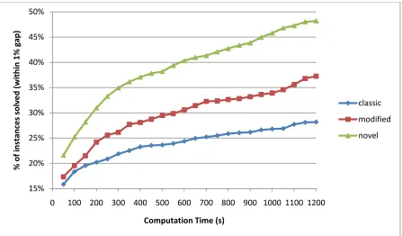
36 Figure 10 - Gap Performance, Single Machine, Uniform Distribution (Cumulative)

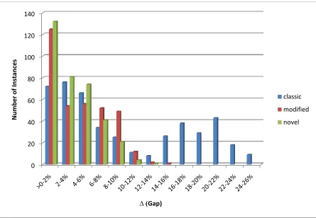
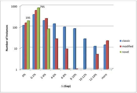
Figure 11 - Gap Distribution, Single Machine, Uniform Processing Times

65% 70% 75% 80% 85% 90% 95% 100%

0.0% 0.5% 1.0% 1.5% 2.0% 2.5% 3.0% 3.5% 4.0% 4.5% 5.0%

% o f i n stan ce s so lv e d Δ (Gap) classic modified novel 0 20 40 60 80 100 120 140 N u m b e r o f In stan ce s

∆ (Gap)

classic

modified

(52)

37 Both figures confirm the conclusion that the classic formulation performs the worst and the novel formulation performs the best among these three formulations. The performance of the modified formulation and the novel formulation does not differ by much when the total number of products is low. However, as the total number of products increases the novel formulation starts to outperform the modified formulation.

2.4.2 Experiment with the Mixed Processing Times

In the previous experiment, we generated all processing times from a single, relatively tight uniform distribution. Because of the “knapsack characteristics” of the problem, that kind of test bed is challenging and academically interesting. However, in real-life there are different customer types and related order sizes (small vs. large). We know that the 80-20 rule applies in many situations in practice, and indeed, data from our motivating problem indicates that approximately 15% of the orders are much larger than the remaining orders. To test the effect of this demand structure, in this experiment we generate the processing times from a mixture of distributions. The job-size index  is defined as follows:

1 if the job is small 2 if the job is big 

   

,

u p pt

t d  represents the processing type of a job. We sample the ―small jobs‖, ,1

u p pt

t d , from

[100, 200]

U

and we arbitrarily define the distribution for the ―big jobs‖ , t du_p _pt_,2, to be

[1000,1200]

U

_{since specific data from the motivating example is difficult to obtain, based on}

(53)

38 2.4.2.1Sample Instance Generation (Mixture Distribution)

We define a new parameter  (0  1) representing the percentage of products with high demand. In this experiment 0.15, meaning that only 15% of the products are in the high demand category.

The following algorithm is used to generate problem instances:

STEP 1: Generate a T by P matrix with random numbers

U

[0,1]

in each cell.

STEP 2: If the random number in a cell is greater than  , then set the cell value equal to 0 and go to step 3, otherwise generate a random number



from

U

[0,1]

. If



_{is greater than}, then  1, and generate the processing time from

U

[100, 200]

; else,  2generate the processing time from

U

[1000,1200]

.

STEP 3:



(1 ) [ ,1] [ ,2] [ ]



, 1

u u s

p pt p pt p

t

P E t d E t d E t

C    t



  

 



For our experiments, ts_p is fixed and ts_p ts, pmeaning that E t[ ]_ps ts. Also t du_p _pt_,1

is uniformly distributed between 100 and 200 implying that E t d[ up pt_,1] 150 . Similarly,

,2

u p pt

t d is uniformly distributed between 1000 and 1200 meaning that [ u _,2] 1100 p pt

E t d  . Since

we set 0.15 in our experiment, (1) [E t d_pu _pt_,1]E t d[ u_p _pt_,2]292.5. Microsoft Excel

(54)

39 2.4.2.2Experimental Results

We have exactly the same experimental design as the previous experiment except the processing times. Although only 15% of the products have high demand, it turns out that the problem gets significantly easier. Table 6 summarizes the mean and median computation times and the standard errors for different problem sizes. All formulations perform better with this demand structure compared to the previous experiment where a single uniform distribution was used. The mean computation times of the classic formulation are approximately the half of those from the previous experiment, while the mean computation times of the modified and the novel formulation are approximately one fifth of those from the previous experiment. That means all formulations perform better but the extent of improvement is much greater for the modified and novel formulations.

Table 6 - Computation Time Summary, Single Machine, Mixed Processing Times Time (s)

Classic Formulation Modified Formulation Novel Formulation P Mean Std. Error Median Mean Std. Error Median Mean Std. Error Median

60 136 19 2 26 8 1 6 3 1

100 241 25 4 51 12 3 9 4 1

(55)

40 Figure 12 - Average Computation Times vs. Problem size, Single Machine, Mixture

Distribution

As shown in Figure 12, there is only a small difference in performance between the modified formulation and the novel formulation when the problem size is moderate. However, as the total number of products increases, the novel formulation starts to outperform the modified formulation, similar to the experiment in the previous section.

Table 7 - Gap Summary, Single Machine, Mixed Processing Times ∆ (Gap)

P Count Mean Std. Error Max Count Mean Std. Error Max Count Mean Std. Error Max

60 46 1.7% 0.2% 6.2% 27 1.2% 0.1% 2.0% 0 0.0% 0.0% 0.0%

100 66 1.5% 0.1% 4.5% 13 0.7% 0.1% 1.9% 1 0.7% 0.0% 0.7%

140 78 1.0% 0.1% 3.5% 31 0.7% 0.1% 1.7% 6 0.4% 0.0% 0.6%

0 50 100 150 200 250 300 350

60 100 140

Co

m

p

u

tat

io

n

Ti

m

e

(

s)

Number of Products

classic

modified

(56)

41 Although the problem gets easier as the high demand products are introduced there are still some instances that cannot be solved to optimality by the classical and modified formulations. Only 7 instances out of 1080 cannot be solved to optimality using the novel formulation. Table7 summarizes those instances. Similar to the computation time results, all formulations perform better in terms of the remaining gap between the upper-bound and the lower-bound but the performance improvements in the modified and the novel formulation are much more noticeable than the improvement in the classical formulation. Please note that the maximum gap is never more than 2% in the modified formulation. The maximum gap resulting from the novel formulations is only 0.7%.

(57)

42 Figure 13 - Computation Time Performance, Single Machine, Mixture Distribution

(Cumulative)

Figure 14 - Gap Performance, Single Machine, Mixture Distribution (Cumulative)

70% 75% 80% 85% 90% 95% 100%

0 200 400 600 800 1000 1200

% o f in stan ce s so lv e d t o o p tim al ity

Computation Time (s)

classic modified novel 80% 85% 90% 95% 100%

0.0% 1.0% 2.0% 3.0% 4.0%

% o f In stan ce s solv e d

∆ (Gap)

classic

modified

(58)

43 Figure 15 - Gap Distribution, Single Machine, Mixture Distribution

The second computational experiment with the mixed demand distribution shows that the problem becomes easier if a small portion of the products have higher demand compared to the others. This is mainly because of the “knapsack characteristic” of the problem. Most of the time big jobs can be eliminated from current consideration in the branch and bound tree more easily compared to the smaller jobs. Specifically, in the branch and bound tree, big jobs are more likely to be eliminated from current consideration compared to the smaller jobs (i.e., their branches in the tree are more likely to be fathomed).

0 10 20 30 40 50 60 70

N

u

m

b

e

r

o

f In

stan

ce

s

∆ (Gap)

classic

modified

(59)

44

2.5 Comparison of the Formulations

In this section, we address the question of why there is a performance difference between three formulations. We first compare the classical formulation with the modified formulation and then the modified formulation with the novel formulation.

2.5.1 Classical Formulation vs. Modified Formulation

The main difference between the classical formulation and the modified formulation is the setup variable _pt and the production variable '_pt. In the classical formulation, the

variable _pt indicates whether the machine is set up for product p in period t or not.

However, the variable '_pt in the modified formulation only indicates whether product p is

produced in period t or not. Figure 3 and Figure 4 in Section 2.2 show this fundamental difference visually.

Mathematically, the relationship between these two variables can be represented as follows: '_pt _pt _{p t}_,_₁. Using this variable redefinition, the classical formulation can be

converted to the modified formulation. See Appendix A for further details. It turns out that this simple variable redefinition simplifies the branch and bound tree significantly.

Let’s assume that we have a single product and we are at some point in the branch

and bound tree. Since we have only one product we can drop the product index p for

convenience. We will branch on _t, _t_₁, _t and _t_₁ (or  '_t, '_t_₁, _t and _t_₁). Figure 16

(60)

45 labeled ―Inf”, represent the infeasible solutions. Note that this portion of the branch and

bound tree for the classical formulation has 26 nodes in total, while the portion of the tree for the modified formulation has 24 nodes in total. If we look at the trees carefully, we see that

they are the same except where _t 1, _t_₁0 and _t 1. This part of the tree is pruned by

infeasibility in the modified formulation because constraint (15) is violated when '_t 1,

1 '_t 0

   and t 1. More clearly, if we substitute the values of the variables into the

constraint 2_pt_{p t}_,_₁'_pt'_{p t}_,_₁0 we get 1_{p t}_,_₁0, which is always false.

(61)

46 Figure 16 - Branch & Bound Tree of the Classical Formulation

Figure 17 - Branch & Bound Tree of the Modified Formulation

γt=0

γt+1=0

ζt=0

ζ_t+1=0 inf inf

γt+1=1

ζt=0

ζ_t+1=0 ζ_t+1=1 inf

γt=1

γt+1=0

ζt=0

ζ_t+1=0 inf

ζt=1

ζ_t+1=0 inf

γt+1=1

ζt=0

ζ_t+1=0 ζ_t+1=1

ζt=1

ζ_t+1=0 inf

γ't=0

γ'_t+1=0

ζ_t=0

ζ_t+1=0 inf

inf

γ't+1=1

ζ_t=0

ζ_t+1=0 ζ_t+1=1 inf

γ't=1

γ'_t+1=0

ζ_t=0

ζ_t+1=0 inf

inf

γ'_t+1=1

ζ_t=0

ζ_t+1=0 ζ_t+1=1

ζ_t=1

ζ_t+1=0 inf

A Novel Solution Approach to Capacitated Lot-Sizing Problems with Setup Times and Setup Carry-Over.

Table of Contents

CHAPTER 1

1

INTRODUCTION

1.1 Literature Review

1.2 Problem Overview

1.3 Problem Notation and Properties





[0

 



1]











CHAPTER 2

2

SINGLE-MACHINE FORMULATIONS

WITHOUT HOLDING COST

2.1 Classical Restricted Capacitated Lot-Sizing Problem (CRCLSP)





 

t T



 

t T

2.2 Modified Restricted CLSP (Capacitated Lot-Sizing Problem)



 

t T









 

t T



 

t T

2.3 Novel Formulation







 

t T







t T







2.4 Computational Experiments







U

[100, 200]

U

[100, 200]





U

[0,1]

U

[100, 200]





[100, 200]

U

[1000,1200]

U

U

[0,1]



_{ }

_{t T}

_{ }

_{t T}

_{ }

_{t T}

_{ }

_{t T}

_{ }

_{t T}

_{t T}

_