Predictive Microstructural Modeling of Grain-boundary Interactions and Their Effects on Overall Crystalline Behavior

(1)

ABSTRACT

SHI, JIBIN. Predictive Microstructural Modeling of Grain-Boundary Interactions and Their Effects on Overall Crystalline Behavior. (Under the direction of Professor Mohammed A. Zikry.)

(2)

(3)

(4)

Predictive Microstructural Modeling of Grain-boundary Interactions and Their

Effects on Overall Crystalline Behavior

by

Jibin Shi

A dissertation submitted to the Graduate Faculty of North Carolina State University

in partial fulfillment of the requirements for the Degree of

Doctor of Philosophy

Mechanical Engineering

Raleigh, North Carolina 2009

APPROVED BY:

_________________________ _________________________ Dr. Ron Scattergood Dr. Kara Peters

__________________________ _________________________

(5)

DEDICATION

(6)

BIOGRAPHY

(7)

ACKNOWLEDGEMENTS

I would like to express my deepest appreciation to my advisor, Dr. Mohammed Zikry for his support and guidance throughout my Ph.D. program. Without his patience, encouragement and advisory, the dissertation would be impossible. His insightful suggestion and inspiration not only helped me in my current research, but will also enlighten my future career path.

I would also like to offer my special thanks to my committee members, Dr. Ron Scattergood, Dr. Larry Silverberg, and Dr. Kara Peters for their willingness to be my committee members and their time to provide beneficial suggestions and comments.

Support from the Office of Naval Research through Grant N000140510097, is gratefully acknowledged. The computations were performed in the High Performance Computation (HPC) Center of North Carolina State University. The support and assistance from Dr. Gary Howell in HPC center are highly appreciated.

I would also like to express my sincere thanks to the fellows in the solid mechanics lab: Dr. Omid Rezvanian, Tarek Hatem, James Pearson, Khalil Khodary, William Lee, Pratheek Shanthraj and Siqi Xu. It has been a wonderful experience to communicate with you and learn from each other. Your friendship made my Ph.D. study exciting and memorable.

(8)

(9)

LIST OF TABLES

Table. 1.1. Slip-systems of f.c.c. Metals...15

Table. 2.1. Parameters for Raj and Ashby GBS Rate ...39

Table. 3.1. CSL GB Misorientations...67

Table. 3.2. Material Properties of Copper ...67

Table. 4.1. Misorientation of Random Low Angle GBs ...97

(12)

LIST OF FIGURES

(13)

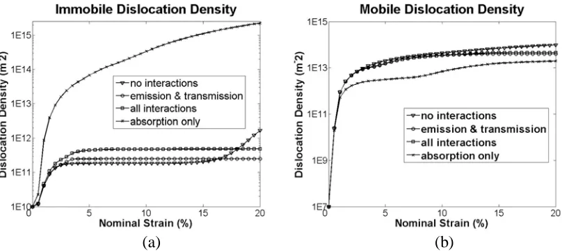
Fig. 3.7. Different GB interactions and dislocation-density behavior at 20% nominal strain: (a) semi-logarithmic plot of immobile dislocation-density development in one of the most active GB elements in the 17b bicrystal; (b) semi-logarithmic plot of mobile dislocation-density evolution in the neighboring element in 17b model. ...61 Fig. 3.8. Different GB interactions in most active element between GB and dislocation-densities of 17b model at 20% nominal strain: (a) the evolution of shear slip in an active GB element. (b) pressure in the same active GB element...62 Fig. 3.9. The nominal stress comparison for different schemes for the 17b bicrystal at 20% nominal strain. ...63 Fig. 3.10. The material behavior of the 1 bicrystal at 20% nominal strain: (a) the immobile dislocation-densities of the most active slip system 0 11

( )

111 without using the DDGBI scheme; (b) the immobile dislocation-densities of the most active slip system 0 11

( )

111 using the DDGBI scheme; (c) the resolved shear stress of the most active slip system

0 11

( )

111 without the DDGBI scheme; (d) resolved shear stress of the most active slip system 0 11

( )

111 with the DDGBI scheme; (e) Von Mises stress without using the DDGBI scheme; (f) Von Mises stress with the DDGBI scheme...64 Fig. 3.11. The behavior of the 3 bicrystal at 20% nominal strain: (a) the immobile dislocation-densities of the most active slip system 0 11

( )

111 without the DDGBI scheme; (b) the immobile dislocation-densities of the most active slip system 0 11

( )

111 using DDGBI scheme; (c) the resolved shear stress of the most active slip system 0 11

( )

111 without the DDGBI scheme; (d) resolved shear stress of the most active slip system

0 11

( )

111 with the DDGBI scheme; (e) Von Mises stress without the DDGBI scheme; (f) Von Mises stress with the DDGBI scheme. ...65 Fig. 3.12. The behavior of the 17b bicrystal at 20% nominal strain: (a) the immobile dislocation-densities of the most active slip system 011

( )

1 11 without the DDGBI scheme; (b) the immobile dislocation-densities of the most active slip system 011

( )

1 11 using DDGBI scheme; (c) the resolved shear stress of the most active slip system 011

( )

1 11 without the DDGBI scheme; (d) resolved shear stress of the most active slip system

(14)

(15)

(16)

(17)

011

(18)

CHAPTER 1 INTRODUCTION

1.1. GB Effects and GB Misorientations

(19)

(Hall 1951; Petch 1953). In contrast, for nano crystalline materials, grain boundary sliding (GBS) dominates the plastic deformation and significantly decreases the yield stress (Raj and Ashby 1971; Meyers, Mishra et al. 2006). In order to successfully model the mechanical properties of crystalline materials, it is crucial to have thorough understanding on GB behavior and interactions at different scales.

Desired material properties of most crystalline materials can be potentially obtained

by controlling the micro-structural aspects of GB behavior. The mechanical, physical and

chemical properties of the GBs can be optimized as a function of the spatial orientation and

the crystallography of each grain. The most common method that correlates the structures

and properties of GBs is the coincident site lattice (CSL) method (Randle 1993). In the CSL

formalism, certain orientations in space of two neighboring crystal lattices will result in a

periodic arrangement of the interfacing lattices. The CSL method provides a broad class of

GBs with different misorientations that can be used to investigate GB behavior. So for

example, 1 is a low angle CSL GB, and various experiments have indicated that dislocation

transmission can easily occur, and that there are no dislocation pile-ups in the GB region for

this CSL GB (Lee, Robertson et al. 1989; Lin and Pope 1993; Zhang, Wang et al. 2003;

Ohmura T 2004). 3 GBs are another type of CSL with slightly higher energy than 1 CSLs.

Experiments and simulations have shown that one of interactions between dislocations and

GBs for face centered cubic (f.c.c.) systems with 3 GBs is GB dislocation absorption

(Tanaka, Tsurekawa et al. 1994; Poulat, Decamps et al. 1998; Lucadamo and Medlin 2002;

(20)

absorption could be due to lattice dislocations dissociating into Shockley partial dislocations

in the GB region. Dislocation transmission (Lee, Robertson et al. 1990; Poulat, Decamps et

al. 1998) has also been widely observed for 3 GBs. For higher angle CSLs, such as, 5, 7,

17, and 19, in which there are no coplanar slip systems, dislocations can pile-up in the

GB, resulting in intergranular cracks (Lin and Pope 1995; Zikry and Kao 1996; Su, Demura

et al. 2002; Kameda, Zikry et al. 2006). The CSL method can correlates GB geometry and its

properties, but this pure geometrical GB description does not provide enough information to

predict and estimate special GB properties, other information such as GB structure, chemical

and electrical bonding (Sutton and Balluffi 1987) and local interactions between dislocations

and GBs is also important in determine the GB properties. Moreover, the CSL method is not

able to account for properties of random GBs if they do not fall into any CSL category

(Sutton and Balluffi 1987; Priester 1989). For random low angle GBs, in which

misorientations are generally less than 15°, GB dislocation (GBD) networks are usually well

organized with periodic patterns, and the GB energy is basically linearly proportional to the

misorientation angle (Read and Shockley 1950). Slip systems on each side of the GB are

nearly coplanar, which provide an easy path for dislocation transmission between grains. For

random high angle GBs, where misorientations are generally greater than 15°, the GBD

networks are usually thick and irregular, and the GB energy is usually much higher than

random low angle GBs, and the GB behavior is unpredictable due to the complexity of GBD

networks (Read and Shockley 1950; Watanabe, Yoshida et al. 1999; Amouyal, Rabikin et al.

(21)

1.2. Representation of GB Geometry and Coordinate Transformation

To define a geometrical description of a GB, the first step is to define its degrees of

freedom. As noted by Randle (Randle 1993), A GB in a bicrystal has eight degrees of freedom

in total: five of these are known as macroscopic and the other three microscopic (Goux 1974).

The macroscopic degrees of freedom of a GB characterize the geometry which relates the

overall orientation change occurring across the GB plane in a bicrystal. This definition

emphasizes the crystallographic nature of GB geometry and refers to the orientation

relationship (misorientation) across the surface of the GB. Of the five macroscopic degrees of

freedom, four define two directions (two each) and one defines an angle. The identity of the two

directions and angle depends upon whether the interface-plane scheme or the misorientation

scheme is used to describe the GB geometry. The surface of the GB is referred to as the GB

plane even though in reality it may not always be planar. The orientation of each grain is defined

by the orientation of its crystal coordinate system 100, 010, 001 with respect to a fixed reference

system.

In the interface-plane scheme, the five degree of freedom are two from the GB plane

normal (N1, N2) in each of the two grains and one () from the twist angle. It is pertinent

because it focuses on the concept of a GB as a joining together of two surfaces, followed in

general by a twist rotation, to forma bicrystal.

The second interpretation of the GB degrees of freedom starts from the relative rotation

between the orientations of the two neighboring lattices and is called angle/axis notation. The

angle/axis notation is more general and more commonly used. Different from the

interface-plane scheme, the angle/axis notation only define three degrees of freedom as it only represents

the relationship between the two neighboring lattices and not the position of the GB itself.

(22)

rotation axis (UVW) and one degree of freedom on rotation angle (). The macroscopic

definition of a GB is complete if one of the two GB normals (N1 or N2) is defined, since each

GB normal takes two degrees of freedom.

The angle/axis notation is one way in which the misorientation geometry of a GB may be

described mathematically; there is another equivalent description which use Euler angles (Bunge

1987). The orientation of each crystal is given by three Euler angles, 1, , 2, and the

orientation of the GB is given by a normal vector to the GB normal (N1 or N2). Therefore, these

five degrees of freedom will be sufficiently representative for planar deformation.

In the Bunge system (Randle 1993), the global crystallographic axes

(

[

100

]

,

[

010

]

,

[

001

]

)

are designated as (x2, y2, z2), and the local rotated axes are designated (x1,

y1, z1). Three successive rotations, based on specified Euler angles, are needed to represent the

crystallographic orientation of each grain. The three rotations are as follows:

Rotation m1: rotate about z1 by 1, so that the rotated x1 '

lies in the plane (x1,x2).

The rotated system now is (x1 '

, y2 '

, z2 '

).

Rotation m2: rotate about x1 '

by so that the rotated z1 "

is parallel to z2. The rotated

system now is (x1 "

, y1 "

, z1 "

).

Rotation m3: rotate about z1 "

=z2 by 2, so that the rotated x1 '''

and y1 '''

coincide with x2 and

y2, respectively.

The mathematical representations of Euler rotations are:

1 1

1 1 1

cos sin 0

sin cos 0

0 0 1

(23)

2

1 0 0

0 cos sin

0 sin cos

m =

, (1.1b)

2 2

3 2 2

cos sin 0

sin cos 0

0 0 1

m =

. (1.1c)

For two adjacent grains, misorienting one with respect to the other is performed by rotating each

crystal coordinate system by a transformation matrix, based on each crystal’s Euler angles, with

respect to a global polycrystal frame-of-reference. The misorientation transformation matrix for

Euler angles (1, , 2), is calculated by matrix multiplication of the rotation matrices

(

m m m 1, 2, 3

)

3 2 1

M =m m m . (1.2)

Using Eqns. (1.1) together with Eqn. (1.2) will yield

1 2 1 2 1 2 1 2 2

1 1

cos cos sin sin cos sin cos cos sin cos sin sin

cos sin sin cos cos sin sin cos cos cos cos sin

sin sin cos sin cos

M + = + _, (1.3)

which is the misorientation-transformation matrix expressed in terms of Euler angles.

Dislocation glide occurs in definite crystallographic planes and directions. The

combination of a particular slip plane and a slip direction in that plane is a slip-system. Face

centered cubic (f.c.c.) crystals deform on the close-packed octahedral

{

111

}

planes in the

<110> close-packed directions. There are four planes with three different slip directions,

therefore there are total of twelve slip-systems for each crystal. Hence, the two vectors

(24)

slip vector s.

The following transformation law for first-order Cartesian tensors defines the rotational

slip system in each crystal

'

ij ij

n =Mn , (1.4a)

'

ij ij

s =Ms . (1.4b)

The slip normal to and the slip direction vectors are given in the Table 1.1.

1.3. Intergranular and Transgranular Cracks

The intrinsic characteristics of GB structure, misorientations and interactions with

dislocations are essential microstructural factors in characterizing intergranular and

transgranular cracks. The transmission, absorption, emission or pile-up of dislocations will

have different effects on failure evolution and crack growth at the GB region. It has been

well-known by the pioneering work (Hanada, Ogura et al. 1986; Lin and Pope 1995) that low

angle GB and symmetrical 3 twin boundaries are particularly resistant to intergranular

crack. In contrast, most other CSL boundaries and high angle GBs were found to be prone to

intergranular crack (Zhang, Wang et al. 2003; Zhong, Xiao et al. 2006).

For low angle and 3 GBs, there are usually several coplanar or nearly coplanar slip

systems between two neighboring grains and dislocations can transmit between neighboring

grains without difficulty. The transmission of dislocations through these GBs attenuate the

stress in the GB region and prevent the formation of dislocation pile-up, hence intergranular

(25)

that when a random low angle GBs are ahead of a growing crack, the dislocations emitted

from the crack can easily transmit through the GB region into neighboring grain, and the

crack can penetrate the GB region without significant changes in the original crack

orientation (Zhang, Wang et al. 2003; Zhong, Xiao et al. 2006; Zhang and Wang 2008).

Computational simulations have also predicted the fracture toughness of low angle GB

(Gertsman and Tangri 1997; Kim, Hong et al. 2003) and successfully predict transgranular

crack based on the dislocation activities near the low angle GB region (Kameda and Zikry

1998).

In contrast, random high angle GBs are highly disordered usually with high

misorientation and interfacial energies (Shih and Li 1975; Watanabe, Yoshida et al. 1999;

Amouyal, Rabikin et al. 2005). There are no coplanar slip systems between most high angle

GBs and CSL GBs other than 3 and 1. The high misorientation, high GB energy and

complex GBD networks in high angle GBs usually result in dislocation absorption and

pile-ups in the GB region. These random high angle GBs act as strong barriers of dislocation

movement, and consequently change the original crack directions, and even render

transgranular cracks into intergranular cracks. There have been a lot of TEM experiments and

observations showing how high angle GB affects crack behavior. Robertson et al. observed

that a transgranular crack become intergranular after micro-crack initiates at the pile-up

region in high angle GB (Robertson, Lee et al. 1992); Zhong, et al. found that a transgranular

crack significantly changed its direction at a high angle GB (Zhong, Xiao et al. 2006); Zhang

(26)

severe dislocation pile-ups (Zhang, Wang et al. 2003; Zhang and Wang 2008).

Computational simulations are also coincident with about observations. Using MD method,

Farkas et al. have confirmed that transgranular crack can turn into intergranular cracks at

high angle GB (Farkas, Van Swygenhoven et al. 2002). Kemeda et al. successfully predict

intergranular cracks using dislocation-density based crystal plasticity and FE method

(Kameda and Zikry 1998).

1.4. Grain Size Effect and Hall-Petch Relation

It is well known that the mechanical properties, especially the yield strength, of crystalline materials are closely related to the grain size. Usually the smaller grain size corresponds to higher yield stress in crystalline materials. This fact is called Hall-Petch relationship (Hall 1951; Petch 1953) and it is

y =o+kd 1/2

. (1.5)

(27)

size and finally it reaches a lowest limit corresponding to the yield stress of amorphous materials (Nieh and Wadsworth 1991; Schuh, Nieh et al. 2002). However, there have been doubts on the inverse Hall-Petch relation and further investigations are needed to confirm it.

GBs play a critical role in the yield stress of materials in that there can be several

different deformation modes associated with different grain sizes, grain shape, temperature,

stress state and GB structures (Meyers, Mishra et al. 2006). There are four major deformation

modes for crystalline materials: 1. grain boundary sliding (GBS) caused by the atomic

shuffling of the GB interface; 2. collective GB migration; 3. stacking faults; 4. dislocations

from the interface to the grains (Sansoz and Molinari 2005). The first two modes correspond

to GB-mediated deformation and the last two modes correspond to dislocation-mediated

deformation. These deformation modes work together to finally determine the overall plastic

behavior and yield stress of crystalline materials.

For coarse grain materials, where Hall-Petch relation holds, the plastic deformation is

mainly attributed to dislocation-mediated deformation such as full and partial dislocations

evolution and annihilations, in which GBs act as barriers of dislocations movement, sinks

and sources of dislocations. GBS and GB migration are usually negligible and only occur

under certain conditions such as high temperature, high stress with long loading durations.

For crystalline materials with grain sizes of several nanometers, where inverse Hall-Petch

relation holds, plastic deformation is mainly attributed to the GB-mediated deformation, such

as GBS and GB migration. The GB-mediated deformation is considered as thermally

activated process that will reduce the yield stress of the nano-crystalline material according

(28)

migration. For example, Von Swygenhoven et al. found no contribution of grain interior in

total deformation of the MD model with average grain size of 5 nm (Van Swygenhoven and

Caro 1998).

1.5. Grain Boundary Sliding (GBS)

There are two different types of GBS. The first one is called Rachinger sliding (Rachinger 1952), which refers to the relative displacement of adjacent grains where the grains retain their original shape but displaced with respect to each other. Because oftentimes the polycrystals have irregular shape, the Rachinger sliding usually have to be accommodated by some intragranular movement of dislocations within the adjacent grains. The other type of sliding is called Lifshitz Sliding (Lifshitz 1963), which refers to the boundary offsets that develop as a direct consequence of the stress-directed diffusion of vacancies. The above types of sliding are results of thermal activation process, such as diffusion and atom shuffling, but some of MD simulations (Van Swygenhoven and Caro 1998; Sansoz and Molinari 2005) indicate that GB sliding may also happen at 0K, which indicates that the GBS also contains an athermal component.

(29)

both GB and bulk diffusion into consideration, Fu et al. (Fu, Benson et al. 2004)obtained expressions on GBS rate on different grain shapes.

1.6. Experimental and Computational Methods

There are many methods to study the mechanical properties of materials, experimental test, molecular dynamics simulation and finite element methods are the most frequently used methods. Conventional microscopy, scanning electron microscopy (SEM) , X-Ray topography and transmission electron microscopy (TEM) are widely used to observe underlying micro-scale interactions and mechanisms, among which, TEM is by far the most important technique for studying defects in great detail. TEM is a microscopy technique whereby a beam of electrons is transmitted through an ultra thin specimen, interacting with the specimen as they pass through. An image is formed from the interaction of the electrons transmitted through the specimen, which is magnified and focused onto an imaging device. There have been a lot of TEM observations on detailed physical mechanisms of dislocations, especially interactions between dislocations and GBs (Robertson, Lee et al. 1989; Lee, Robertson et al. 1992; Hu, Molodov et al. 2000). In order to observe dynamic behavior of nano-crystalline materials, In-situ TEM technique has been widely used (Lagow BW 2001; Gemperlova J 2002; Ohmura, Minor et al. 2005).

(30)

method provides insights that may be not possible with TEM in-situ observations on the nano scale. The MD methods have shown that GBs can act as sinks and sources of dislocations (Schiotz 2004; Van Swygenhoven, Derlet et al. 2006). Dislocations can be absorbed in the GB causing pile-ups (Yamakov, Wolf et al. 2003; Schiotz 2004) and cross-slip (Yamakov, Wolf et al. 2003). But, severe limitations on time and length scales may render these simulations ineffective on the micro-structural physical scale that pertains to the inelastic behavior of crystalline aggregates.

(31)

(32)

Table. 1.1. Slip-systems of f.c.c. Metals Slip system # Slip system

1

( )

111 01 1

2

( )

111 101

(33)

CHAPTER 2 FORMULATIONS

In this chapter, the formulations used in the modeling of different GB behavior are presented, which includes dislocation-density based multiple-slip crystal plasticity constitutive formulation, the GB dislocation-density interaction scheme, the misorientation dependence on initial GB dislocation-densities, and Raj-Ashby GBS formulation.

2.1. Dislocation-density Based Multiple-slip Crystal Plasticity Constitutive

Formulation

The formulation for the multiple-slip crystal plasticity rate-dependent constitutive relations, and the derivation of the evolutionary equations for the mobile and immobile dislocation-densities, which are coupled to the multiple-slip crystalline formulation, are presented in this section. The detailed presentation of this constitutive formulation is given by Zikry and Kao (Zikry and Kao 1995).

2.1.1.

Multiple-slip Crystal Plasticity Constitutive Formulation

It is assumed that the deformation gradient can be decomposed into elastic and plastic components. The velocity gradient tensor, Vi,j is related to the deformation gradient by

1 ,

i j ik kj

(34)

where Fij is the total deformation gradient. The velocity gradient, Vi,j, can be decomposed

into symmetric and anti-symmetric parts as

V_ij=D_ij+W_ij, (2.2)

where Dij is symmetric part, representing the deformation rate tensor, and

(

, ,

)

1 2

ij i j j i

D = V +V . (2.3)

Wijis the anti-symmetric part, representing the spin tensor, and

(

, ,

)

1 2

ij i j j i

W = V V , (2.4)

It is assumed that the spin tensor Wij and deformation rate tensor Dij can be further

decomposed into elastic and plastic components as

Dij =Dij p₊

Dij

*

, (2.5)

W_ij=W_ijp₊ W_ij*

. (2.6)

The superscript * means that the elastic part and the superscripts p denotes the plastic

part. Wij *

represents the rigid body spin. The elastic components of the velocity gradient Dij

*

correspond to the elastic lattice distortion and the inelastic parts are defined in terms of the

crystallographic slip rates as

( ) ( )

p ij ij

D =P , (2.7)

( ) ( )

p ij ij

(35)

where is summed over all slip systems and the tensors Pij ()

and ij ()

are symmetric and

skew-symmetric second-order tensors, and are defined in terms of the unit normals and the

unit slip vectors as

Pij

() ₌ 1

2 si

( )_n

j

( )₊_s

j

( )_n

i

( )

(

)

, (2.9)

ij

() ₌ 1 2 si

( )_n

j

( )_s

j

( )_n

i

( )

(

)

. (2.10)

where ni ()

is the unit vector normal to the slip plane, and si ()

is the unit vector in the slip

direction.

The elastic response can be expressed in terms of a hypoelastic law

*

ij L D_ijkl _kl

= , (2.12)

where Lijkl is the fourth-rank elasticity tensor with Voigt symmetry and

*

ij

is the Jaumann

rate of Cauchy stress, ij, co-rotational with the lattice spin.

The objective stress rate used here, is given by

*

* *

ij _ij W_ik _kl W_jk _kl

= , (2.13)

where ijis a material time-derivative of Cauchy stress.

The objective stress rate, ij

, co-rotational to the material element can be derived as

(

p

)

p p

ij L_ijkl D_kl D_kl W_ik _kj W_jk _ki

= , (2.14)

(36)

(

)

ijkl ik jl jk il ij kl

L =μ + + , (2.15)

where ij is the Kronecker delta and and μ are the Lamè constants.

For a rate dependent formulation, the slip-rates are functions of the resolved shear

stress and the reference shear stress on each slip-systems in a power law form of

( ) ( ) ( )

( )1/m 1

ref ref ref =

(no sum on ), (2.16)

where ref

( ) _{is the reference shear strain rate which corresponds to a reference shear}

stress ref

()_{, and}_m_{is the rate sensitivity parameter and}_m_{is given by}

( ) ( ) ln ln m =

. (2.17)

For most of the metals, m is close to 100 at room temperature when the shear slip rate is

smaller than a critical value and approximately equal to 1 when shear slip rate is greater than

the critical value. In this case, the flow is assumed to be characterized by drag-controlled

dislocation motion. The rate-independent limit is achieved as m approaches zero. For

multiple slip, is taken as the sum of the accumulated plastic strains on all slip systems n,

( ) 1 n =

=

, (2.18)

where ()_{is the resolved shear stress and is given in terms of the Cauchy stress by}

( ) ( )

ij ij

P

= (2.19)

From the balance of energy, with no thermal conduction, the time rate of change of

(37)

' p ij ij p T D c = _(2.20)

where is the fraction of the plastic work converted to heat, ij’

is the deviatoric stress, is

the material density, and cp is the specific heat of the material.

2.1.2.

Evolutionary Equations for the Mobile and Immobile Dislocation-densities

To gain a more fundamental understanding of dislocation motion, interaction, and

transmission on material failure modes, the crystal plasticity constitutive formulation is

coupled to internal variables that account for a local description of the dislocation structure in

each crystal. Specifically, the mobile and the immobile dislocation-densities have been used

as the internal variables in the present constitutive formulation. In inelastic deformations, the

characteristics of the microstructure are governed by the mechanisms of dislocation

production and dynamic recovery. As the material is strained, immobile dislocations are

stored in each crystal, and these dislocations act as obstacles for evolving mobile

dislocations. Therefore, the immobile and mobile dislocation-densities can be coupled, due to

the continuous immobilization of mobile dislocations.

The reference shear stress is a modification of widely accepted classical forms that

relate the reference shear stress to a square-root dependence on the immobilized

dislocation-density as ref ( )₌ y

( )₊_aGb

im

( )

=1 12

(38)

where b is the magnitude of burgers vector, G is the shear modulus, y ()

is the static yield

stress, and a is interaction coefficients, and generally have a magnitude of unity.

For a deformed material, it can be assumed that the dislocation structure of total

dislocation-density ()

can be additively decomposed into two components: immobile

dislocation-density im

()

and mobile dislocation-density m

()

as

( ) =m

( )₊

im

( )_. _(2.22a)

Following the approach of Gottstein et al. (Gottstein and Argon 1987), we assume

that during an increment of strain, the dislocation-density generates (denoted by()+_{) and}

annihilates (denoted by (

)-) on each slip system as

( ) ( ) ( ) im im im d dt ₌ +₊ (2.22b) ( ) ( ) ( ) m m m d dt ₌ +₊ (2.22c)

where im( )

+

and im( )

correspond to the generation and annihilation of immobile

dislocation-densities, and m( )

+

and m( )

correspond to the generation and annihilation of

mobile dislocation-densities.

The balance between dislocation generation and annihilation, Eqns. (2.22b-c), is the

basis for the evolution of mobile and immobile dislocation-densities as a function of strain.

Plastic deformation of the crystal is assumed to begin with the easy glide stage, stage I. In this

stage, most of the dislocations belong to the primary slip-system, and very little slip takes place

on secondary slip-systems. Also, dislocation-densities are comparatively low, and the details of

(39)

high-resolution methods. In the second stage of hardening (stage II), secondary slip systems are

activated, and dislocation clusters and cell walls begin to form. The third stage of hardening is

characterized by the annihilation and the rearrangement of dislocations. For a detailed

experimental overview of dislocation emission, interaction, trapping, and annihilation for the

three hardening stages in f.c.c. materials, see, for example, (Anongba, Bonneville et al. 1993;

Anongba, Bonneville et al. 1993; Argon and Haasen 1993).

In stage I, dipoles and multipoles are formed after mobile dislocations emitted from a

source are trapped by dislocations of opposite signs on parallel slip planes. The back stress at

the source is due to the dislocation emitted by the source. If the flow stress is greater than this

back stress, the source will continue to emit dislocations, and dislocations that are trapped can

break free. A large number of dipoles, multipoles, and loops are formed in easy glide by forest

interactions, cross-slip around obstacles, and interactions between dislocations on parallel slip

planes. Dipoles and multipoles occur in well-spaced clusters, thus allowing primary dislocations

to glide over long distances. Using the Eqn. (2.22c), this is given by

( ) m d dt ₌

rate of generation. (2.23)

The rate of dislocation generation is proportional to the distance traveled by the emitted

dislocations from a dislocation source with density souce( )

. This distance, yback, is related to the

decrease of the back stress on the dislocation-density source, souce( )

, after previously emitted

dislocations have traveled this distance yback. Hence, Eqn. (2.23) can be written as

( ) ( ) m source back d v dt y ₌

, (2.24)

where v is mobile dislocation average velocity. Using Orowan’s equation, ( ) m( )bv

and

(40)

( ) ( ) ( )

2

m sour im m d g d b =

, (2.25)

where b is the modulus of the Burgers vector, gsource is a coefficient pertaining to an increase in

the mobile dislocation-density due to dislocation sources.

In stage II, dipole clusters multiply and join together, so that primary glide dislocations are

efficiently blocked. Hardening increases in this stage are due to an increase in dislocation

tangles. The forest dislocations of these systems serve as obstacles for the primary dislocations.

The mobile dislocations are immobilized with a mean free path proportional to

( )

im( ) 1/ 2

.

Spatially organized forest structures and tangles such as Frank nets, cell walls, or

sub-boundaries can act as immobilization sites at this stage of the deformation. Also thermally

activated cross slip can block the glide dislocations. Since the rate of trapping is related to an

increase in rate of growth of immobile dislocations, using Eqn. (2.23), the coupled mobile and

immobile dislocation-density evolution equations for this stage are given by

( )

( ) min

2 exp ,

m immob ter im

d g g H

d b b kT

= (2.26)

( )

( ) min

2 exp ,

im immob ter im

d g g H

d b b kT

= + (2.27)

where b is the modulus of the Burgers vector, gimmob is a coefficient related to the immobilization

of mobile dislocations, and gminter is a coefficient related to the trapping of mobile dislocations

due to thermally activated cross-slip.

At moderate and large strains, dynamic recovery characterizes the stage III. At

temperatures lower than 40% of the melting temperature, the main mechanism of recovery is

annihilation of the screw segments of opposite signs on the expanding dislocation loops. The

(41)

( ) ( ) cov im re im d g d

= , (2.28)

where grecov is a coefficient related to the rearrangement and annihilation of immobile

dislocations.

Eqns. (2.25-2.28) can be combined to obtain a coupled set of nonlinear evolutionary equations

( )

( ) ( )

( ) min ( )

2 2 exp

m sour im ter immob im m

d g g H g

dt b b kT b

=

, (2.29)

( )

( ) min ( ) ( )

cov

2 exp exp

im ter immob

im re im

d g H g H

g

dt b kT b kT

₌ ₊

, (2.30)

where gsour is a coefficient pertaining to an increase in the mobile dislocation-density due to

dislocation sources; gminter is a coefficient related to the trapping of mobile dislocation due to

forest interactions; grecov is a coefficient related to the rearrangement and annihilation of

immobile dislocations; gimmob is a coefficient pertaining to the immobilization of mobile

dislocations; H is the activation enthalpy; and k is the Boltzmann’s constant. As these

evolutionary equations indicate, the dislocation activities related to recovery and trapping are

coupled to thermal activation. The thermal activation energy temperature is updated as a

function of the energy equation given by (2.20).

2.1.3.

Determination of the Coefficients for the Coupled Evolution Equations

To couple the evolutionary equations to the crystal plasticity formulations, the four g

coefficients in (2.29-2.30), and the enthalpy, H, must be determined as functions of the

(42)

current temperature to the reference temperature, following Paidar, Pope et al. (Paidar, Pope et al.

1984), a form of activation enthalpy for cross-slip which accounts the cross-slip effects. The

four g coefficients are determined using two general conditions, pertaining to the evolution of

dislocation-densities in crystalline materials, have been used:

(i) that the mobile and immobile dislocation-densities saturate at large strains;

(ii)that the relaxation of the mobile dislocation-density to a quasi-steady state value

occurs much faster than the variation of the immobile dislocation-density.

The conditions are invoked based on the arguments by Mecking and Kocks (Mecking and Kocks 1981), Walgraef and Aifantis(Walgraef and Aifantis 1985; Walgraef and Aifantis 1985; Walgraef and Aifantis 1985; Walgraef and Aifantis 1985), and Estrin and Kubin (Estrin and Kubin 1988; Kubin and Estrin 1988). They used similar arguments to determine coefficients in equations pertaining to the evolution of mobile and immobile dislocation-densities. The saturation of both the immobile and mobile dislocation-densities at large strains and the their to different quasi-steady values in f.c.c. materials have been experimentally substantiated by several investigators (see, for example, Mughrabi,(Mughrabi 1987); Hansen, (Hansen 1990)). For a detailed presentation, see to (Zikry and Kao 1996; Zikry and Kao 1996; Kameda and Zikry 1998).

2.2. Dislocation-density Grain Boundary Interaction (DDGBI) Scheme

In this section, a dislocation-density grain boundary interaction (DDGBI) scheme is

presented to account for the GB dislocation-density activities. It is assumed that the

(43)

Based on the single transmission criteria by Clark et al. (Clark, Wagoner et al. 1992), a

transmission criteria for multiple slip is proposed as follows:

Criteria 1. A transmission factor is proposed based on two components. The first one

is the angle (Fig. 2.1), which is the angle between the intersection lines of the slip planes

and GB planes; the second part is the angle between slip directions of these two slip

systems. Hence, the transmission factor M can be denoted as

M =cos cos, (2.31)

where =arccos(l l1 2) in which (l1=n n1 GB

and l2 =n n2 GB

), (2.32a)

and =arccos

(

s s1 2

)

, (2.32b)

Criteria 2. The ratio of resolved shear stress to the reference shear stress of the

outgoing slip system (stress ratio) should be greater than a critical value ccr, which is

approximately one.

If these transmission criteria are satisfied, a dislocation-density can emit from a

higher dislocation-density region to a lower dislocation-density region. It is assumed that the

dislocation-densities will be redistributed according to these transmission factors as shown in

Fig. 2.2. Based on this, a balance of densities due to these different

dislocation-density interactions, out ()

, can be defined as

out( ) ₌ M out ( )_/ ref ( )

(

)

Miout i ( ) _/ ref i ( )

(

)

i=1 m

inc

(44)

where is an incoming slip system, is an outgoing slip system, out() is the corresponding

resolved shear stress, and ref()_{is the reference shear stress of the outgoing slip system .}_m_is

the number of all possible outgoing slip systems, and M is the transmission factor between

the incoming and outgoing slip systems.

When dislocation-densities emit from one element to the other, a balance for the

dislocation-densities can be obtained by considering dislocation-density conservation

(Aifantis 1987).

( )

( ) ( ) ˆ

c div j t ₌

, (2.34a)

where ( )

( ) ( ) ndA ndA t t div j x y = +

, (2.34b)

where j( ) represents the flux of dislocation-densities in slip system , A is area of

integration, n is the GB surface normal, () is the summation of the dislocation-densities

changes in the domain indicated by Eqn. 2.33, and cˆ( ) represents the generation,

immobilization or annihilation of dislocations densities. cˆ( ) is given by the statistical

distribution of the immobile and mobile dislocation-densities from Eqns. 2.35a-b.

( ) ( ) min ( ) ( )

cov 2

ˆ ter exp immob exp

im im re im

g H g H

c g

b kT b kT

₌ ₊

, (2.35a)

( ) ( ) ( )

( ) min ( )

2 2

ˆ sour im ter exp immob

m im

m

g g H g

c

b b kT b

=

. (2.35b)

(45)

( )

( ) min ( ) ( )

cov

2 exp exp

im ter immob

im re im

d g H g H

g div j

dt b kT b kT

₌ ₊

, (2.36a)

( ) ( )

( ) min ( )

2 2 exp

m sour im ter immob im m

d g g H g

div j

dt b b kT b

=

. (2.36b)

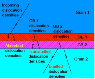
Dislocation-density activities can occur in the GB interface and at GB-interior interfaces (Fig. 2.1-2.2). In the proposed GB representation, we assume that dislocation-density transmission occurs when immobile dislocation-densities transmit through the GB interfaces

to compatible slip systems in the neighboring grain. Dislocation-density absorption occurs when mobile dislocation-densities from the grain interior transmit into the GB, but do not transmit out of it. In this case, all of the mobile dislocation-densities are then immobilized to immobile dislocation-densities, and are assumed to be absorbed in the GB. Some of these immobile dislocation-densities in the GB regions may pile-up, but as the deformation evolves can activate neighboring slip systems. This can result in dislocation-density emission, in which the immobile dislocation-densities in the GB become mobile dislocation-densities and emit into the neighboring grain. Hence, all three processes of transmission, absorption, and

emission can occur simultaneously on different slip-systems within the GB region and between neighboring grains.

2.3. Initial dislocation-densities dependence on GB misorientations

(46)

misorientation and initial dislocation-densities (before deformation) in low angle GBs. That relation is

x =

acos, (2.37a)

y

=

a

sin

, (2.37b)

where x and y are the line density of initial dislocation at x and y directions; is the tilt misorientation of the GB, a is the lattice parameter; is the angle between lattice and GB, and 0<</2. Assuming that the grain has a rectangular shape, and the grain size is d, the initial dislocation density due to GB misorientation can be given as

im = 2

d

(

x +y

)

=

2

ad

(

cos+sin

)

. (2.38)

According to this equation, the initial dislocation-density is grain size and misorientation dependent. This can be critical, since for nanocrystalline materials, the initial dislocation-densities in the GB region are usually higher than the grain interior (Read and Shockley 1950; Gleiter 1977; Van Swygenhoven, Farkas et al. 2000).

2.4. GBS mechanism

(47)

nodal velocity ut is a combination of dislocation-mediated deformation and GB-mediated deformation as

ut =udis +ugbs, (2.39)

where udisis the dislocation-mediated velocity and ugbsrepresents the GBS velocity. The GBS rate of nanocrystalline material is accounted for by the Raj and Ashby equation as

ugbs =

dugbs dt = 2 a kT

h2 DV 1+

DB

D_V

, (2.40)

where a is the shear stress along the direction of the GB, is the atom volume, is the wavelength, and h is the amplitude of the GB. DV and DB are volume and boundary diffusion coefficients, is the GB width, k is Boltzmann constant, and T is temperature. At temperature significantly below melting point, DB>>DV, and hence the Raj and Ashby equation can be given as (Fu, Benson et al. 2001; Kim, Hiraga et al. 2005)

ugbs =

2DBa

kT 1

h2 . (2.41)

(48)

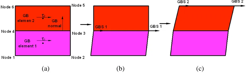
rate (ugbs) is calculated from Eqn. 2.41. The deformation mode of GBS is assumed to be simple shear along the tangential direction of the GB element. Assuming GBS only occurs in the GB elements, and the GBS at the interfacial nodes are given by simple shearing of the lower element (Fig. 2.3b), the GBS on the top nodes are given by the summation of the GBS of the interfacial nodes in element 1 and shear displacement of the top nodes in element 2 (Fig. 2.3c). The total nodal velocity can then be updated by the summation of dislocation-mediated displacement and GBS by Eqn. 2.39.

2.5. Computational Methods

To update the stress state of the crystalline material, both the total deformation rate

tensor, Dij, and the plastic deformation rate tensor, Dij p

, are needed. A brief outline of the

numerical method will be presented; for further details see Zikry (1994). An implicit finite

element method analysis has been used to obtain the total deformation rate tensor, Dij. The

displacements have been obtained by the quasi-Newton solution of the static-equilibrium

equation, with BFGS iteration to ensure convergence of the quasi-Newton method. Once the

displacements are obtained, the deformation tensor can be calculated. To overcome numerical

problems associated with incompressible displacements, the Bmethod has been used in the

calculation of the deformation tensor. In the B method, the deformation gradient is

decomposed into volumetric and deviatoric parts. The volumetric part of the deformation tensor

is then computed at reduced quadrature points. The resulting volumetric deformation field

eliminates spurious modes that can arise due to incompressible deformations. Once the

deformation tensor is obtained from the updated nodal displacement values, the total

(49)

To solve for the plastic deformation rate tensor, Dijp, the time derivative of the resolved shear stress

( )

(

( )

)

ij ij d P dt

= , (2.43)

is used together with the objective stress rate, and the assumption that the elastic modulus tensor

is isotropic, to obtain the following system of nonlinear differential equations for each active slip-system :

( ) ( ) *

ijkl ij kl

L P D

= , (2.44)

in expending form

( ) ( ) ( ) ( ) ( )

( )

1

2

m ij ij ij ref

ref

P D P

μ =

. (2.45)

It has also been assumed, in the derivation of Eqn. (2.45), that the lattice spin is a

function of the elastic spin in all three directions

( ) * ( )

i W sij j

s = , (2.46a)

( ) * ( )

i ij j

n =W n , (2.46b)

where the elastic lattice spin is obtained as

* p

ij ij ij

W =W W . (2.47)

The solution to the system of ordinary differential Eqn. (2.45) is numerically difficult,

not only due to the nonlinearity of the resolved shear stress, but also because the system of

equation is numerically stiff in certain time intervals. The different time scales pertaining to the

resolved shear stress on each slip-system cause the numerical stiffness. These results in

(50)

leads to the growth of numerically propagated error, i.e., instability in the solution of the system

of differential equations. The computational scheme developed by Zikry (1994) is used to solve

the system of Eqn. (2.45). This algorithm is also used to update the evolutionary equations for

the immobile and mobile dislocation-densities.

Since the system of equations given by Eqn. (2.45) is only stiff in some regions of the

integration domain, an explicit fifth-order accurate Runge-Kutta method is used over most of

the time domain. The propagated error is measured by the growth in the local truncation error.

If the time-step must be restricted due to stability and not accuracy, a backward Euler method is

used. The backward Euler method is both A-stable and stiffly stable; it is also an order one

Backward Differentiation Formula (BDF). The algorithm methodology is as follows:

Automatic step control has been achieved by using step doubling on the Runge-Kutta

fourth-order method. Two approximate solutions are taken, one solution of step size 2hand a

second solution with two steps, each of size h. Since the original method is fourth order, the two

numerical methods are related by

(

)

( )

5

( )

₆

1

ˆ

2 2

t h h O h

+ = + + +, (2.48)

(

)

( )

5

( )

₆

2

ˆ

2 2

t h h O h

+ = + + +, (2.49)

where is of the order 5

(t)/5!. Furthermore, the two numerical methods are combined to

give a solution of fifth-order accuracy

(

)

( )

6

2 ˆ 2

15

t h O h

+ = + + +, (2.50)

where is the local truncation error which measures how well the solution is approximated

(51)

0.20

1

o new old

h =Fh

(2.51)

where hnew is the adjusted time step, and holdis the initial time step. The actual accuracy, 1, is

measured by the supremum norm as max |1-2|, and o is the desired accuracy measured by H. Here is the tolerance level supplied by the user and H is a scaling factor for fractional

errors for the ith equation given by hd dt

+ , where h is the initial time step. The factor F

serves to keep the new time step small enough to be accepted if the truncation error in the next time step is growing. Based on Eqn. 2.51, the time step is increased if the truncation error is

smaller than the desired accuracy, and conversely the time step is decreased if the truncation

error is greater than the desired accuracy.

Since Runge-Kutta methods have finite stability regions, there can be a growth in the

propagated error and, therefore, the time step in certain time domains, can be restricted due to

stability and not accuracy requirement by H. This is an indication of stiff behavior. In the

present algorithm, the largest allowable time step is chosen, i.e., the time step on the stability

boundary. This implies that the local errors are of the same magnitude as the accuracy tolerance

used in Eqn. (2.45). If the time step is unduly restricted due to stability, the solution will

proceed in time, albeit inefficiently, due to the necessity of using intolerably small time steps. To correctly identify the regions of numerical stiffness, and to distinguish a step reduction due to accuracy from a time step reduction due to stability, a stiffness ratio, SR, has been defined as

max 2 1 min Re ₁ Re R S t t =

(52)

where |Re|max and |Re|min are the greatest and smallest absolute values of the real parts of the

eigenvalues of the Jacobian of the system of ordinary differential equations given by Eqn.

(2.45), and t2-t1 is the time interval of the integration. A large stiffness ratio, SR, indicates that

the ratios of the eigenvalues are dispersed relative to the time scale.

When the time step is restricted due to the presence of these widely varying eigenvalues,

this is a stability problem, and an indication that the initial value problem is numerically stiff. An

increasing stiffness ratio is an indication that for a specified deformation mode, the slip rate,( ) ,

are much greater for one slip-system than for the other active slip-systems; namely, one of the

slip-systems may be dominating the deformation process. The domination of one slip-system

over other active slip-systems can occur, for example, when a macroscopic shear ban is forming

in a crystalline solid (see, for example, Zikry, 1994 (Zikry 1994)).

If the stiffness ratio is increasing, then this is an indication of numerical stiffness, since

the time step is being reduced due to stability considerations. In the present analysis, when stiff

behavior is encountered, the integration is automatically switched to the backward Euler scheme.

The quasi-Newton method has been used to solve the system of nonlinear algebraic equations.

(53)

(54)

(55)

(a) (b) (c)

(56)

Table. 2.1. Parameters for Raj and Ashby GBS Rate

Properties k (JK-1) DB (m3) (nm) h (d)

(57)

CHAPTER 3 MODELING OF GRAIN BOUNDARY TRANSMISSION, EMISSION,

ABSORPTION AND OVERALL CRYSTALLINE BEHAVIOR IN

1,

3,

AND

17b BICRYSTALS

(58)

dislocation-density absorption, transmission and emission are interrelated interactions. These GB processes are directly related to microstructural behavior, and can be potentially controlled for desired material response.

3.1. Introduction

Grain boundaries (GBs) play a critical role in the mechanical properties of materials in that they can act as barriers or initiators of dislocation activities. Dislocations can be absorbed, piled-up, reflected, transmitted or emitted into or from GBs based on the crystallographic nature and the evolving local properties of the GBs and adjacent grain interiors. The dislocation structures in the GB are very different than those in the grain interior due to various types of partial dislocations and dislocation absorption and accumulation that can arise from GB misorientations (Gemperle, Gemperlova et al. 2002).

(59)

the outgoing slip system must be a maximum. These three criteria have been used to understand single dislocation transmissions and to rationalize multiple dislocation activities (Lee, Robertson et al. 1990; Gemperlova J 2002; Gemperlova, Polcarova et al. 2004).

Computational simulations have also provided insights of these GB activities on

different physical scales. Molecular dynamics (MD) simulations have shown that GBs can

act as sinks and sources of dislocations (Schiotz 2004; Van Swygenhoven, Derlet et al.

2006). Dislocations can be absorbed in the GB causing pile-ups (Yamakov, Wolf et al. 2003;

Schiotz 2004) and cross-slip (Yamakov, Wolf et al. 2003). These MD methods provide

insights that may not be possible with TEM in-situ observations on the nano scale. But,

severe limitations on time and length scales may render these simulations ineffective on the

micro-structural physical scale that pertains to the inelastic behavior of crystalline

aggregates.

Finite element models (FEM) and different crystalline plasticity formulations have

provided further insights on GB behavior. Ashmawi and Zikry (Ashmawi and Zikry 2003)

have introduced interfacial GB regions to track slip and dislocation-density transmissions and

intersections for a formulation based on dislocation-density based crystalline plasticity. Other

investigators (de Koning, Miller et al. 2002; de Koning, Kurtz et al. 2003; Dewald and Curtin

2007) have coupled FEM with MD formulations for a multi-scale approach.

(60)

(61)

neighboring grains in 3 GBs. In these results, by the aid of weak beam TEM, residual dislocations were found to be absorbed in the GB. MD simulations of a 3 GB (Spearot, Jacob et al. 2007) indicate that the GB can also act as source of dislocation nucleation. There were no observable pile-ups in crystalline materials with 3 GBs. For higher angle CSLs, such as, 5, 7, 17, and 19, in which there are no coplanar slip systems, dislocations can pile-up in the GB, resulting in intergranular cracks (Lin and Pope 1995; Zikry and Kao 1996; Su, Demura et al. 2002; Kameda, Zikry et al. 2006).

Hence, it is essential to understand and to predict how different CSL orientations affect behavior at the relevant scale. In this paper, a methodology based on a multiple slip dislocation-density crystalline formulation and specialized finite-element approaches is introduced to predict GB behavior. This approach is used to model and understand the behavior of bicrystals with a representative class of CSL boundaries that span different orientations.

(62)

3.2. Results and Discussions

The multiple-slip crystal plasticity dislocation-density based constitutive formulation and the FE computational scheme are used to investigate material deformation mechanisms associated with low and high angle CSL boundaries in f.c.c. crystalline copper bicrystals. The 1, 3, and the 17b CSL GB orientations were chosen to study the deformation modes and

failure mechanisms in materials separated by these CSL boundaries. These CSL GBs were chosen because they span a wide range of GB orientations in crystalline materials. The 17b CSL GB has one of the largest angles of misorientation about the tilt axis, 86.63°, and the 1 CSL GB has one of the smallest misorientations of less than 15° (Randle 1993). The misorientations of these CSL GBs are given by Table. 3.1.

The material properties that are used here (Table. 3.2) are representative of crystalline copper (see, for example, (Zikry 1994)). The initial immobile dislocation-density, ims, was chosen as 1010 m-2, and the initial mobile dislocation-density ms, was chosen as 107 m-2. The values of the initial and the saturated dislocation-densities are representative of copper (Mughrabi 1987). Based on the scheme developed by Zikry and Kao (Zikry and Kao 1996), we have obtained the coefficient values needed for the evolution of the immobile and mobile densities and the specified material properties. These values are gminter = 5.53, grecov = 6.67, gimmob= 0.0127, gsour= 2.710-5.

(63)

assumed that the GB width is 10% of the grain size for different CSL boundaries. To validate the finite element convergence of this scheme, we refined the mesh until we achieved convergence, and a 1600-element convergent model was used (Fig. 3.1).

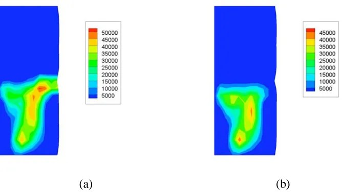
3.2.1. Dislocation-density Transmission

First a comparison is made between an aggregate without the DDGBI scheme and one with the DDGBI scheme. The dislocation-density evolutions of a 3 bicrystal are presented in Figs. 3.2-4 at a nominal strain of 20%. The immobile dislocation-density of the most active slip system 110

( )

1 11 is shown in Figs. 3.2a, 3.3a and 3.4a, and the immobile dislocation-density of a less active slip system,

[ ]

011

( )

1 11 is shown in Figs. 3.2b, 3.3b and 3.4b. The resolved shear stress is 0.85ref for the less active system. The transmission factor between these two slip systems is equal to 0.7, which indicates that there is a high possibility of dislocation-density transmission through the GB. The dislocation-densities on the active slip system (Fig. 3.2a) are much higher than the less active slip system (Fig. 3.2b). If there is no interaction mechanism between the GB and the dislocation densities, due to the reference stress being below the critical stress, the dislocation-densities of the less active slip system of the neighboring grain remain the same even though the possibility of dislocation transmission is high.

Predictive Microstructural Modeling of Grain-boundary Interactions and Their Effects on Overall Crystalline Behavior

ABSTRACT

Predictive Microstructural Modeling of Grain-boundary Interactions and Their

Effects on Overall Crystalline Behavior

Jibin Shi

DEDICATION

BIOGRAPHY

ACKNOWLEDGEMENTS

TABLE OF CONTENTS

LIST OF TABLES

LIST OF FIGURES

( )

( )

( )

( )

( )

( )

( )

( )

( )

( )

( )

CHAPTER 1

INTRODUCTION

1.1.

GB Effects and GB Misorientations

1.2.

Representation of GB Geometry and Coordinate Transformation

(

[

]

[

]

[

]

)

(

)

{

}

1.3.

Intergranular and Transgranular Cracks

1.4.

Grain Size Effect and Hall-Petch Relation

1.5.

Grain Boundary Sliding (GBS)

1.6.

Experimental and Computational Methods

( )

( )

CHAPTER 2

FORMULATIONS

2.1.

Dislocation-density Based Multiple-slip Crystal Plasticity Constitutive

Formulation

2.1.1.

(

)

(

)

(

)

(

)

(

)

(

)

2.1.2.

( )

2.1.3.

2.2.

Dislocation-density Grain Boundary Interaction (DDGBI) Scheme

(

)

(

)

(

)

2.3.