ABSTRACT
SMITH, MARK PRESTON: Predicting Fuel Models and Subsequent Fire Behavior from Vegetation Classification Maps. (Under the Direction of Dr. Hugh A. Devine)
The recent trends in wildland fires have created a level of motivation that requires
natural resource managers to predict fires through the use of computer based simulation
programs. Using vegetation maps delineated from large-scale aerial photography and fuel
loading values collected from fieldwork, I simulated how fire would react to changes in fuel
model assignments for Booker T. Washington National Monument (BOWA) and George
Washington Birthplace National Monument using FARSITE, a fire simulation program. The
environments for these fires were based on weather and fuel conditions found during the
summer and fall months for each area.
Sample points, stratified by vegetation formation, were selected. Then, field
measurements using Brown’s transect lines and Burgan and Rothermel ocular procedures
were used to calculate the amount of fuel loading in tons/acre for each sample point. These
values were then used to assign a fuel load to each vegetation formation class. Then each
vegetation polygon on the map was assigned one of the thirteen National Fire Fuel
Laboratory fuel models based on fuel load, vegetation type, and overall structure of the
surrounding area. The sampling results showed a one to one correspondence of fuel model to
vegetation formation.
The sensitivity of FARSITE was tested by changing fuel model layers within
FARSITE while holding all other variables constant (e.g., weather, moisture, etc.). Rate of
The results from the simulations showed that there was little sensitivity to changes in
the assignment of fuel models for forested vegetation for these sites. The rate of spread and
fire line intensity for grass fuel models showed sensitivity to changes in fuel model
PREDICTING FUEL MODELS AND SUBSEQUENT FIRE BEHAVIOR FROM VEGETATION CLASSIFICATION MAPS
by
MARK PRESTON SMITH
A thesis submitted to the Graduate Faculty of North Carolina State University
in partial fulfillment of the requirements for the Degree
of Master of Science
NATURAL RESOURCES,
SPATIAL INFORMATION SYSTEMS TECHNICAL OPTION
Raleigh
2003
APPROVED BY:
_______________________________ Dr. Hugh A. Devine, Chair of Advisory Committee
_______________________________ ______________________________
Dr. Stacy A. C. Nelson Dr. E. Carlyle Franklin
DEDICATION
This work is dedicated to my wife, Margaret, a true ray of sunshine in an otherwise
BIOGRAPHY
The author grew up in Fairfax, Virginia and has spent the past eight years living in
various places on the coast and in the piedmont of North Carolina. In 1995, he graduated
from Virginia Polytechnic Institute and State University with a bachelor’s degree in Forestry
and Wildlife Resources with a concentration in Outdoor Recreation. Immediately following
graduation, he started his career as a seasonal state park ranger on the coast of North Carolina
and later moved to Raleigh where he became a state park ranger for six years. His interest in
pursuing his knowledge of natural resources persuaded him to enroll at North Carolina State
University as a Master of Science student in Natural Resources, concentrating in spatial
information systems. He was awarded a research assistantship in the Center for Earth
Observation where he worked on vegetation mapping and moasicing of aerial photography
for several national parks.
His research interests are applying GIS and GPS to conserve and protect natural
ACKNOWLEDGEMENTS
I would like to express my sincere gratitude to the members of my thesis committee-
Dr. Hugh Devine, Dr. Stacy Nelson, and Dr. E. Carlyle Franklin. Likewise, I would like to
thank the graduate students and staff of the Center for Earth Observation: Brian Rosenfeld,
Mikey Neighbor, Andrew Bailey, Bill Slocumb, and Bill Millinor. I would especially like to
thank Frank Koch who was a constant savior when others were unsure of the answer.
Doug Raeburn and Dan Hurlbert from Shenandoah National Park were instrumental in
providing guidance and support with fire information and all around knowledge that never
seemed to present itself in books nor the internet. Karen Patterson from the Virginia Natural
Heritage program provided additional information with mapping the vegetation for George
Washington Birthplace National Monument and Booker T. Washington National Monument.
I would also like to thank my family who never seemed to stop believing in me- my
parents Jeff and Claudia Smith, Pat Henderson and Joe Phillips, and Frank and Barbara
Davide; my brothers Alex, Jason, Tim, Frank and their wives, and to all of my extended
TABLE OF CONTENTS
List of Tables ... viii
List of Figures... ix
1. Introduction...1
2.Literature Review ...3
2.1 Problems and risks of fires...3
2.1.1 Forest health...3
2.1.2 Development near forests ...4
2.2 Fire management techniques...4
2.2.1 Fire prevention...5
2.2.2 Wildland Urban Interface ...6
2.3 Review of fire modeling programs ...8
2.3.1 FARSITE ...8
2.3.2 BehavePlus...9
2.3.3 NEXUS ...10
2.3.4 FOFEM ...11
2.4 Review of fuel model and fuel loading guides ...12
2.4.1 Aids to determining fuel models for estimating fire behavior...12
2.4.2 National Fire Danger Rating System ...13
2.4.3 Photo guide for appraising surface fuels in east Texas...14
2.4.4 Inventorying downed woody material for Brown’s calculations...15
2.4.5 US Forest Service quick method...16
2.5 Similar fuel modeling and FARSITE research ...17
3. Study Areas...21
3.1 Booker T. Washington National Monument...21
3.2 George Washington Birthplace National Monument ...21
4. Objectives...23
5. Methodology ...24
5.2 Orthorectification...26
5.3 Creating the mosaic images ...27
5.4 Delineation of vegetation...28
5.5 Accuracy assessment ...30
5.6 Fuel data collection...32
5.7 Fuel data calculation ...34
5.8 Creation of FARSITE layers and simulating wildland fire conditions...34
6. Results ...40
6.1 Positional accuracy of the mosaiced images...40
6.2 Thematic accuracy for the vegetation layers ...42
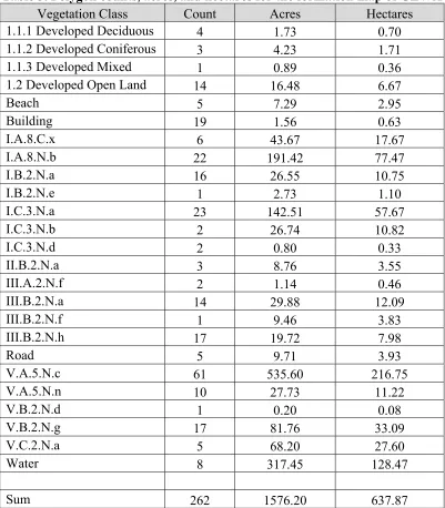
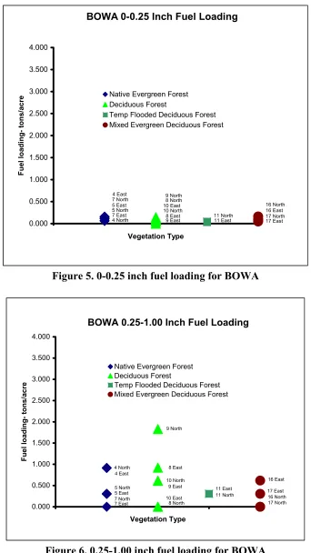
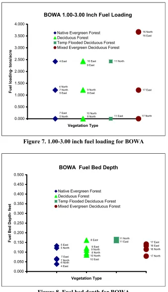
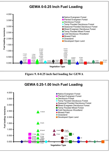
6.3 Fuel loading calculation and results...49
6.4 Standard sample size for estimating fuel load ...56
6.5 Fuel model maps ...58
6.6 FARSITE simulations...59
7. Discussion...76
7.1 Creation of orthoimage mosaics ...76
7.2 Vegetation map accuracy...76
7.3 Fuel loading calculations ...77
7.4 FARSITE simulation ...78
8. Conclusion and Recommendations ...80
References...83
Appendices...88
Appendix A. Fall mosaic of Booker T. Washington National Monument ...88
Appendix B. Spring mosaic of Booker T. Washington National Monument...89
Appendix C. Fall mosaic of George Washington Birthplace National Monument ...90
Appendix D. Spring mosaic of George Washington Birthplace National Monument ...91
Appendix F. Fuel model maps for Booker T. Washington Monument ...94 Appendix G. Fuel model maps for George Washington Birthplace National
Monument ...100 Appendix H. Error matrix of the vegetation map thematic accuracy assessment
of Booker T. Washington National Monument ...106 Appendix I. Error Matrix of the vegetation map thematic accuracy assessment of George Washington Birthplace National Monument ...107
Appendix J. Brown’s transect datasheet ...118 Appendix K. Burgan and Rothermel datasheets ...109 Appendix L. Fuel loading values for sample plots at Booker T. Washington National Monument ...111
Appendix M. Minimum sample size calculations for Booker T. Washington National Monument ...114
Appendix N. Fuel loading values for sample plots at George Washington
Birthplace National Monument...116 Appendix O. Minimum sample size calculations for George Washington
Birthplace National Monument...126 Appendix P. Combined minimum sample size calculations ...131
LIST OF TABLES
Table 1. Physiognomic-floristic hierarchy of the NVCS...30
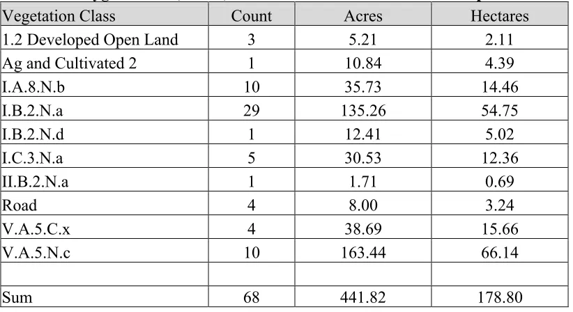
Table 2. Polygon counts, acres, and hectares for the formation map of BOWA...42
Table 3. Polygon counts, acres, and hectares for the formation map of GEWA ...46
Table 4. Standard sample sizes for BOWA ...57
Table 5. Standard sample sizes for GEWA ...57
Table 6. Standard sample sizes for combined vegetation ...58
Table 7. BOWA simulation results using assigned fuel models...60
Table 8. BOWA simulation results using adjusted fuel models ...60
Table 9. BOWA simulation results holding grass formation fuel models constant...61
Table 10. GEWA simulation results using assigned vegetation ...62
Table 11. GEWA simulation results using adjusted vegetation ...62
LIST OF FIGURES
Figure 1. Map of Booker T. Washington National Monument...22
Figure 2. Map of George Washington Birthplace National Monument ...22
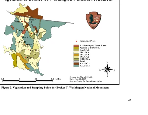
Figure 3. Vegetation and sampling points for Booker T. Washington National Monument ...43
Figure 4. Vegetation and sampling points for Booker T. Washington National Monument ...47
Figure 5. 0-0.25 inch fuel loading for BOWA...51
Figure 6. 0.25-1.00 inch fuel loading for BOWA...51
Figure 7. 1.00-3.00 inch fuel loading for BOWA...52
Figure 8. Fuel bed depth for BOWA ...52
Figure 9. 0-0.25 inch fuel loading for GEWA ...54
Figure 10. 0.25-1.00 inch fuel loading for GEWA ...54
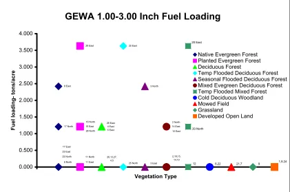
Figure 11. 1.00-3.00 inch fuel loading for GEWA ...55
Figure 12. Fuel bed depth for GEWA...55
Figure 13. Summer assigned fuel models rate of spread for BOWA ...64
Figure 14. Summer assigned fuel models fire line intensity for BOWA...64
Figure 15. Fall assigned fuel models rate of spread for BOWA...65
Figure 16. Fall assigned fuels model fire line intensity forBOWA ...65
Figure 17. Summer adjusted fuel models rate of spread for BOWA...66
Figure 18. Summer adjusted fuel models fire line intensity for BOWA ...66
Figure 19. Fall adjusted fuel models rate of spread for BOWA ...67
Figure 21. Summer assigned grass fuel models rate of spread for BOWA ...68
Figure 22. Summer assigned grass fuel models fire line for BOWA ...68
Figure 23. Fall assigned grass fuel models rate of spread for BOWA ...69
Figure 24. Fall assigned grass fuel models fire line for BOWA...69
Figure 25. Summer assigned fuel models rate of spread for GEWA...70
Figure 26. Summer assigned fuel models fire line intensity for GEWA ...70
Figure 27. Fall assigned fuel models rate of spread for GEWA...71
Figure 28. Fall assigned fuels model fire line intensity GEWA ...71
Figure 29. Summer adjusted fuel models rate of spread for GEWA ...72
Figure 30. Summer adjusted fuel models fire line intensity for GEWA ...72
Figure 31. Fall adjusted fuel models rate of spread for GEWA ...73
Figure 32. Fall adjusted fuel models fire line intensity for GEWA...73
Figure 33. Summer assigned grass fuel models rate of spread for GEWA ...74
Figure 34. Summer assigned grass fuel models fire line for GEWA...74
Figure 35. Fall assigned grass fuel models rate of spread for GEWA...75
1. INTRODUCTION
According to the National Interagency Fire Center website
(http://www.nifc.gov/index.html), approximately seven million acres of forests burned across
the country during the 2002 fire season. The high numbers of acres lost to fire has promoted
the development of computer simulations to predict and consequently manage forest fires.
The creation of fuel models is integral to these simulations. Fuel models are a set of
numerical values that describe the amount of fuel present within a natural setting. Fuel is
defined as any substance that can burn such as sticks, grass, and leaf litter. Through the use
of fuel models, the U.S. Forest Service created several approaches to estimate how fires will
react under certain conditions. The National Forest Fire Laboratory (NFFL) fuel models are
comprised of thirteen fuel models that estimate fuel loading from four separate fuel types
(grasses, brush, timber, and slash). These types are further broken down into measures of
fuel loading for fine and course downed woody debris, fuel bed depth, and moisture of
extinction. These measures for the fuel models are collected in the field using transect lines
developed by James K. Brown (1974).
The NFFL fuel models are dependent upon vegetation found within designated areas.
By correlating the amount of fuel found within each vegetation class, fuel models can be
assigned to these classes. Currently, the amount of sampling required to estimate fuel
loading using standard sampling procedures is prohibitive (e.g. 2800 sample sites at George
Washington Birthplace National Monument). Predicting fuel models from an existing
national vegetation mapping program would dramatically reduce the cost of fuel load
formation level vegetation maps for Booker T. Washington National Monument (BOWA)
and George Washington Birthplace National Monument (GEWA) for summer and fall
conditions. A secondary goal was to evaluate the sensitivity of FARSITE (Finney 1998)
simulation results relative to the variations in fuel model predications for the above two
parks. To accomplish this goal, I varied the fuel model inputs to FARSITE and observed the
2.LITERATURE REVIEW
This literature review describes the problems associated with fire and management
techniques currently being used in the natural resources field. Several fire simulators and
fuel model guides will be compared and evaluated to show why FARSITE and Brown’s
transect lines were utilized in this research project. Finally, projects with similar fuel loading
and FARSITE research will be compared.
2.1 Problems and risks of fire
The Forest Service has stated that nearly 73 million acres of national forests (61
million in the West and 12 million in the East) are at high to moderate risk of catastrophic
fire (Alvarez 2003). This risk is due to a lack of fire management techniques that reduce the
amount of fuel loading. According to the National Interagency Fire Center, 1.6 billion
dollars was spent in 2002 to suppress and protect forests as well as areas adjacent to these
lands. The damage from fire is detrimental to forests and negatively impacts the
development of urbanized areas that are encroaching on natural areas.
2.1.1 Forest Health
The lack of fire within national forests and public lands has increased the chance for
fire to occur. The suppression of fire in these areas by natural resources managers has
contributed to fuel buildup, prevented tree stocking, and increased the population of endemic
natural areas. Large, intense wildfires have proven difficult to control and have resulted in
catastrophic damage to property and resources, and the tragic loss of lives (SAF 2002).
While these fires can damage ecological conditions, areas will eventually regenerate to their
natural characteristics.
2.1.2 Development near forests
A surge in development near forested and natural areas has increased the risk of
damage to these areas by fire. The area where structures and other human developments
meet or blend together with undeveloped wildland or vegetative fuels is known as the
“wildland urban face” (Federal Register 2001). According the FIREWISE, a program
developed to educate the public about the hazards of living in the wildland urban interface,
88,458 fires occurred during the 2002 fire season (FIREWISE 2003). Despite a cost to
federal agencies of $1.6 billion dollars to suppress, a total of 815 structures were burned.
These totals highlight the fact that as development continues to intermix with wildland
settings, fire will destroy more houses and developed areas.
2.2 Fire management techniques
The management of fire involves numerous methods to reduce fuel loading and
prevent fire. An important feature of these techniques is the use of a geographic information
system (GIS). GIS programs allow managers to administer fire on a spatial scale in a
of wildland fire and the actual plan to its suppression. GIS also allows the interactive display
of historical fire information and the rapid infusion of new fuel data to these map documents.
2.2.1 Fire prevention
The suppression of fire in many landscapes has increased the amount of available fuel
to be burned in wildland fires. The Mineral King Valley, located in Sequoia National Park,
has suppressed fires for several seasons and as a result, fuel loads have increased (Menning et
al. 1998). This has affected the regeneration of trees and increased the risk to insect attacks
and disease. Several researchers from the University of California at Berkeley are using
prescribed burning to reduce the amount of fuel loading and allow regeneration of many
suppressed tree species (Menning et al. 1998). Researchers are also measuring the
effectiveness of prescribed burning by establishing field plots randomly located throughout
the valley. Within each plot, field crews record tree characteristics, fuel loading conditions,
brush and plant conditions, slope and aspect, and light penetration. Aerial photographs also
provide an additional source of information for the field crews to assess forest health and
results of the prescribed burn. The results from this study are ongoing and are currently
being published.
Keifer et al. (2000) looked at twenty-seven plots located in the Sequoia and Kings
Canyon National Parks in southern California. The plots were located within areas burned
between 1982 and 1997. Monitoring data, fuel load, and tree density were recorded for
pre-burn, immediately post-pre-burn, and 1, 2, 5, and 10 year post burn conditions for each plot. The
burning was successful in reducing fuel loading and restoring giant sequoia-mixed conifer
forest.
van Wagtendonk et al. (2002) created a fire management regime that included
prescribed burning for Yosemite National Park. The plan incorporated the use of a
geographical information system (GIS) along with previous experience from Keifer et al.
(2000) to monitor prescribed burning in the park. It was found that an effective fire
management plan requires spatial and non-spatial data. This information has allowed the
managers to restore the natural fire regime in many areas of the park.
2.2.2 Wildland Urban Interface
People are building homes and communities closer to wooded areas every day. These
communities are also developing near federally owned lands such as national parks and
forests. The close proximity of development near housed has increased the chance of loss
due to fire from surrounding areas. A program called FIREWISE COMMUNITIES was
developed by the National Wildland/Urban Interface Fire Program to aid communities in
effectively protecting them from damage caused by wildland fires (National Wildland Urban
Interface Fire Program 2001). The program reviews the problems communities may face by
being close to the wildland urban interface and assigns a hazard severity rating based upon
history of the development, vegetation types, fuel loading, access routes, land use
information, and fire protection capabilities. A GIS plays an integral part in mapping these
communities and its surrounding areas to provide residents with an idea of where high-risk
communities to prevent damage from wildland fires. It also allows natural resource
managers to identify high-risk communities and target them first to prevent further fires from
spreading and damaging more homes as well as forests.
Mattsson and Thoren (2002) developed a wildland/urban interface model using GIS for
the town of Pocatello, Idaho based on vegetation characteristics and fire suppression access.
The input layers into the model were slope, aspect, and fuel loading. The slope and aspect
layers were created from a USGS digital elevation model (DEM) and the loading assessment
was performed using a supervised classification from a Landsat 7 Enhanced Thematic
Mapper image. The input layer results were assigned a weighted value in order to reach an
overall hazard rating value. The program provides communities as well as natural resource
managers with information on areas having a high risk of damage from wildland fires.
Radke (1995) developed a spatial decision support system (SDSS) so planners and
decision makers could better manage and formulate policy to help reduce the risk of future
fires in the East Bay Hills of California. The system combines two models: one to assess the
wildland fire hazard and the second to assess the urban/residential fire hazard within a GIS to
map risk areas for the region and neighborhood. The wildland fire hazard was rated based on
weather, topography, and fuel type and the urban/residential fire hazard rating was based on
structural and vegetation fuels. The wildland vegetation layer was delineated using aerial
photographs and assigned a fuel model correlating with the Anderson (1982) fuel model
guide. The fuel models were then simulated in BEHAVE (Andrews 1986) to obtain flame
length, rate of spread, heat released, and crowning potential. The urban/residential fire
were then combined to produce an overall rating for the East Bay Hills area to provide
decision makers with the information necessary to prevent future wildland fires.
2.3 Review of Fire Modeling Programs
The following section will provide a brief description about existing programs that simulate fire as well as allow the user to create custom fuel models. There are several
different types of programs under development to predict fire and its characteristics. This
section clarifies the differences between the various programs and justifies the use of
FARSITE in this project.
2.3.1 FARSITE
Dr. Mark Finney from the U.S. Forest Service Rocky Mountain Research station
created Fire Area Simulator (FARSITE) to simulate growth and fire behavior as it spreads
through different fuel types and terrain patterns. The program is based on Huygens’
principle that states the spread direction and rate of the fire are based on an elliptical
transformation (Finney 1998). The transformation calculates ellipse shape and direction
based on wind and slope characteristics for an area. It also calculates ellipse size based on
fire spread rate and length of time step for the simulation.
FARSITE requires spatial and non-spatial layers created by the user. A Geographic
Information System (GIS) is used to create the spatial layers for each simulation. Three
required spatial layers are derived from elevation grids. These are elevation, slope, and
represents the percent of an area covered by vegetation canopy while the fuel model layer is
derived from the National Fire Fuel Laboratory fuel models (Anderson 1982). The
remaining FARSITE inputs are non-spatial and are created from existing weather conditions
for the area where the fire will be simulated.
The outputs from FARSITE can be created either as a GRASS ASCII or GRID ASCII
format. The user has the option of choosing from the following output grids: time of arrival,
fireline intensity, flame length, rate of spread, heat / area, reaction intensity, crown fire
activity, spread direction. All of these grids can then be analyzed in a GIS to predict and
manage for current wildfire or plan for future fires.
2.3.2 BehavePlus
BehavePlus was created by Patricia L. Andrews, currently working with the USDA Forest Service, Rocky Mountain Research Station, and Collin Bevins, Systems for
Environmental Management. This program runs fire simulation models for BehavePlus
inputs of surface fire spread, intensity, flame length, area and perimeter of a point source fire,
spotting distance, probability of ignition, scorch height, and tree mortality (Andrews and
Bevins 1998). The user enters information on “worksheets” that are provided within the
program. These “worksheets” are then manipulated in the program to produce several
outputs such as rate of spread, heat per unit area, fireline intensity, flame length, etc. These
outputs can be displayed in either graphical format (non-map) or tabular format.
There are several differences between FARSITE and BehavePlus. BehavePlus makes
load, weather, and topography. This is unlike FARSITE which predicts fire growth across a
given landscape for variable fuel loads, weather, and topography. BehavePlus inputs can be
determined easily in the field while FARSITE inputs require extensive GIS support and
theme development (Carlton 2001). FARSITE allows the user to define the point of ignition
in the landscape while the user has to change the worksheet settings in BehavePlus to
simulate a wildfire at a different position. Finally, BehavePlus also allows the user to create
custom fuel models based on measurements collected in the field while FARSITE only
allows the user to input custom fuel models into the simulation.
2.3.3 NEXUS
Joe Scott, Systems for Environmental Management, and Elizabeth Reinhardt, Missoula
Fire Sciences Laboratory, developed NEXUS in 1999 as a spreadsheet program to couple
Rothermel’s (1972) surface fire and (1991) crown fire models to simulate the full range of
behavior possible in a forest stand (Scott 1999). Among its capabilities, NEXUS is able to
predict surface fires, passive crown fires, and active crown fires. Prediction of crown fires is
particularly important since they greatly affect the intensity and rate of spread of a fire.
The user enters information for surface and crown fire on a spreadsheet provided with
the program. The information of surface fires consists of fuel models (standard or custom),
live and dead surface fuel moistures, slope, 20-foot wind speed, wind reduction factor, and
wind direction. For crown fires, the user enters crown base height and crown bulk density.
The output from NEXUS is similar to BehavePlus but it includes the type of fire
within the Excel spreadsheet. NEXUS also can create charts and graphs of selected fire
characteristics such as spread rate and flame length, crown fire hazard assessment, and fire
characteristics (Scott 1999).
Major differences between NEXUS and FARSITE include; NEXUS is only able to
compute fire behavior information for up to six spatial areas while FARSITE is unlimited in
its spatial extent. Additionally, NEXUS information is only in tabular or graphical form
while FARSITE creates grids that can be displayed in a GIS. FARSITE is more applicable
than NEXUS for this project since both study areas have significantly more vegetation areas
as well the map output will an provide more detailed information about the fire.
2.3.4 FOFEM
Bob Keane, Elizabeth Reinhardt, Jim Brown, and Larry Gangi with the Intermountain
Fire Sciences Laboratory developed First Order Fire Effects Model (FOFEM) to meet the
needs of resource managers, planners, and analysts in predicting and planning for fire effects
(Reinhardt, Keane, and Brown 1998). FOFEM version 5.0, created in 2002, provides users
with fire effects information about tree mortality, fuel consumption, smoke, and soil heating.
FOFEM provides forest cover types for four geographical regions within the United States:
the Pacific West, Interior West, Northeast, and Southeast.
The program uses a Microsoft Windows Operating System based graphical user
interface (GUI) to allow for easy data entry into the program. Inputs are based on the
Anderson fuel models (Anderson 1982): litter surface fuels, vegetation cover type, litter,
load, stand height, crown base height, dead and live fuel moisture, and soil moisture
(FOFEM 2003). The program provides defaults for the above values and the user is able to
change these values.
The outputs from FOFEM are fuel consumption, smoke production, emissions, fire
intensity, tree mortality, and soil heating. This information can be presented in table and
graphical format to the user.
There are several differences between FOFEM and FARSITE. The major differences
are similar to BehavePlus and NEXUS in that fire simulation is limited to a few stands and
the output results can only be displayed as graphs or tables.
2.4 Review of Fuel Model and Fuel Loading Guides
The following section provides a brief description of existing fuel models and fuel
loading guides that provide natural resource managers the means to predict fire behavior.
This section clarifies the differences between various guides and justifies the use of the
Anderson (1982) fuel model guide and fuel loading calculations developed by Brown.
2.4.1 Aids to Determining Fuel Models for Estimating Fire Behavior
Hal E. Anderson created a guide to assist natural resource managers in predicting fire
behavior through the use of photographic illustrations. This guide was developed from
thirteen fuel models calculated by Rothermel (1972) and Albini (1976) to estimate fire
behavior predictions. The fuel models are broken down into four different fuel groups:
essentially related to the fuel load and its distribution among the fuel particle size classes
(Anderson 1982). For each of the fuel groups, a series of photographs are provided that
describe a “potential” scene of what this model may look like in a natural setting. A brief
description is also provided to define “potential” field characteristics present in a particular
fuel model. Fuel loading values, fuel bed depth, rate of spread, flame length, and moisture of
extinction for dead fuels are also provided for each fuel model. Finally, a correlation value
chart to the National Fire Danger Rating System is provided for each fuel model within the
guide. This guide is widely accepted by fire managers since it provides pictures of what a
typical area would look like given the specific fuel model. It is also prevalent in a majority
of fire simulators found within the natural resources/fire management field.
2.4.2 National Fire Danger Rating System
The National Fire Danger Rating System (NFDRS) was originally developed in 1972
to produce an analytical system based on the physics of moisture exchange, heat transfer, and
other aspects associated with fire. The system produces three indexes of occurrence,
burning, and fire load based upon four fire components consisting of risk, ignition, spread,
and energy release (Deeming 1972). The indexes provide a day-to-day guide for fire
managers to assess the potential for fire in a wildland setting. The 1972 NFDRS produced
nine fuel models based on the amount of fuel loading for each wildland area. This system
was revised in 1978 to address several shortfalls in the original system. The 1978 version of
NFDRS included 11 new fuel models (which increased the total to 20 models overall) to
and identify a better way to assess live fuel conditions (Deeming et al. 1977). The 1978
NFDRS was updated again in 1988 to improve the capability to respond to drought in humid
environments, adjust fuel models to better predict fire danger in humid climates, correct for
the overrating of fire danger in the autumn and after rainfall, and reflect the greening and
curing of live fuels (Burgan 1988).
The twenty fuel models within the 1988 NFDRS are grouped into six general classes
defined by their predominant surface fuel: lichens and mosses; marsh grasses and reeds;
grasses and forbs; brush, shrubs and tree reproduction; trees; and slash (Schlobohm and Brain
2001). These surface fuel sources are further broken down into sub-classes that comprise the
twenty fuel models. There is a section within the NFDRS that correlates to the thirteen fuel
models that are presented in the guide produced by Anderson (1982).
The NFDRS is different from the Anderson fuel model guide in that it presents a fire
hazard rating system that natural resource managers can follow. The Anderson fuel model
guide is more applicable since this project only deals with simulating fire instead of
estimating fire danger rating.
2.4.3 Photo Guide for Appraising Surface Fuels in East Texas
Dr. Hershel C. Reeves created a photo guide in 1988 to depict different levels of fuels
ranging from open grassy conditions to dense pine plantations (Reeves 1988). A total of nine
different photo series taken in east Texas were used to assist natural resource managers in
selecting fuel models including, grass, clear cut, seed tree, loblolly/shortleaf pine, slash pine,
with a data sheet describing the down and dead woody fuel loadings, litter and herbaceous
loading, fire potential rating, and other fuel data. Dr. Reeves included a NFDRS fuel model
and a stylized fuel model for each plot within the guide. The stylized fuel model directly
correlates with Anderson fuel model guide (Anderson 1982).
This guide is similar to the one produced by Anderson (1982) but it provides different
plot pictures and fuel loading values. It also breaks down potential fuel sources into nine
different photo series. This photo series along with the one created by Anderson (1982)
provides natural resource managers with greater capability to assign fuel models to
vegetation found in the field.
2.4.4 Inventorying Downed Woody Material for Brown’s Calculations
A handbook was developed by James K. Brown that defined how to inventory downed woody debris material using a vertical sampling plane and entering this information into a
provided formulas to estimate the amount of fuel loading in tons per acre (Brown 1974). The
handbook provides users with guidelines to locate sampling plots, tally rules, necessary field
equipment, and other information to be used in calculating the amount of fuel loading. The
data collected at each sampling plot is then entered into either one of two formulas known as
Brown’s calculations. The first formula calculates the amount of fuel loading for downed
woody debris that is 0 – 3 inches in diameter. Components of the formula include number of
intersects along the sampling plane, squared average diameter, specific gravity, horizontal
angle correction factor, and a slope correction value. The second formula calculates the
of the formula are the same except that the diameters of the downed woody debris are
squared and the debris is classified as rotten or sound. The result of both formulas provides
an amount of fuel loading for each size class in tons per acre.
Brown’s handbook is used to estimate the amount of fuel loading in wildland settings.
The National Park Service uses this method and has created their own handbook for field
staff to use (USDI NPS 2001). This handbook includes field collection protocol procedures
along with protocols to monitor vegetation, pre and post-burn fire plots, and data analysis.
The data that was collected for my research will be used by the National Park Service so all
the defined protocols in this book were used in the field.
2.4.5 US Forest Service Quick Method
The quick method was developed by Cary Rouse and Donna Paananen from the US
Forest Service North Central Forest Experiment Station to allow fire managers to make rapid
and accurate estimates of fuel loading in the field (Rouse and Paananen 1988). A condensed
formula from Brown’s calculation and measurements from a planar intersect line (Brown
1974) are used to calculate the amount of fuel loading for a specific area. Planar intersect
size classes of downed woody debris are 0 - ¼ inches, ¼ - 1 inch, and 1 -3 inches. The user
then applies one of several provided composite factors for each of the three size classes to the
formula. The final result is an estimate for the amount of fuel loading in tons per acre for
each size class.
A problem with the condensed formula is that it uses more Northeastern fuel types so
the amount of fuel loading was not well documented and very few agencies have used this
method to estimate fuel loading.
2.5 Similar fuel modeling and FARSITE research
Several methods have been used to estimate fuel models based on remotely sensed
images. Scott et al. (2002) used aerial photographs to estimate fuel loading for the Sanger de
Cristo (Santa Fe watershed) and Jemez mountains (Los Alamos National Laboratory) of New
Mexico. The purpose of their research was to create fuel load prediction equations based on
pine composition, pine basal area, and crown closure information acquired from aerial
photos. Large-scale aerial photographs (1:15840) were used to delineate different vegetation
types within the two areas. A total of 60 sample sites were used for the Santa Fe Watershed
(SFWS) and 56 sample sites were used for the Los Alamos National Laboratory (LANL).
Field data collected at the two study areas included fuel loading values based on Brown’s
(1974) transect lines, tree species, canopy density and height. A fuel model was assigned to
each of the plots based on the field data collected and also on the photo guide developed by
Reeves (1988). Scoot et al. created an equation that produced similar fuel loading values
from aerial photographs compared to field sampling values for the SFWS. Unfortunately,
they were not able to predict these values for the LANL. Similar research conducted by
Oswald et al. (1999) found that fuel models could be successfully estimated from aerial
photography. That study did assign fuel models to vegetation found within the two study
areas but it did not use any fire spread models to estimate how the study areas would react to
Keane et al. (2000) created fuels and vegetation spatial layers for FARSITE for the
Gila National Forest located in New Mexico. This included: elevation, slope, aspect, fire
behavior fuel models (FBFM), canopy cover, average stand height, average crown base, and
crown bulk density. The GIS layers were created from field data, satellite imagery (using
Landsat TM), and local knowledge. Areas with unique vegetation types were delineated
using textural classification methods. A supervised classification was then used to assign
vegetation categories. A total of 1,000 sampling plots, each 405 m2 in size, were used to
collect fuel loadings, tree size distributions, plant species compositions, ecological attributes,
and stand characteristics. The fuel loading was measured using Brown’s (1974) method at
890 of points located in the National Forest. Sixty-foot transect lines facing east were used
to estimate the amount of fuel loading while my research utilized 50 foot lines. Also, fuel
bed depth was measured at the 35 and 60-foot marks instead of every five feet and at least 3
transect lines were used to measure intersects instead of two. The fuel loading along with
field measurements was used to assign one of the thirteen fuel models (Anderson 1982). The
remaining input layers were created from field measurements and were incorporated into the
remaining layers. This study did not create a simulation for the Gila National Forest but it
did create similar layers that were used for FARSITE.
Troy et al. (1998) created a FARSITE simulation for Strawberry Canyon in the East
Bay Hills area of California north of Berkeley and Oakland. The objective of their study was
to create a defensible fuel profile zone (DFPZ) along the ridge between Claremont and
Strawberry Canyon to protect structures along a panoramic drive. A cost/benefit analysis
input layers for this project were created using a digital elevation model (DEM), black and
white aerial photography with a 2-foot resolution, and local information. The vegetation and
canopy layer were created using a supervised classification to define different vegetation
found within the study area. The fuel models were assigned using the classification and local
knowledge of the vegetation. Several manipulations were tested to determine the most
beneficial management plan for the study area including reducing the fuel model by 2,
starting the fire at several ignition points, and varying the area of the fire to be burned. This
study provided some insight into how different simulations from FARSITE affect the cost of
the proposed management plan.
Etlinger et al. (1999) also created a FARSITE simulation for Claremont Canyon, in the
same region as Troy et al. The purpose of their simulation was to prepare a management
strategy using FARSITE to reduce fire potential and increase feasible habitat for the federally
threatened Alameda snake. The input layers into FARSITE were created from an existing
vegetation layer and fieldwork. The vegetation coverage was provided by the East Bay
Vegetation Consortium but was clipped down to the study area. The fuel layer was created
from the vegetation layer by assigning a fuel model to each vegetation type. The crown base
height and crown height layers were collected from fieldwork. The crown bulk density was
enabled in FARSITE by linking crown density and canopy cover. The canopy cover layer
was created by classifying 1:24000 black and white aerial photographs into four canopy
classes instead of recording this measurement from fieldwork. A total of four different
treatments were simulated in FARSITE: no action (treatment 0), reduction of fuel load of
to 1 (treatment 2), and reduction of oak-bay woodland from fuel model 4 to 8 (treatment 3).
The results from the simulation found that treatment 1 and 3 burned fewer acres than
treatment 0 and treatment 2 increased the total acreage burned.
The previous studies did not test the correlation of fuel load and subsequent fuel model
with field data. In addition, they did not examine the sensitivity of FARSITE results to
3. STUDY AREAS
3.1 Booker T. Washington National Monument
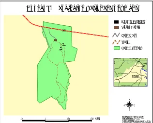
Booker T. Washington National Monument (BOWA), located 22 miles southeast of
Roanoke in Hardy, Virginia, is the birthplace of Booker T. Washington (Figure 1). The 224
acres surrounding the Burroughs farm where Booker T. Washington was born was dedicated
as a national monument in 1957 (NPS, 1995). The vegetation map of Booker T. Washington
created for my thesis research included areas that bordered the park. From this map,
approximately 214 acres were forested, 202 acres were grass fields, and 11 acres were
agricultural fields.
3.2 George Washington Birthplace National Monument
George Washington Birthplace National Monument (GEWA) in Virginia is the
ancestral home of George Washington (Figure 2). The 394-acre plantation including several
historical structures was dedicated as a National Monument in 1932 (NPS, 2001). The
vegetation map of George Washington created for my thesis research included areas that
bordered the park. From this map, 436 acres were forested, 9 acres were woodland, 61 acres
ø
÷
1 2 20.3 0 0.3 0.6 Miles
Booker T. Washington National Monument
Park Boundary Park Roads
Trails
Historic Buildings Visitor Center
Created by: Mark P. Smith Date: August 13, 2003 Data Source: National Park Service
r
.
-,8 1 .
-,9 5
Virginia
N E W
S
Figure 1. Map of Booker T. Washington National Monument
ø
÷
2 04Potomac River
Pope s Cree
k
0.5 0 0.5 1 Miles
N E W
S
George Washington Birthplace National Monument
Park Boundary Trails Park Roads Visitor Center Historic Buildings
Created by: Mark P. Smith Date: August 13, 2003 Data Source: National Park Service
r
.
-,8 1 .
-,9 5
Virginia
4. PROJECT OBJECTIVES
The following are my research objectives for this project:
• Develop an automated method to predict both summer and fall condition fuel models
from formation level vegetation maps for Booker T. Washington National Monument
and George Washington Birthplace National Monument.
• Evaluate the sensitivity of FARSITE simulation results relative to the variations in
5. METHODOLOGY
The process for developing an automated method to predict both summer and fall condition fuel models began with preparing photo mosaic images of both study areas. From
these images, vegetation maps were created by delineating vegetation based upon the
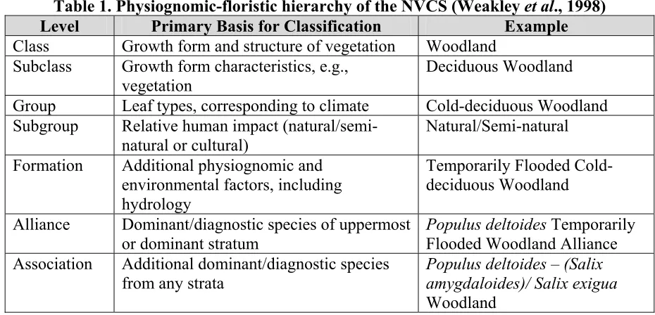
National Vegetation Classification system (Weakely et al. 1988) to the formation level. The
vegetation maps were then used to locate sample points stratified by formation. Brown’s
transect lines and Burgan and Rothermel ocular measurements were used to estimate the
amount of downed woody debris found at the sample sites. The amount of downed woody
debris provided an estimate for the amount of fuel loading found for each formation sampled.
Based upon the amount of fuel loading measured in the field, fuel models were assigned to
the formation classes for each study area.
In addition, the sensitivity of FARSITE to the variations in the fuel model assignment
was tested. The following section describes how each of the steps was completed to achieve
the objectives for this project.
5.1 Data Preparation
The creation of an aerial photo mosaic for each study area started with acquiring the
aerial photos. Kucera International, Inc. acquired the color-infrared (CIR) aerial photographs
for both study areas at a target scale of 1:6000 in leaf-on and leaf-off conditions. For
GEWA, twenty-four aerial photographs with leaf-on conditions were captured on October
20, 2001 and twenty-three aerial photographs with leaf-off conditions were captured on
October 22, 2001 and ten aerial photographs with leaf-off conditions were captured on
February 19, 2002 for BOWA. Kucera International, Inc. also provided airborne GPS
measurements and inertial measurement units (IMU) for each of the four photo missions
mentioned above in a *.dat (ASCII text) file format.
The CIR aerial photographs for both study areas were scanned using an Epson
Expression 836 XL or an Epson Expression 1640 XL desktop scanner. Each image was
scanned with 24-bit color, no filters, and at a 600 dot-per-inch (dpi) scanning resolution and
then imported into Adobe Photoshop 6.0. Each scanned image was cropped to reduce the
amount of black edges while still preserving the fiducials. The images were then saved as a
Tagged-Image File Format (TIFF). The aerial photographs for each study area were darker
in comparison to images used in similar projects. To correct for this, the TIFF images were
adjusted in Adobe Photoshop 6.0 using Auto Levels command. This command moves the
levels in the image to automatically set highlights and shadows. It defines the lightest and
darkest pixels on the image and then redistributes intermediate pixel values proportionately
(Adobe 2001). The TIFF images were then converted to *.img files in ERDAS Imagine 8.5
(ERDAS Imagine’s native file format).
Four USGS 7.5-minute digital elevation models (DEMs), corresponding to the Hardy,
Goodview, and Moneta, Virginia quadrangles were obtained for BOWA. Three DEMs,
corresponding to the Colonial Beach South, Stratford Hall, and Rollins Fork, Virginia
quadrangles were obtained for GEWA. The DEMs were acquired from the Radford
University GIS website, USGS seamless data website, and from the parks. These DEMs
GEWA were brought into ESRI ArcInfo where a focal mean was run to remove the seam
between the three DEMs. Richard Easterbrook, GIS Specialist for Petersburg National
Battlefield, provided the park boundary coverage for BOWA. Rijk Morawe, Natural and
Cultural Resources Management Chief for GEWA, provided the GEWA boundary using
existing survey maps for the area. The DEMS were resampled in ESRI ArcInfo GRID using
a cubic convolution algorithm (i.e. from 30-meters resolution to 10-meters) to match the
ground resolution of the scanned aerial photographs. The DEMS along with the airborne
GPS and IMU have projection settings of UTM NAD 83 18 North meters for GEWA and
UTM NAD 83 17 North meters for BOWA.
5.2 Orthorectification
The process of orthorectification was completed in ERDAS Imagine’s OrthoBase. This
program uses “block files” to store platform characteristics and interior and exterior
orientation. In the block files, the projection was set according to the *.dat file. A camera
calibration report containing focal length and fiducial information provided by Kucera
International, Inc. was used in the block file. The *.dat file was brought into the block file
for ground control. The next step was to attach all the scanned aerial photographs in *.img
format to the block file. The interior orientation for each block file was established using the
Frame Editor in OrthoBase. The correct fiducial orientation for each image was selected
from the four possible choices based upon flight direction of the platform. Fiducials were
then marked on each image using the Frame Editor until the root mean squared error (RMSE)
exterior settings from “initial” to “fixed” established the exterior orientation for each block
file. Once all of the parameters were set for each block, each image was resampled using
bilinear interpolation to create orthophotos using a batch process in OrthoBase.
5.3 Creating the Mosaic Images
The orthorectified images from the four flight missions were mosaiced into one image
for each of the study areas. The spring aerial photography from BOWA and the spring and
fall aerial photography for GEWA were mosaiced in ERDAS Imagine 8.5 using the Mosaic
Images tool. An area of interest (AOI) layer was selected on each image using the AOI Tool.
The center area was chosen on each image since distortion was at a minimum and there was
no sidelap or endlap from adjoining photographs (Avery and Berlin 1992). Each orthophoto
and its AOI were brought into the mosaic tool. The “no cutline” and “feather” options were
chosen under the mosaic options. The no cutline option was chosen since the AOI for each
image acted as the cutline. The feather option was chosen because it has been shown to be
an effective option when moasicing aerial photographs (Millinor 2000). Finally, the nearest
neighbor interpolation method was used to create the mosaic. The resulting output file size
for each mosaic was large and was subsequently compressed using the MrSID Geospatial
Encoder 1.4 (Multi-resolution Seamless Image Database) compression program from
LizardTech, Inc. The ratio of compression for each image was 20:1.
The fall mosaic for BOWA was created with ER Mapper 6.2, a program developed by
Earth Resource Mapping Ltd. This software mosaics images in a similar fashion to ERDAS
for BOWA were converted to LAN files in ERDAS Imagine 8.5 and then brought into ER
Mapper. They were then converted to *.ers files, the native file format for the program,
using an ESG_Import_LAN_Batch.erb batch script provided by ER Mapper. The *.ers files
where then mosaiced to create one seamless image using the mosaic tool within ER Mapper
6.2. It was then color balanced using no black and white edges. An algorithm with these
settings was saved for each of the images so they could be opened again without having to
reload all the images and reset the preferences. The final mosaic was saved as a *.bil file in
ER Mapper and converted in ERDAS Imagine to an *.img file using a generic binary format.
The final mosaic was compressed using the MrSID compression tool at a rate of 20:1.
5.4 Delineation of Vegetation
The unique vegetation types found within each study area was delineated in ERDAS
Imagine Stereo Analyst using the same procedure followed by Millinor (2000) and Koch
(2001). They found that delineating different vegetation using a virtual three-dimensional
model allowed for high accuracy in assigning vegetation classes. While vegetation for
BOWA was delineated by another student, I followed the same procedure when delineating
the vegetation for GEWA.
The first step in the vegetation delineation was to define areas of different vegetation
on screen without assigning a formation type to the area. Each formation type was chosen
based on characteristics separating one type from another such as texture, tone, pattern,
shape, and color (Avery, 1992). The block file for each study area was opened in Stereo
class created on screen. Arcs were the feature class used to delineate the different vegetation
types. The minimum mapping unit (MMU) of 0.2 hectares (approx. 0.5 acres) was used for
each study area. Due to the high resolution of the aerial photography, areas smaller than the
MMU were used for roads, buildings, and historic monuments. Delineating the vegetation in
stereo provided the advantage of finding streams and low-lying areas that would not have
otherwise been detected in a two-dimensional setting. Once all the arcs were created, the
Feature Project was exported as a shapefile. In ArcCatalog, the arc shapefile was cleaned
and built and polygon topology was added. By using arcs instead of polygons in Stereo
Analyst, slivers were not created.
The next step was to assign a formation to each of the polygons. The shapefiles
created in Stereo Analyst were brought into ArcMap where the previously created mosaics
were used as backdrops. The vegetation for each study area was assigned using The Nature
Conservancy’s National Vegetation Classification System (NVSC) at the formation level.
The NVCS is a hierarchical system that allows the interpreter to choose the level of
Table 1. Physiognomic-floristic hierarchy of the NVCS (Weakley et al., 1998)
Level Primary Basis for Classification Example
Class Growth form and structure of vegetation Woodland
Subclass Growth form characteristics, e.g.,
vegetation
Deciduous Woodland
Group Leaf types, corresponding to climate Cold-deciduous Woodland
Subgroup Relative human impact
(natural/semi-natural or cultural)
Natural/Semi-natural
Formation Additional physiognomic and
environmental factors, including hydrology
Temporarily Flooded Cold-deciduous Woodland
Alliance Dominant/diagnostic species of uppermost
or dominant stratum
Populus deltoides Temporarily Flooded Woodland Alliance
Association Additional dominant/diagnostic species
from any strata Populus deltoides – (Salix amygdaloides)/ Salix exigua
Woodland
Formation while the floristic levels are defined as Alliance and Association. A list of
possible formations was provided by Richard Easterbrook, GIS specialist from Petersburg
National Battlefield, and Bill Millinor, research associate for North Carolina State
University’s Center for Earth Observation (Appendix E).
5.5 Accuracy Assessment
The first accuracy assessment checked was the positional accuracy for the mosaic
images that were created in ERDAS Imagine. Points were located on each mosaic image that
could easily be identified on-screen as well as in the field. A total of 21 points for BOWA
spring and fall mosaic images and 27 points for GEWA spring and 20 points for GEWA fall
were used to access the positional accuracy. The USGS-NPS Vegetation Mapping Program
requires that an adequate number of survey points be spread evenly across the images (Bailey
and Y coordinates. A gps_writewaypointtextfile Avenue script developed by David Kimball
was used in ArcView to convert the point theme to a text file that was loaded into a Trimble
Pro XR GPS unit. This script is free and available online at http://arcscripts.esri.com/. These
positions were then located in the field and a three-minute occupancy time positional fix was
taken. Real time correction was used whenever possible for each field position. The field X
and Y positions acquired with the GPS were compared to the X and Y positions that created
from the mosaics in ArcView. The same field X and Y positions were used in the spring and
fall mosaic image for each study area and adjusted accordingly to ensure the position was at
the same point in each mosaic. The Euclidean difference between the X and Y positions was
then calculated to determine the accuracy for the spring and fall mosaic images for each
study area.
Thematic accuracy of the formation level vegetation maps was the next accuracy verified.
Frank Koch, a doctoral candidate at North Carolina State University, developed an extension
to run in ArcView that creates and randomly samples points within a vegetation map for
accuracy assessment (Appendix N). This extension follows USGS-NPS National Vegetation
Mapping Program protocol. The script also creates a shapefile for the points as well as adds
an X and Y coordinate to each point. A total of 68 accuracy assessment points were created
for the BOWA vegetation map and 74 for the GEWA map. An additional 22 points were
provided by Virginia Natural Heritage to increase the total accuracy points for GEWA to 96
points. The point layer created from the script and the vegetation polygons from each area
were both opened in ArcView. The gps_writewaypointtextfile script was used to convert the
The vegetation was assessed for accuracy following the USGS-NPS National Vegetation
Mapping Program protocol. Although the protocol suggests using a 50-meter radius study
area based on a 0.5-hectare mmu, a 20-meter radius was used since the project used a 0.2
mmu. Data collected in the field followed protocol defined by Millinor (2000). An error
matrix was created to show the vegetation map accuracy for BOWA (Appendix E) and
GEWA (Appendix F).
5.6 Fuel Data Collection
The major objective of my research work was to predict fuel models from vegetation
maps for both areas. In order to predict the fuel models, fieldwork was conducted to measure
the amount of fuel loading for each formation class found within the vegetation maps.
Brown’s transect lines and Burgan and Rothermel ocular measurements were used in the
field to estimate the amount of fuel loading.
The first step was to estimate the amount of fuel loading in each vegetation type.
Sample points were subjectively located within different vegetation polygons on the two
vegetation maps. Field measurements of downed woody debris were collected using
Brown’s transect lines and Burgan and Rothermel ocular measurements while canopy cover
was collected during the formation accuracy assessment. A total of 9 points were chosen for
BOWA and 28 points were chosen for GEWA. The number and location of points were
based on the number of formation classes and total area per vegetation class. The points
were created as a separate layer in ArcView, assigned an X and Y position, and then
The points were located in the field using a Trimble Pro XR GPS unit with real time
correction. At each point, National Park Service protocol developed by Shenandoah National
Park was followed to collect the amount of downed woody debris (Carmichael and Cass,
2001). The protocol requires collecting the slope measurement along each transect line,
amount of fine and coarse woody debris intersects along each transect, duff and litter depth,
and an ocular estimation for the amount of fuel loading using Burgan and Rothermel’s
estimation. The measurements for all the points to estimate the amount of fuel loading at
each plot was recorded on a data sheet developed by Shenandoah National Park (Appendix G
and Appendix H). The first step was to lay 50 foot transect lines in the north and east
directions from the point origin. A survey pin was placed at the point to mark the position as
well as to hold the two 50 foot transect tapes in place. A measure of the slope, in degrees,
along each transect was taken using a clinometer. The next step was to count the number of
fine and course woody debris intersects along each transect line. Fine woody debris is
broken down to one-hour fuel, 0 to ¼ inch in diameter, ten-hour fuel, ¼ to 1 inch, one
hundred-hour fuel, 1 to 3 inches, while coarse woody debris is anything greater than 3 inches.
The next step was to measure the duff depths and litter depths in tenths of an inch at
prescribed intervals (1 foot, then 5 foot, and continuing every five feet to 45). The final step
was to take a picture of the north and east transect lines and the area between the transect
lines. The pictures provided a reference source if future questions arose as well as provide a
pictorial key for the fuel loading in each formation.
The ocular measurement of the fuel loading was collected in the area between the two
imaginary box created by extending a line parallel to the east transect line and a line parallel
to the north transect line delineated the area where these measurements were taken. For each
plot I collected type, amount, and bulk density of the grasses and shrubs found within the
box. The measurement procedures use 70% of the tallest dominant grass and shrub species
found within the plot as the average height. The procedure also requires the user to define
the primary litter source, compactness, litter depth, and estimate the litter load found within
the box.
5.7 Fuel Data Calculation
The amount of downed woody debris measured in the field was calculated using the
equation provided in Brown’s handbook (Brown 1974). This formula was used to calculate
the fuel loading in a tons/acre value for fine and coarse debris. This calculation is based
upon the number of intersects for each transect line, a slope correction factor, average
squared debris diameters, specific gravity, and transect line lengths (Brown, 1974). The fuel
loading values along with fuel bed depth for each study area was measured, calculated and
graphed using Microsoft Excel spreadsheets. The findings from each calculation are
discussed in section 6 of this paper.
5.8 Creation of FARSITE layers and Simulating Wildland Fire Conditions
The final procedure was to simulate fire for the two study areas using the information
fuel loading values collected in the field. The National Park Service requires each park to
related threats to resources within the park. Fire simulation tools such as FARSITE provide
natural resource managers with an effective tool to model fire. In order to run FARSITE,
raster input layers of slope, elevation, aspect, canopy cover, and fuel models must be
provided as well as local weather and wind conditions.
The slope, elevation, and aspect layers were created in ArcView Spatial Analyst. The
DEM from each study area was used to create these layers in a grid format with a cell size of
30 meters. The Surface Analysis option under Spatial Analyst was used to create a separate
layer for the slope and aspect of each study area while the DEM was used as the elevation
input. An important requirement for each simulation was to set each spatial layer to the same
cell size and spatial extent. The simulation will not run or will provide incorrect results if the
spatial extent or cell size of each layer is different.
Summer and fall canopy cover layers were created using the vegetation maps, mosaic
images and fieldwork. The percent canopy cover for summer conditions was recorded when
the formation maps were checked for thematic accuracy. This value was assigned to the
entire polygon. For polygons that were not visited in the field, an average percent canopy
from the visited polygons was used. The percent canopy cover for fall conditions was
estimated from the spring mosaic image. Each polygon was assigned a value based on the
amount of evergreen canopy present since the deciduous trees had lost their leaves. This
percent canopy was based on the amount of cover for the entire polygon. FARSITE allows
the user to define the percent canopy cover in percent form or assign a value of 1-4. Each
the percent canopy cover from the field, and creating a grid using the newly created field
values as the raster cell value.
Separate fuel model layers were created for each park to represent summer and
corresponding fall conditions. Summer fuel models were based on field measurements and
their correlation to vegetation formation. Fall fuel models were estimated from the summer
conditions based on local knowledge of the study areas by National Park Service Personnel
(Doug Raeburn, personal communication 2003). Three summer and fall fuel model layers
were assigned from fieldwork and the vegetation formation maps. A second set of fuel
model layers were created by adjusting these initial assigned fuel models. Each formation
fuel model was changed to its most likely confused model. For example, a deciduous forest
was adjusted from an assigned fuel model value of 8 to a fuel model 9. A third set of fuel
model layers were created by leaving the grass formations in their initial assigned fuel
models and changing only the forested formations. The grass formations were given their
assigned value from the first layer and the forested formations were given their adjusted fuel
model value from the second layer. Each fuel model layer was created by adding a field to
the formation attribute table, assigning the appropriate fuel model number to each formation,
and creating a grid using the newly created field as the raster cell value. The value for each
cell in the grid was based on the fuel model number for each polygon.
The next step was to convert all the raster input layers from grids to ASCII text files
using a batch process in ArcToolbox. FARSITE requires all input files to be in ASCII text