The HEP.TrkX Project: deep neural networks for HL-LHC online
and offline tracking
StevenFarrell1,a, DustinAnderson2, PaoloCalafiura1, GiuseppeCerati3, LindseyGray3, Jim Kowalkowski3, MayurMudigonda1,Prabhat1, PanagiotisSpentzouris3, MariaSpiropoulou2, AristeidisTsaris3, Jean-RochVlimant2, and StephanZheng2
1Lawrence Berkeley National Laboratory, Berkeley, California, United States of America 2California Institute of Technology, Pasadena, California, United States of America 3Fermi National Accelerator Laboratory, Batavia, Illinois, United States of America
Abstract.Particle track reconstruction in dense environments such as the detectors of the High Luminosity Large Hadron Collider (HL-LHC) is a challenging pattern recognition problem. Traditional tracking algorithms such as the combinatorial Kalman Filter have been used with great success in LHC experiments for years. However, these state-of-the-art techniques are inherently sequential and scale poorly with the expected increases in detector occupancy in the HL-LHC conditions. The HEP.TrkX project is a pilot project with the aim to identify and develop cross-experiment solutions based on machine learn-ing algorithms for track reconstruction. Machine learnlearn-ing algorithms brlearn-ing a lot of po-tential to this problem thanks to their capability to model complex non-linear data depen-dencies, to learn effective representations of high-dimensional data through training, and to parallelize easily on high-throughput architectures such as GPUs. This contribution will describe our initial explorations into this relatively unexplored idea space. We will discuss the use of recurrent (LSTM) and convolutional neural networks to find and fit tracks in toy detector data.
1 Introduction
The Large Hadron Collider (LHC) [1] at CERN is the most powerful particle accelerator and collider built on Earth to-date. It accelerates two beams of protons in opposing directions to near-light speed and collides them to produce particle products via proton-proton interactions. Experiments such as ATLAS [2] and CMS [3] use building-sized detectors to reconstruct these collision events and make statistical tests of the fundamental laws of nature. The detectors and their reconstruction software must identify the types and momenta ofO(103) particles per collision with high efficiency and precision.
One of the most essential aspects of collision event reconstruction at the LHC is charged parti-cle tracking. Silicon-based, high-granularity tracking sensors detect ionization charge deposited by particles as they propagate through the detector in a magnetic field. Pattern recognition tracking algo-rithms and subsequent estimation methods use this information to measure the curvature of particle trajectories and thus deduce the particles’ charge and momentum. This information is combined with other signals in the detector to reconstruct entire collision events.
The High-Luminosity LHC (HL-LHC) [4] will bring considerable performance challenges to particle tracking when it will begin operations around 2026. The average number of interactions per beam crossing will increase by a factor of ten compared to current conditions and result in a similar increase in the number of charged particles and hence detector occupancy. Traditional tracking algorithms scale quadratically or worse with detector occupancy. Under reasonable assumptions on the evolution of CPU performance and cost, and assuming flat budgets for LHC computing resources, to processO(50)M charged particle tracks per second at the HL-LHC, tracking algorithms will need to become one order of magnitude faster and run in parallel on one order of magnitude more processing units (cores or threads).
The HEP.TrkX project is exploring the applicability of advanced machine learning algorithms to HL-LHC track reconstruction. We have started by studying deep neural network [5, 6] architectures, which in principle are well suited for the HL-LHC tracking problem, given their ability to learn ef-fective representations of high-dimensional data through training, and to model complex dynamics through computationally regular transformations that scale linearly with the input data size and paral-lelize easily on high-throughput architectures such as FPGAs or GPUs.
2 Traditional tracking algorithms
The current generation of LHC charged particle track reconstruction (tracking) methods divides the problem into stages. These stages are hit clustering, track seed finding, track building, and track fitting. Development of these algorithms started in the 1990s and they have been continually optimized to reduce processing time. Nonetheless, the most CPU-intensive steps of this approach, seeding and track building, scale worse than quadratic with the number of position measurements and hence will become major CPU bottlenecks in the expected HL-LHC conditions. There are several excellent reviews of traditional LHC tracking strategies [7–9]. Here we will only give a brief overview of some relevant features of the algorithms.
Hit clustering involves estimating the charge deposit and position parameters of particles that intercept with multiple pixels on a detector layer. This transforms the discrete detector hardware space ofO(108) measurements into a continuous space ofO(105) space-points in 3D. Modern approaches use shallow neural-networks to identify and disentangle shared clusters [10].
In the track seed finding stage, sets of three space-points (one per detector layer) are combined to form triplets1[10, 11]. A triplet is the smallest set of space-points that allows to estimate the track curvature (hence the charge and momentum) and its perigee (point of closest approach) with respect to the center of the interaction region, assuming a helical trajectory. Good triplet seeds are selected by requirements on the triplet geometry, its momentum, and its perigee.
The resulting list of filtered triplets, or seeds, is used as input for the track building stage. A Combinatorial Kalman Filter [12] (CKF) is used to build track candidates from the chosen seeds. The filter creates multiple track candidates per seed if more than one compatible space-point extension exists on the same layer. The CKF is very efficient in finding tracks from charged particles originating from the collision region and in rejecting “fake” tracks created by random combinations of space-points.
To finish track reconstruction, a full resolution fit is performed on the final set of track candidates trajectories. At this stage, additional quality criteria may be applied to the track candidates along with some ambiguity resolution of shared space-points [10]. The result is a set of physics objects
1To be precise, a triplet can be composed of three space-points, or two space-points and a constraint coming from the
describing the trajectory parameters and momenta of the particles in the event. A typical physics event at the HL-LHC will haveO(103) reconstructed tracks.
3 Machine learning for tracking
Deep learning [5, 6] has not yet been explored in depth for the problems of particle tracking, so there are many open questions about the best way to incorporate such techniques.
What part of the problem to address? Possible candidates include hit clustering, seed identi-fication and classiidenti-fication, and track building and fitting. Machine learning algorithms may also be able to combine steps, such as track building and fitting, or track finding without seeds by consider-ing problems in an end-to-end manner which has proven successful in many other domains such as robotics [13].
How to represent the data? Though closely related to the previous question, this one is more data-oriented. A machine learning algorithm could use as input the clustered spacepoints which are continuously distributed in 3D space or could work with the discrete space of pixel sensors and learn its own intermediate representations. Similarly, the output of a track finding algorithm could follow the traditional approach of providing a strict grouping of spacepoints into tracks with minimal sharing between track candidates, or it could give a soft-assignment of spacepoints to tracks, and/or it could give track trajectory parameters directly. These choices may have significant tradeoffs in terms of algorithm simplicity, performance, interpretability, and overall usefulness to experiments.
How to address the many other challenges? These include sparsity and irregularity of the tracking data, difficulty in defining differentiable cost functions, and experiment requirements for fine-level control and interpretability of the model. Finally, any viable models should respect the time and memory budget constraints of the experiment.
In this paper we present some studies on just a couple of possible approaches that we believe to be promising. The first, described in section 5, is seeded single-track building with recurrent and convolutional models. The next, described in section 6, is end-to-end track parameter estimation using convolutional+recurrent networks.
Recurrent neural networks like Long Short Term Memory (LSTM) [14] networks can be used as state estimators in a way that is similar to a Kalman Filter. Detector layers can be fed into the model as an input sequence of pixel arrays. The model uses these measurements to update its hidden state and provides a prediction for the target detector layer. The target layer can be the same layer as the input or it can be the next detector layer in the case of a forward-predictor type of model. The output of the network can be used to assign hits to a single track or possibly to multiple tracks simultaneously.
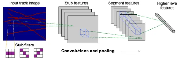
Convolutional networks are expected to be useful for pattern-recognition in track finding. Track-ing data exhibits some of the traits of natural images that are naturally exploited by convolutional networks such as translational symmetries, locality, and hierarchical multi-scale structure. In CNNs for natural images, the first convolutional layers are commonly trained to detect low-level features like edges, so it is expected that the initial layer of a CNN for tracking would identify stubs of com-patible hits in adjacent layers. Later layers of the network would then connect stub features together to form track segments, and so on until a model of an entire track or set of tracks is constructed. This conceptual model, which is useful only for intuition and may not reflect the actual learned behavior of a convolutional network, is illustrated in figure 1.
Figure 1.A possible interpretation of convolutional neural networks applied to 2D tracking data.
attention mechanisms [16–18], giving the models the capability to focus on particular parts of the input or intermediate feature representations to produce a desired output.
Such rich learned representations have also proven highly beneficial for tracking-based problems in non-HEP applications, such as sports analytics and computational neuro-science. For instance, [19] uses attention-based LSTMs to learn hierarchical models of basketball player behavior from tracking data, while [20] applies recurrent neural networks to generate realistic fruit-fly behavior and handwriting.
4 Datasets
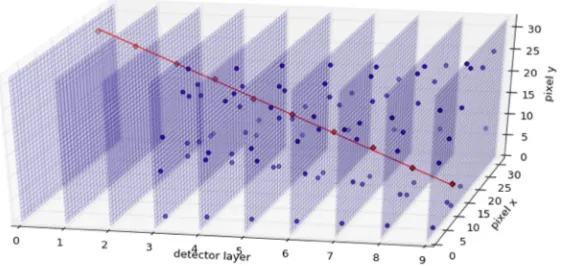
Simple toy datasets were used to study and demonstrate the ideas discussed in this paper. The "detec-tors" are made of perfect pixel planes in 2D or 3D. Tracks are sampled from straight lines contained within the detector volume, and binary hits are recorded in each intercepting discrete pixel on each layer. No trajectory curvature, material effects, or detector inefficiencies are modeled. These toy datasets are highly simplistic compared to real tracking detector data, which means that quantitative results are likely not indicative of algorithm performance in realistic scenarios. Nonetheless, this sim-ple toy data provides a useful environment to test out various models. Figure 2 shows examsim-ple 2D data generated with tracks as well as uniform noise. Figure 3 shows an example 3D event.
For the experiments described in section 5, the following data configurations were used. 2D toy experiments used one million 2D events with 50 detector layers of 50 pixels each, one signal track, and five background tracks for training. The 3D toy experiments used a detector with 10 layers and 50×50 pixels in each layer. Events were generated with a random number of background tracks sampled from a Poisson distribution with mean values varied from 1 to 100. At each point, five million events were generated for training and one hundred thousand events for testing.
5 Track finding with LSTMs and CNNs
The goal of this line of study is to identify models which can do the assignment of pixel hits to a track candidate by extrapolating from a partial track (a seed) through detector layers. When considering a single track at a time, the problem can be formulated as one of multi-class classification. The pixels in one detector layer make up the possible "classes", and the model must identify which one is traversed by the target track candidate. Modeling of track dynamics can be handled by LSTMs or CNNs.
Figure 2. 2D plane detector toy data with a configurable size, straight line tracks, and optional uniform noise hits.
Figure 3.3D plane detector toy data with ten detector layers of configurable size, straight line tracks, and optional uniform noise hits.
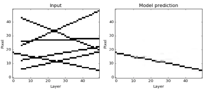
in the input by zeroing-out all non-candidate hits in the initial seed layers. Figure 5 shows an example model input and prediction after training on events with one target track and five background tracks. The simple LSTM architecture is easily able to reconstruct the target track, indicating that it can disentangle the combinatorics at each detector layer.
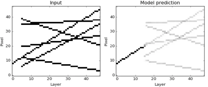
In most real tracking detectors, including those at the LHC, the number of pixels in each detector layer is not fixed and in fact increases with each successive layer. To adapt the simple rectangular image model to such a variable-sized data structure there are some options. One straightforward approach is to pad the detector image with zeros to recover the rectangular image. Another approach is to transform each pixel array through a dedicated fully connected layer to a fixed size hidden representation which is processed by the LSTM as before. In such a model, dedicated fully-connected layers on the output side of the network then transform the fixed size representation back to the target detector layer size. Figure 6 shows an example where toy data was simulated in the full rectangular detector shape but a wedge shape was cut out to demonstrate the variable-length layer model.
3 2 1 0
LSTM LSTM LSTM LSTM
FC FC FC FC
Input detector layer arrays
Target track Output detector layer
predictions
Target track 3
2 1 0
Figure 4. The basic LSTM model architecture used to classify hits for one track. The LSTM and a fully-connected layer with a softmax activation read the pixel arrays and predict which pixels belong to the target track.
Figure 5. LSTM model input (left) and prediction (right) for an example with one target track and five back-ground tracks. The first five detector layers are used to specify the target track seed. In the prediction, darker values mean greater confidence.
Figure 6.LSTM model input (left) and prediction (right) for an example with variable-sized detector layers. The white edges define the wedge detector shape as fed into the model.
Figure 7.Input and model prediction of a simple 2D convolutional model with ten convolutional layers and no down-sampling. The extrapolation of the seed track is limited in this case because the architecture does not allow to communicate information across all detector layers.
Extending the models to 3D toy detector data is mostly straightforward. For the LSTM model, all that’s required is to flatten the 2D detector layer pixel arrays into 1D arrays and proceed as before. The convolutional models need to adopt 3D convolutions. For a more detailed study of this more interesting type of toy data, we consider additional variations on the previously mentioned models. A deep-LSTM model is the same as the original LSTM model but adds additional fully-connected layers before and after the LSTM. A bidirectional LSTM model (or biLSTM) uses an additional LSTM layer which processes the detector layers in reverse order. The two LSTM outputs are concatenated before being fed into the fully connected layers for the final prediction. A next-layer LSTM model makes forward predictions on the next detector layer before reading the data on that layer.
Figure 8.A convolutional autoencoder model. Down-sampling between convolutions allows the model to con-nect information across the entire image, and up-sampling allows to recover the track of interest in the original image size.
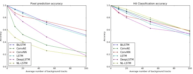
calculated in two ways: considering all pixels on each layer and considering only the pixels with hits on each layer. An example event and model predictions for the basic LSTM and the next-layer LSTM are shown in figure 10. Interestingly, the next-layer LSTM is one of the worst performers at picking the correct pixel, but is the most accurate at classifying the pixels that actually have hits. This is pre-sumed to be because the forward-thinking nature of the model gives broad, smooth track predictions that work well on straight tracks. Another interesting feature is that the convolutional models seem to scale better to high track multiplicity. Finally, none of the models perform particularly well at high track multiplicity, showing unsatisfying hit classification accuracies around 60% for 100 mean number of background tracks.
Figure 10.Example displays of a 3D toy event and model prediction for the basic LSTM (left) and the next-layer LSTM (right). The target track is shown in red. Prediction pixels are only shown for scores larger than 0.01. The basic LSTM prediction precisely follows the target hits, whereas the next-layer LSTM gives broad predictions due to it’s forward-predicting nature.
6 Track parameter estimation with LSTMs and CNNS
In addition to the hit classification models discussed in the previous section, we also considered end-to-end models that process the raw detector data without track seeds, identify tracks in the input data, and estimate the parameters of each track. The outputs of these models could be useful on their own as quantities for physics usage, or they could be used as supplementary training targets in the classification-of-hits approach.
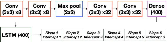
Figure 11 shows a model, built from CNNs and an LSTM, that can process a detector image and emit parameters for a variable number of tracks. In the case of the toy detector data considered here, the track parameters correspond to a line’s slope and intercept. A CNN with four layers, with a max-pooling operation between the second and third layers, is sufficient to extract relevant features from the input image. An LSTM stacked on top of the convolutional layers acts as a simple attention mechanism; it emits track parameters for each track in sequence, moving from smallest intercept value to largest. The performance of the model for events with between one and six tracks is illustrated in Figure 12, which shows the distribution of the difference between the true and predicted slope and intercept values.
Figure 11.Diagram of a model with convolutional layers followed by dense-fully-connected and LSTM layers to predict track parameters for a variable number of tracks.
per-Figure 12. Difference between true and predicted values of track slope (left) and intercept (right) for the CNN+LSTM model shown in Fig. 11. The distributions are constructed using events with up to six tracks.
formance, the model is trained by maximizing the following log gaussian likelihood, which relates the true track parametersy, their predicted values f(x), and the covariance matrix Σoutput by the network:
L(x, y)=log|Σ|+(y−f(x))TΣ−1(y−f(x)) (1)
Figure 13 illustrates the predicted track parameters and their uncertainties for an example event with six tracks.
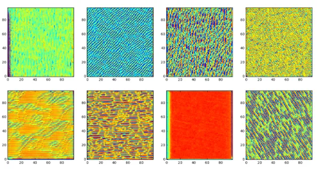
The convolutional filters learned by the model provide insight into the features that the model has learned to extract. A filter can be visualized by using gradient ascent to find an input image that max-imizes the filter’s output activation [21]. Using this technique we generated the images shown in fig-ure 14, which provide visualization of the filters in the second convolutional layer of the CNN+LSTM model.
Figure 14.Visualization of the CNN+LSTM model’s second layer filters via gradient ascent optimization of the inputs.
7 Conclusion
In this paper we have prototyped and demonstrated some preliminary ideas for adopting machine learning techniques for particle tracking problems. This is still a relatively unexplored space and we have only just begun to scratch the surface, but nonetheless some of the technologies used in the field of deep learning show some promise in this field as well. LSTMs were seen to be effective at the problem of hit assignment in 2D and 3D with a sequence of detector layer measurements and may be viable as an alternative to the combinatorial Kalman Filter. CNNs were shown to be able to construct representations of the detector data in a ground-up fashion that are useful for hit assignment or parameter and uncertainty estimation. By attaching an LSTM to a CNN model we demonstrated a potentially powerful end-to-end model which can find a variable number of tracks in a detector image. All of the explored models were trained and tested on GPUs, demonstrating parallelization capabilities that help to address the scaling issues of traditional tracking algorithms.
There are numerous clear hurdles to adopt these methods in realistic scenarios. Real particle detectors are typically irregular in layout and may not be easily transcribed into the image format. The high granularity and sparsity of real detector data poses a dimensionality and scaling problem for solutions that work in discrete spaces.
All models studied in this paper were implemented in the Keras [23] framework. The code with full details of the models and training in Jupyter notebooks is available at [24].
The authors would like to thank the funding agencies DOE ASCR and COMP HEP for supporting this work, as well as the numerous tracking experts from ATLAS and CMS who have shared insights and experience.
References
[1] L. Evans, P. Bryant, JINST3, S08001 (2008) [2] G. Aad et al. (ATLAS), JINST3, S08003 (2008) [3] S. Chatrchyan et al. (CMS), JINST3, S08004 (2008) [4] B. Schmidt, J. Phys. Conf. Ser.706, 022002 (2016) [5] Y. LeCun, Y. Bengio, G. Hinton, Nature521, 436 (2015)
[6] I. Goodfellow, Y. Bengio, A. Courville,Deep learning(MIT Press, 2016)
[7] R. Fruehwirth, M. Regler, R. Bock, H. Grote, D. Notz, Data Analysis Techniques for High-Energy Physics, 2nd edn. (Cambridge University Press, Cambridge UK, 2000)
[8] F. Ragusa, L. Rolandi, New Journal of Physics9, 336 (2007)
[9] R. Frühwirth, A. Strandlie, Pattern recognition and reconstruction: Datasheet from landolt-börnstein - group i elementary particles, nuclei and atoms · volume 21b1: “detec-tors for particles and radiation. part 1: Principles and methods” in springermaterials (http://dx.doi.org/10.1007/978-3-642-03606-4_13), copyright 2011 Springer-Verlag Berlin Hei-delberg,http://materials.springer.com/lb/docs/sm_lbs_978-3-642-03606-4_13 [10] The ATLAS Collaboration,The Optimization of ATLAS Track Reconstruction in Dense
Environ-ments(2015),https://cds.cern.ch/record/2002609
[11] A. Salzburger, Tracking at HL-LHC and FCC (2015),
https://indico.hephy.oeaw.ac.at/event/86/session/2/contribution/4
[12] R. Mankel, Nuclear Instruments and Methods in Physics Research Section A: Accelerators, Spectrometers, Detectors and Associated Equipment395, 169 (1997)
[13] S. Levine, C. Finn, T. Darrell, P. Abbeel, arXiv preprint arXiv:1504.00702 (2015) [14] S. Hochreiter, J. Schmidhuber, Neural Comput.9, 1735 (1997)
[15] O. Vinyals, A. Toshev, S. Bengio, D. Erhan, CoRRabs/1411.4555(2014) [16] M. Denil, L. Bazzani, H. Larochelle, N. de Freitas, CoRRabs/1109.3737(2011) [17] V. Mnih, N. Heess, A. Graves, K. Kavukcuoglu, CoRRabs/1406.6247(2014)
[18] K. Xu, J. Ba, R. Kiros, K. Cho, A.C. Courville, R. Salakhutdinov, R.S. Zemel, Y. Bengio, CoRR abs/1502.03044(2015)
[19] S. Zheng, Y. Yue, J. Hobbs,Generating Long-term Trajectories Using Deep Hierarchical Net-works, inAdvances in Neural Information Processing Systems(2016), pp. 1543–1551
[20] E. Eyjolfsdottir, K. Branson, Y. Yue, P. Perona, arXiv preprint arXiv:1611.00094 (2016) [21] K. Simonyan, A. Vedaldi, A. Zisserman, CoRRabs/1312.6034(2013)
[22] A Common Tracking Software Project,http://acts.web.cern.ch/ACTS/index.php [23] F. Chollet et al.,Keras, https://github.com/fchollet/keras (2015)