Evaluation of the RPC Model for Ziyuan-3 Three-line Array Imagery
Zhonghua Hong 1,*, Shengyuan Xu 1, Yun Zhang 1,*, Yanling Han 1 and Yongjiu Feng 2
1 College of Information Technology, Shanghai Ocean University, 999 Hu-Chenghuan Road, Shanghai 201306, P. R. China. 2 College of Marine Science, Shanghai Ocean University, 999 Hu-Chenghuan Road, Shanghai 201306, P. R. China.
* Correspondence: [email protected]; [email protected]
Abstract: Ziyuan-3 (ZY-3) satellite is the first civilian stereo mapping satellite in China and was designed to achieve the 1: 50000 scale mapping for land and ocean. Rigorous sensor model (RSM) is required to build the relationship between the three-dimensional (3D) object space and two-dimensional (2D) image space of ZY-3 satellite imagery. However, each satellite sensor has its own imaging system with different physical sensor models, which increase the difficulty of geometric integration of multi-source images with different sensor models. Therefore, it is critical to generate generic model, especially rational polynomial coefficients (RPCs) of optical imagery. Recently, relatively a few researches have been conducted on RPCs generation to ZY-3 satellite. This paper proposes an approach to evaluate the performance of RPCs generation from RSM of ZY-3 imagery. Three scenarios experiments with different terrain features (such as ocean, city and grassland) are designed and conducted to comprehensively evaluate the replacement accuracies of this approach and analyze the RPCs fitting error. All the experimental results demonstrate that the proposed method achieved the encouraging accuracy of better than 1.946E-04 pixel in both x-axis direction and y-axis direction, and it indicates that the RPCs is suitable for ZY-3 imagery and can be used as a replacement for the RSM of ZY-3 imagery.
Keywords: rational polynomial coefficients (RPCs); ziyuan-3 satellite; rigorous sensor model (RSM)
1. Introduction
High resolution satellite imagery (HRSI) becomes a large source of area information. Remote sensing technology has played a more and more important role in Earth observation. Crucial to land and ocean mapping, sensor model of HRSI is typically divided into two categories, namely the rigorous sensor models (RSMs) and generalized models (GL) (Poli and Toutin, 2012). The RSMs of space-borne linear array charge-coupled device (CCD) optical imagery is mainly based on linear array co-linearity equation according with interior orientation (IO) and exterior orientation (EO) parameters of imagery (Poli 2015; Jannati et al., 2017). However, each satellite sensor has its own imaging system with various RSMs which increase the difficulty of developing geometric processing software that is capable of handling multi-source remote sensing data. Therefore, developing a replacement sensor model independent of sensor platforms and sensor types becomes attractive for processing of new satellite sensor (Toutin 2004; Eftekhari et al., 2013). The rational function model (RFM) is the ratio of two cubic polynomials with 78 rational polynomial coefficients (RPCs) has been reported as an alternative sensor orientation model for high-resolution satellite imagery (HRSI) (Fraser et al., 2005), such as IKONOS, Quickbird, GeoEye-1 and WorldView-2, etc (Dial et al., 2003; Fraser et al., 2003, 2005, 2006, 2009; Grodecki and Dial, 2003; Li et al., 2007, 2008; Tong et al., 2010, 2012). At the same time, several researchers focus on non-ground control points based on compensation models for reducing the bias error of vendor-provided RPCs (Naeini et al., 2018; Yavari et al., 2018; Noh and Howat, 2018). Therefore, the accuracy of RPC generation is very important to newly launched satellite.
This paper presents an approach to generate the RPCs for ZY-3 imagery from RSM. Three scenarios experiments with different terrain features (such as grassland, hill, city and ocean) are designed and conducted to comprehensively evaluate the replacement accuracies of this approach and analyze the RPCs fitting error.
2. Methodology
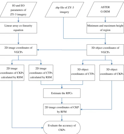
Figure 1. Framework for RPCs generation of ZY-3 imagery.
2.1. RSM of ZY-3 imagery based on linear array co-linearity equation
The scanning mode of ZY-3 imagery is push-broom linear CCD, i.e. which is scanned along the flight direction (Tang et al., 2015). To assume that the flight direction is in line with x-axis direction as coordinates x direction, and scan line direction in line with y-axis direction as the coordinate y direction, the sensor model can be written as following:
IO and EO parameters of ZY-3 imagery
ASTER G-DEM
Linear array co-linearity equation
Minimum and maximum height of region
3D object coordinates of VGCPs
.shp file of ZY-3 imagery
2D image coordinates of VGCPs
2D image coordinates of CKPs
calculated by RSM
Estimate the RPCs 2D image
coordinates of CTPs calculated by RSM
3D object coordinates of CTPs
3D object coordinates of CKPs
2D image coordinates of CKP by RFM
1 ) tan( ) tan( ) ( ) ( ) ( ) ( ) ( 2000 84 2000 84 84 X Y Body Camera z y x z y x Orbit Body J Orbit WGS J WGS S S S WGS P P P f R d d d D D D R t R t R m t Z t Y t X Z Y X (1)
Where, (XS(t), YS(t), ZS(t)) and (XP, YP, ZP) are the perspective center coordinates and
object coordinates in the WGS84 coordinate system, respectively. m denotes the scaling factor, f is the focal length of the satellite camera. (RBodyOrbit,ROrbitJ2000(t),RWGSJ200084(t)) are the rotation matrices from the satellite body system to satellite orbit system, J2000 coordinate system and WGS84 coordinate system, respectively. (Dx, Dy, Dz) and (dx, dy, dz) are the displacement of the phase center and CCD array center of the satellite body, respectively. RCameraBody represents the rotation matrix from the satellite camera coordinate system to the body coordinate system. (X,Y) denotes the look angle. Meanwhile,RCameraBody
were measured before the satellite launch.
Rotation angles and perspective center coordinate can be interpolated using second-order polynomials with time t. Furthermore, the relationship between the look angle and image coordinates (
x,y) can be expressed as following:
1 ) tan( ) tan( 0 0 X Y f f y y x x (2)
Where, (x0,y0) are the image coordinates of the principal point.
At last, replacing the tan(X) and tan(Y) in Equation 1 by the xx0 and yy0 in Equation 2 and the reverse form of the Equation 1, which transforms from the object space to image space, can be expressed as:
Where, aij (i1,2,3; j1,2,3) are elements of the rotation matrix from body coordinate system to the geocentric Cartesian coordinate system.
2.2. RFM of high resolution satellite imagery
RFM (Tao and Hu, 2001) performs the same transformation through a generalized version of polynomials, and a ratio of two polynomials, which is similar as co-linearity equation. The RFM can be expressed as following:
) , , ( ) , , ( 2 1 W V U P W V U P r ) , , ( ) , , ( 4 3 W V U P W V U P
c (4)
Where, (r, c) are the normalized image coordinates to the range from -1.0 to 1.0 by their image size, (U , V , W) are the normalized ground coordinates to the range from -1.0 to 1.0 by their geometric extend. Pi(U,V,W) (i= 1, 2, 3 and 4) are the polynomial.
Usually, the order of the polynomials is limited by 0m13, 0m23, 0m33 and m1+m2+m33. Each Pi(U,V,W) (i= 1, 2, 3 and 4) is then a third order twenty-term polynomial:
3 19 3 18 3 17 2 16 2 15 2 14 2 13 2 12 2 11 10 2 9 2 8 2 7 6 5 4 3 2 1 0 ) , , ( W a V a U a VW a UW a W V a UV a W U a V U a UVW a W a V a U a VW a UW a UV a W a V a U a a W V U Pi (5)
If equation (4) is substituted in Equation (3) and eliminated the first coefficient in the denominator, the RFM becomes:
T T T T d d d W V U W V U c c c c W V U W V U c b b b W V U W V U a a a a W V U W V U r ) , , , , 1 )( , , , , , , , 1 ( ) , , , , )( , , , , , , , 1 ( ) , , , , 1 )( , , , , , , , 1 ( ) , , , , )( , , , , , , , 1 ( 19 2 1 3 3 3 19 2 1 0 3 3 3 19 2 1 3 3 3 19 2 1 0 3 3 3 (6)
Where,ai (i=0,
, 19) are RPCs.
2.3. RPC generation of ZY-3 imagery
The virtual grid corresponding points (VGCPs) were generated to estimate the RPCs by employing the terrain-independent approach (Tao and Hu, 2001; Fraser et al., 2006), which depends upon the RSM of ZY-3 imagery. Terrain-independent approach was used to generate the VGCPs from object space to image space. This conversion includes three steps as following:
(1) The object space was divided into m × n grids in the first step;
(2) And then, the corresponding elevation of object grid points can be obtained from the ASTER G-DEM (30m) covering the full extent of the image;
(3) To calculate the image grid coordinates of corresponding object grid points in accordance with the linear array co-linearity Equation 3 using VGCPs in image space for ZY-3 imagery.
And then, half VGCPs were selected as CTPs to estimate the RPCs. At the same time, the remaining half VGCPs as CKPs were used to evaluate the RPC generation accuracy.
2.3.2. RPCs estimation
The 78 unknown RPCs are then can be estimated by least squares adjustment according by the CTPs selected from the generated VGCPs by method introduced in Section 2.3.1.
After linearlizing from the Equation 6, we have:
c d d c c c cW cU W U v D r b b a a a rW rU W U v D T c T r 19 1 19 1 0 3 3 2 19 1 19 1 0 3 3 1 , , , , , , , , , , , , 1 , , , , , , , , , , , , 1 (7) Where,
T T b b b W V U W V U D d d d W V U W V U D 19 2 1 3 3 3 2 19 2 1 3 3 3 1 , , , , 1 , , , , , , 1 , , , , 1 , , , , , , 1 (8)Since there are 78 unknown coefficients in Equation 8, more than 39 CTPs with known image and ground coordinates are needed to have a least squares solution.
The above observation equation can also be expressed in matrix form as:
L AX
V (9) Its least squares solution is
) ( ) ( ˆ 1 L A A A
2.3.3. RPCs validation
The RPCs validation includes three steps as following:
(1) In the first step, selecting another half VGCPs as CKPs used to generate the VGCPs accordance with RSM of ZY-3 imagery as introduced in Section 2.3.1;
(2) And then, calculating the 2D image coordinates of CKPs selected from the generated 3D object coordinates of VGCPs according to the generated RPCs introduced in Section 2.3.2.
(3) At last, the accuracy of the RPCs generation can be evaluated by calculating the difference between the 2D image coordinates of the CKPs calculated from the generated RPCs and 2D image coordinates of the CKPs from the RSM.
3. Experiments and discussion
3.1. Study area and data sources
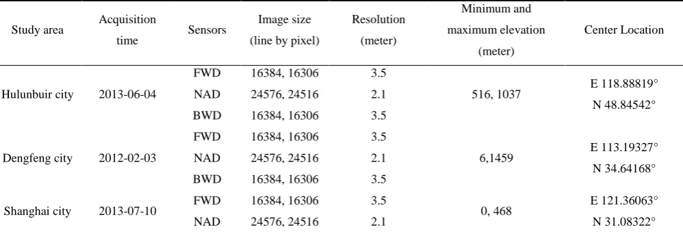
We performed a comprehensive experiment to test the potential of RPC generation for ZY-3 imagery using three data sets in the ocean region, city region and grassland region, respectively. Figure 2 shows the three study areas (Hulunbuir City, Dengfeng City, Shanghai City and Sansha City, China) and scenes with NAD, FWD and BWD images of ZY-3 satellite. Table 1 presents the detailed information about these images used in the experiment, comprising the acquisition time, sensor name, image size, resolution, minimum/maximum elevation and center location.
Table 1. Image information of ZY-3 images from the three study areas
Study area Acquisition
time Sensors
Image size
(line by pixel)
Resolution
(meter)
Minimum and
maximum elevation
(meter)
Center Location
Hulunbuir city 2013-06-04
FWD
NAD
BWD
16384, 16306
24576, 24516
16384, 16306
3.5
2.1
3.5
516, 1037 E 118.88819° N 48.84542°
Dengfeng city 2012-02-03
FWD
NAD
BWD
16384, 16306
24576, 24516
16384, 16306
3.5
2.1
3.5
6,1459 E 113.19327°
N 34.64168°
Shanghai city 2013-07-10 FWD NAD
16384, 16306
24576, 24516
3.5
2.1 0, 468
E 121.36063°
BWD 16384, 16306 3.5
Sansha city 2013-05-01
FWD
NAD
BWD
16384, 16306
24576, 24516
16384, 16306
3.5
2.1
3.5
0, 16 E 112.41435°
N 16.76861°
Figure 2. The three study areas and scenes with NAD, FWD and BWD images of ZY-3 satellite. In the experiments, RPCs generation for ZY-3 imagery, as introduced in Section 2.3, was conducted for three data sets. To evaluate the accuracy and reliability of the proposed method, the experiments have been designed as four aspects. The first aspect is comparing the performance of RPC generation with different terrain features (such as: Ocean Region (Sansha City), hilly region (Dengfeng
NAD
NAD
NAD
FWD
FWD
FWD
BWD
BWD
BWD (a) ZY-3 NAD, FWD and BWD images in study area of Hulunbuir city
(c) ZY-3 NAD, FWD and BWD images in study area of Shanghai city
(d) ZY-3 NAD, FWD and BWD images in study area of Sansha city (b) ZY-3 NAD, FWD and BWD images in study area of Dengfeng city
City) city region (Shanghai City) and grassland region (Hulunbuir City)). The second aspect is comparing the performance of RPC generation with different sensors (such as: FWD camera, NAD camera and BWD camera). The third aspect is evaluating the influence on the size of the VGCPs’ grid. The fourth aspect is evaluating the influence on the number of the VGCPs’ height layers.
To ensure adequate number of observations, the minimum size of VGCPs is defined as 10 × 10 (10 lines by 10 samples in a horizontal plane) with at least 3 elevation layers, These scenarios are using different sizes from 10 × 10 to 30 × 30 in line and sample direction and different sizes from 3 to 10 in elevation direction to evaluate the performance of different sizes of VGCPs.
3.2. Comparison of the performance of RPCs generation with different terrain features
Figure 3. Accuracy of RPCs generation for ZY-3 image in Shanghai study region.
Figure 4. Accuracy of RPCs generation for ZY-3 image in Dengfeng study region. 0.00000
0.00005 0.00010 0.00015 0.00020
Ac
cu
rac
y
(pixel)
Grid size
RMS error in x direction (NAD) RMS error in y direction (NAD) RMS error in x direction (FWD) RMS error in y direction (FWD) RMS error in x direction (BWD) RMS error in y direction (BWD)
0.00000 0.00005 0.00010 0.00015 0.00020
Acc
ura
cy
(
pix
el)
Grid size
Figure 5. Accuracy of RPCs generation for ZY-3 image in Sansha study region.
Figure 6. Accuracy of RPCs generation for ZY-3 image in Hulunbuir study region.
3.2. Comparison of the performance of RPCs generation with different sensor image
0.00000 0.00005 0.00010 0.00015 0.00020
Acc
ura
cy
(
pix
el)
Grid size
RMS error in x direction (NAD) RMS error in y direction (NAD) RMS error in x direction (FWD) RMS error in y direction (FWD) RMS error in x direction (BWD) RMS error in y direction (BWD)
0.00000 0.00005 0.00010 0.00015 0.00020
Acc
ura
cy
(
pix
el)
Grid size
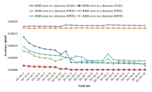
Figure 7 and Figure 8 show the comparison of the performance of RPCs generation for ZY-3 FWD-NAD-BWD imageries in x direction and y direction with 10 × 10 in line and sample direction and different sizes from 3 to 10 in elevation direction, respectively. As can be seen from Figure 7 and Figure 8, the accuracy of RPC fitting for ZY-3 BWD imagery is better than FWD imagery and NAD imagery in x direction. At the same time, the FWD imagery and BWD imagery have a reasonable consistency and similar trend in y direction.
(a) FWD sensor 0.00000
0.00002 0.00004 0.00006 0.00008 0.00010 0.00012 0.00014 0.00016 0.00018 0.00020
10×10×3 10×10×4 10×10×5 10×10×6 10×10×7 10×10×8 10×10×9 10×10×10
Acc
ura
cy
(
pix
el)
Grid size
(b) NAD sensor
(c) BWD sensor
Figure 7. Accuracy of RPCs generation for ZY-3 FWD-NAD-BWD images in x direction. 0.00000
0.00005 0.00010 0.00015 0.00020
10×10×3 10×10×4 10×10×5 10×10×6 10×10×7 10×10×8 10×10×9 10×10×10
Acc
ura
cy
(
pix
el)
Grid size
RMS error in x direction in Shanghai region (NID) RMS error in x direction in Sansha region(NID) RMS error in x direction in Hulunbuir region (NID) RMS error in x direction in Dengfeng region (NID)
0.00000 0.00005 0.00010 0.00015 0.00020
10×10×3 10×10×4 10×10×5 10×10×6 10×10×7 10×10×8 10×10×9 10×10×10
Acc
ura
cy
(
pix
el)
Grid size
(a) FWD sensor
(b) NAD sensor 0.00000
0.00005 0.00010 0.00015 0.00020
10×10×3 10×10×4 10×10×5 10×10×6 10×10×7 10×10×8 10×10×9 10×10×10
A
cc
ur
a
cy
(
pixel
)
Grid size
RMS error in y direction in Shanghai region (FWD) RMS error in y direction in Sansha region (FWD) RMS error in y direction in Hulunbuir region (FWD) RMS error in y direction Dengfeng region (FWD)
0.00000 0.00002 0.00004 0.00006 0.00008 0.00010 0.00012 0.00014 0.00016 0.00018 0.00020
10×10×3 10×10×4 10×10×5 10×10×6 10×10×7 10×10×8 10×10×9 10×10×10
Acc
ura
cy
(
pix
el)
Grid size
(c) BWD sensor
Figure 8. Accuracy of RPCs generation for ZY-3 FWD-NAD-BWD images in y direction.
3.3. Comparison of the performance of RPCs generation with different height layers
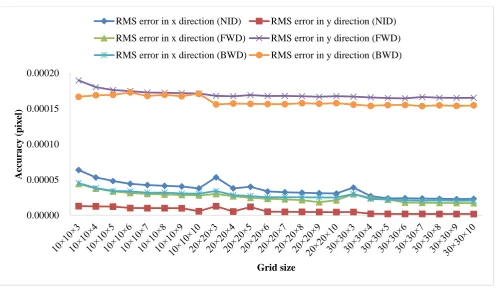
In order to evaluate the influence of the height layer on the RPC accuracy, 3D control grids consisting of 10×10 grid each with height layer from 3 to 10 were established. Figure 9 shows the comparison of the different height layers’ performance in three study regions in x-axis direction and y-axis direction, respectively. From the tests’ results, it can be seen obviously that the RMS error of CKPs is reducing as the height layer increases in all test data sets in x direction. Meanwhile, the RMS error of the CKPs will not be improved much once the height layer increases in y-axis direction, which means that using a denser grid would not be beneficial to the accuracy.
0.00000 0.00005 0.00010 0.00015 0.00020
10×10×3 10×10×4 10×10×5 10×10×6 10×10×7 10×10×8 10×10×9 10×10×10
Acc
ura
cy
(
pix
el)
Grid size
(a) x-axis direction 0.00000
0.00005 0.00010 0.00015 0.00020
3 4 5 6 7 8 9 10
Acc
ura
cy
(
pix
el)
Height layer
(b) y-axis direction
Figure 9. The accuracy of the CKPs with the height layer on ZY-3 three-line array imageries in both x-axis direction and y-axis direction.
0.00000 0.00005 0.00010 0.00015 0.00020
3 4 5 6 7 8 9 10
A
cc
ur
a
cy
(
pixel
)
Height layer
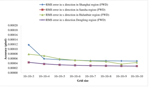
3.4. Comparison of the performance of RPCs generation with different grid sizes
(a) x-axis direction
0.000E+00 2.000E-05 4.000E-05 6.000E-05 8.000E-05 1.000E-04 1.200E-04 1.400E-04 1.600E-04
10×10×3 20×20×3 30×30×3
A
ccuracy
()
pi
xel
Grid layers
RMS error in x direction in Shanghai region (NID)
RMS error in x direction in Shanghai region (FWD)
RMS error in x direction in Shanghai region (BWD)
RMS error in x direction in Sansha region (NID)
RMS error in x direction in Sansha region (FWD)
RMS error in x direction in Sansha region (BWD)
RMS error in x direction in Hulunbuir region (NID)
RMS error in x direction in Hulunbuir region (FWD)
RMS error in x direction in Hulunbuir region (BWD)
RMS error in x direction in Dengfeng region(NID)
RMS error in x direction in Dengfeng region(FWD)
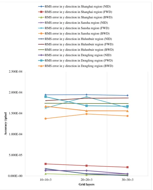
(b) y-axis direction
Figure 10. The accuracy of the CKPs with the grid number on ZY-3 three-line array imageries in both x-axis direction and y-axis direction.
4. Conclusion
0.000E+00 5.000E-05 1.000E-04 1.500E-04 2.000E-04 2.500E-04
10×10×3 20×20×3 30×30×3
A
ccuracy
()
pi
xel
Grid layers
RMS error in y direction in Shanghai region (NID)
RMS error in y direction in Shanghai region (FWD)
RMS error in y direction in Shanghai region (BWD)
RMS error in y direction in Sansha region (NID)
RMS error in y direction in Sansha region (FWD)
RMS error in y direction in Sansha region (BWD)
RMS error in y direction in Hulunbuir region (NID)
RMS error in y direction in Hulunbuir region (FWD)
RMS error in y direction in Hulunbuir region (BWD)
RMS error in y direction in Dengfeng region (NID)
RMS error in y direction in Dengfeng region (FWD)
This paper has presented a RPCs generation model for Ziyuan-3 stereo survey satellite. The results of comparison experiment in Hulunbuir City, Dengfeng City, Shanghai City and Sansha City proved our method’s feasibility and effectiveness for ZY-3 three-line imageries. Based on four scenarios experiments with different terrain features (such as ocean, hill, city and grassland), several conclusions are drawn as follows:
(1) By use of presented RPC generation method for ZY-3 three-line imageries, the fitting model performed very well in ocean region, hilly region, city region and grassland region, and achieved the encouraging accuracy of better than 1.946E-04 pixel in both x-axis direction and y-axis direction, and it revealed that RFM can be widely used to replace the RSM for ZY-3 three-line imageries.
(2) The performance of RPCs generation model for the ZY-3 BWD imagery is better than FWD imagery and NAD imagery in x-axis direction. At the same time, the FWD imagery and BWD imagery have a reasonable consistency and the similar trend in y-axis direction.
(3) The accuracy of RPCs fitting for ZY-3 three-line imageries is improving as the height layers increase in test data sets in x-axis direction. However, the layers increases will be not beneficial to the accuracy of RPCs fitting when height layers increase in y-axis direction.
References
1. Chen, Y.; Xie, Z.; Qiu, Z.; Zhang, Q.; Hu, Z. Calibration and validation of ZY-3 optical sensors. IEEE Trans. Geosci. Remote Sens.2015, 53(8), 4616-4626.
2. Dial, G., Bowen, H., Gerlach, F., Grodecki, J., Oleszczuk, R. IKONOS satellite, imagery, and products. Remote Sens Environ, 2003,88(1), 23-36.
3. Eftekhari, A., Saadatseresht, M., Motagh, M. A study on rational function model generation for TerraSAR-X imagery. Sensors, 2013, 13(9), 12030-12043.
4. Fraser, C.S.; Hanley, H.B. Bias compensation in rational functions for Ikonos satellite imagery. Photogramm. Remote Sens. 2003, 69, 53-57.
5. Fraser, C.S.; Hanley, H.B. Bias-compensated RFMs for sensor orientation of high-resolution satellite imagery. Photogramm. Remote Sens. 2005, 71, 909-915.
6. Fraser, C.S.; Dial, G.; Grodecki, J. Sensor orientation via RPCs. ISPRS J. Photogramm. Remote Sens.2006, 60, 182-194.
7. Fraser, C.S.; Ravanbakhsh, M. Georeferencing accuracy of GeoEye-1 imagery. Photogramm. Remote Sens. 2009, 75, 634-638.
8. Grodecki, J.; Dial, G. Block adjustment of high-resolution satellite images described by rational polynomials. Photogramm. Eng. Remote Sens.2003, 69, 59–68.
9. Jannati, M., Valadan Zoej, M. J., Mokhtarzade, M. Epipolar Resampling of Cross-Track Pushbroom Satellite Imagery Using the Rigorous Sensor Model. Sensors, 2017, 17(1), 129,1-19. 10. Li, R.; Zhou, F.; Niu, X.; Di, K. Integration of IKONOS and QuickBird imagery for
geopositioning accuracy analysis. Photogramm. Remote Sens. 2007, 73, 1067-1074.
11. Li, R.; Deshpande, S.; Niu, X.; Zhou, F.; Di, K.; Wu, B. Geometric integration of aerial and high-resolution satellite imagery and application in shoreline mapping. Mar Geod. 2008, 31, 143-159.
Optimization of Terrain-Independent RFMs for VHSR Satellite Images. IEEE Geosci Remote S.
2017, 14(8):1368-72.
13. Noh M.J., Howat I.M. Automatic relative RPC image model bias compensation through hierarchical image matching for improving DEM quality. ISPRS J. Photogramm. Remote Sens. 2018, 136:120-133.
14. Poli, D. A rigorous model for spaceborne linear array sensors. Photogramm. Remote Sens. 2007, 73, 187-196.
15. Poli, D., Toutin, T. Review of developments in geometric modelling for high resolution satellite pushbroom sensors. Photogramm Rec, 2012, 27(137), 58-73.
16. Poli D, Remondino F, Angiuli E, Agugiaro, G. Radiometric and geometric evaluation of GeoEye-1, WorldView-2 and Pléiades-1A stereo images for 3D information extraction. ISPRS J. Photogramm. Remote Sens, 2015, 100, 35-47.
17. Tang, X., Zhou, P., Zhang, G., Wang, X., Pan, H. Geometric accuracy analysis model of the ZiYuan-3 satellite without GCPs. Photogramm. Remote Sens, 2015, 81(12), 927-934.
18. Tao, C.V.; Hu, Y. A comprehensive study of the rational function model for photogrammetric processing. Photogramm. Remote Sens. 2001, 67, 1347-1357.
19. Toutin, T. Review article: geometric processing of remote sensing images: models, algorithms and methods. INT J Remote Sen.2004, 25, 1893-1924.
20. Tong, X.H.; Liu, S.J.; Weng, Q.H. Bias-corrected rational polynomial coefficients for high accuracy geo-positioning of QuickBird stereo imagry. ISPRS J. Photogramm. Remote Sens. 2010,
65, 218-226.
21. Tong, X.H.; Hong, Z.H.; Liu, S.J; Zhang, X.; Xie, H.; Li, Z.Y.; Yang, S.L.; Wang, W.A.; Bao, F. Building-damage detection using pre- and post-seismic high-resolution IKONOS satellite stereo imagery: a case study of the May 2008 Wenchuan Earthquake. ISPRS J. Photogramm. Remote Sens. 2012, 68, 13-27.
detection of the ZY-3 satellite by using multispectral parallax images. IEEE Trans. Geosci. Remote Sens, 2015, 53(6), 3522-3534.
23. Yavari, S., Valadan Zoej M.J,, Sahebi M.R., Mokhtarzade M. Accuracy improvement of high resolution satellite image georeferencing using an optimized line-based rational function model.