Computing Four-Center Two-Electron Coulomb Integrals Using Exponential Transformations and Trapezoidal Rule

(1)

Computing Four-Center Two-Electron Coulomb Integrals

Using Exponential Transformations and Trapezoidal Rule

JordanLovrod1,_and _Hassan_Safouhi1, 1_{Campus Saint-Jean, University of Alberta,}

8406, 91 Street, Edmonton, Alberta T6C 4G9, Canada

Abstract. The numerical evaluations of the four-center two-electron Coulomb inte-grals are among the most time-consuming computations involved in molecular elec-tronic structure calculations. In the present paper we extend the double exponential (DE) transform method, previously developed for the numerical evaluation of three-center one-electron molecular integrals [J. Lovrod, H. Safouhi, Molecular Physics (2019)

DOI:10.1030/0026867.2019.1619854], to four-center two-electron integrals. The fast convergence properties analyzed in the numerical section illustrate the advantages of the new approach.

1 Introduction

The double exponential (DE) transformation method for the numerical evaluation of three-center one-electron molecular integrals [1] is extended in the present paper for the evaluation of the notoriously difficult four-center molecular integrals.

The analytical expression of a four-center molecular integral, which can be derived via the Fourier transform method, contains a semi-infinite integralJ(s,t), the integrand of which is slowly decay-ing and involves the spherical Bessel function jλ(vx). In particular, whenλand/orvare large, the

oscillations of the integrand can become huge, thus complicating the accurate approximation of the integral by any of the existing numerical programming platforms. By applying theS transformation [2] followed by the DE transformation [1], we obtain a bi-infinite integral, which can be approximated by a trapezoidal rule. Relatively few collocation points were required in order to obtain accurate ap-proximations.

2 General definitions and properties

The spherical Bessel function jλ(x) of orderλ∈N0, [3, 4], is given by

jλ(x) = (−1)λxλ

d xdx

λ

j0(x) = (₋1)λxλ

d xdx

λ

sinx x

. (1)

(2)

The reduced Bessel function ˆkn+1

2(z) with half-integral order [5, 6] is given by

ˆ kn+1

2(z) =

2

πz

n+1 2K

n+1 2(z) = z

n_e−z n j=0

(n+j)!

j! (n−j)! 1

(2z)j, (2)

wheren∈N, and whereKn+1

2(z) is the modified Bessel function of the second kind [7].

TheBfunctions [6, 8] are defined by

Bm

n,l(ζ,#—r)= (

ζr)l 2n+l₍_n₊_l_)!kˆn−1

2(ζr)Y

m

l (θ#—_r, ϕ#—_r), (3)

wheren,l,mare the quantum numbers, Ym

l (θ, ϕ) denotes the surface spherical harmonic, which is defined using the Condon-Shortley phase convention [9] andPm

l (x) is the associated Legendre poly-nomial of thelth degree andmth order.

The Fourier transform ¯Bm n,l(ζ,

#—

p) ofBm n,l(ζ,

#—

r) (3) is given by [10]:

¯ Bm

n,l=

2

πζ

2n+l−1 (−ip)l (ζ2+p2)n+l+1Y

m

l (θ#—_p, ϕ#—_p). (4)

The four center two-electron Coulomb integrals are given by:

Jn2l2m2,n4l4m4

n1l1m1,n3l3m3 =

#—

R,#—R

Bm1

n1,l1

ζ1,

#—

R−OA# —∗Bm3

n3,l3

ζ3,

#—

R₋# —

OC∗ 1

#—

R−#—R

× Bm2

n2,l2

ζ2,

#—

R −OB# —Bm4

n4,l4

ζ4,

#—

R₋# —

ODd#—Rd#—R_, ₍₅₎

wheren,landmare the quantum numbers,A,B,CandDare arbitrary points in the Euclidean space, andOstands for the origin of the fixed coordinate system.

In the case whereA=C, we obtain the expression of three-center exchange integrals. Two-center exchange integrals correspond to the case whereA=CandB=D.

By performing the translations of vectorsOA# —andOD# —, we can write the four center two-electron Coulomb integrals as follows:

Jn2l2m2

n1l1m1,n3l3m3(ζ1, ζ2, ζ3, ζ4,

#—

R21,

#—

R31,

#—

R34) = Bmn11,l1(ζ1,

#—

r)∗Bm3

n3,l3(ζ3,

#—

r₋#—

R34)

∗

× 1

#—

r −#—

r₋#—_R₃₁B

m2

n2,l2(ζ2,

#—

r −#—R21)Bm4

n4,l4(ζ4,

#—

r_{) d}#—

rd#—

r_. ₍₆₎

where#—

r =#—R−OA# —, #—r=#—R−OD# —, R#—12 =BA# —, #—R31 =AC# —and#—R34=DC# —.

3 Four-center two-electron Coulomb integrals

The analytical expression of the four-center two-electron Coulomb integrals in terms ofBfunctions can be derived via the Fourier transform method [11, 12]. The problematic semi-infinite oscillatory integral involved in the obtained analytical expression is given by:

J(s,t)=

∞

0 x

nxkˆν12

_R

21γ12(s,x)

_γ

12(s,x)nγ12 ˆ kν34

_R

34γ34(t,x)

(3)

The reduced Bessel function ˆkn+1

2(z) with half-integral order [5, 6] is given by

ˆ kn+1

2(z) =

2 πz n+1 2K n+1 2(z) = z

n_e−z n j=0

(n+ j)!

j! (n−j)! 1

(2z)j, (2)

wheren∈N, and whereKn+1

2(z) is the modified Bessel function of the second kind [7].

TheBfunctions [6, 8] are defined by

Bm

n,l(ζ,#—r)= (

ζr)l 2n+l₍_n₊_l_)!kˆn−1

2(ζr)Y

m

l (θ#—_r, ϕ#—_r), (3)

wheren,l, mare the quantum numbers, Ym

l (θ, ϕ) denotes the surface spherical harmonic, which is defined using the Condon-Shortley phase convention [9] andPm

l(x) is the associated Legendre poly-nomial of thelth degree andmth order.

The Fourier transform ¯Bm n,l(ζ,

#—

p) ofBm n,l(ζ,

#—

r) (3) is given by [10]:

¯ Bm

n,l=

2

πζ

2n+l−1 (−ip)l (ζ2+p2)n+l+1Y

m

l (θ#—_p, ϕ#—_p). (4)

The four center two-electron Coulomb integrals are given by:

Jn2l2m2,n4l4m4

n1l1m1,n3l3m3 =

#—

R,#—R

Bm1

n1,l1

ζ1,

#—

R−OA# —∗Bm3

n3,l3

ζ3,

#—

R₋# —

OC∗ 1

#—

R−#—R

× Bm2

n2,l2

ζ2,

#—

R−OB# — Bm4

n4,l4

ζ4,

#—

R₋# —

OD d#—Rd#—R_, ₍₅₎

wheren,landmare the quantum numbers,A,B,CandDare arbitrary points in the Euclidean space, andOstands for the origin of the fixed coordinate system.

In the case whereA=C, we obtain the expression of three-center exchange integrals. Two-center exchange integrals correspond to the case whereA=CandB=D.

By performing the translations of vectorsOA# —andOD# —, we can write the four center two-electron Coulomb integrals as follows:

Jn2l2m2

n1l1m1,n3l3m3(ζ1, ζ2, ζ3, ζ4,

#—

R21,

#—

R31,

#—

R34) = Bmn11,l1(ζ1,

#—

r)∗Bm3

n3,l3(ζ3,

#—

r₋#—

R34)

∗

× 1

#—

r −#—

r₋#—_R₃₁B

m2

n2,l2(ζ2,

#—

r −#—R21)Bm4

n4,l4(ζ4,

#—

r_{) d}#—

rd#—

r_. ₍₆₎

where#—

r =#—R−OA# —,#—r=#—R−OD# —,R#—12=BA# —,#—R31=AC# —and#—R34=DC# —.

3 Four-center two-electron Coulomb integrals

The analytical expression of the four-center two-electron Coulomb integrals in terms ofBfunctions can be derived via the Fourier transform method [11, 12]. The problematic semi-infinite oscillatory integral involved in the obtained analytical expression is given by:

J(s,t)=

∞

0 x

nxkˆν12

_R

21γ12(s,x)

_γ₁₂₍_s_,_x₎nγ₁₂

ˆ kν34

_R

34γ34(t,x)

_γ

34(t,x)nγ34 jλ(vx) dx, (7)

wheres,t ∈ [0,1],nγ12,nγ34,nx,λare positive integers,ν12andν34are half integers and where:

γi j(α,x)2 = (1−α)ζ_i2+αζ2_j +α(1−α)x2 _and _v ₌ ₍₁₋_s₎#—

R21+(1−t)#—R43−

#—

R41. (8)

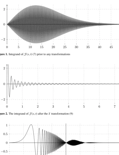
The evaluation ofJ(s,t) is extremely difficult due to the spherical Bessel function jλ(vx), particularly

when λ andvare large. The rapid oscillations of the integrand of J(s,t) (7) can be observed in Figure 1.

3.1 Application of theS transformation

TheS transformation [2], converts the integrals involving spherical Bessel functions into sine integrals by first repeatedly differentiating with respect toxfollowed by dividing byx. Using this transforma-tion,J(s,t) Eq. (7) becomes

J(s,t)= 1 vλ+1

_∞ 0    _d

xdx

λ

 xnx+λ+1

ˆ kν12

_R

21γ12(s,x)

_γ₁₂₍_s_,_x₎nγ₁₂

ˆ kν34

_R

34γ34(t,x)

_γ₃₄₍_t_,_x₎nγ₃₄

    

sin(vx) dx. (9)

Now by letting

g(s,t,x)≡g(x)=

_d

xdx

λ

 xnx+λ+1

ˆ kν12

_R

21γ12(s,x)

γ12(s,x)nγ12 ˆ kν34

_R

34γ34(t,x)

γ34(t,x)nγ34

 

, (10)

the integral in (9) can be rewritten as:

J(s,t)= 1 vλ+1

∞

0 g(x) sin(vx)dx. (11)

Since g(x) in Eq. (10) is a slowly decaying analytic function on (0,_∞) and v is constant, the semi-infinite integral after theS transformation (11) is a suitable candidate for a DE transformation.

4 DE transformation

The DE transformations (see Ooura and Mori [13, 14] for details) provide an efficient way to approx-imate integrals of the form:

I=

_∞

0 f0(x) dx =

_∞

0 g0(x) sin(vx) dx, (12)

whereg0(x) is a slowly decaying analytic function on (0,+_∞), andvis a constant. Letφ(τ) be such thatφ(τ) ∼τasτ_{→ ∞}andφ(τ) ∼0 asτ_{→ −∞}, and letM be some large positive constant. The variable transformationx=Mφ(τ) results in:

I=M

∞

−∞f0(M

φ(τ))φ(τ) dτ. (13)

The trapezoidal formula with a constant mesh sizeh:

I = Mh

∞

n=−∞

f0Mφ(nh)φ(nh) ≈ Mh N+

n=N−

(4)

In our application, this summation is not symmetric. For future reference, we define:

Sφ

n = Mh · f0Mφ(nh)φ(nh) =⇒ I ≈ N+

n=N−

Sφ

n. (15)

as well as

Iφ

N+ =

N+

n=0 Sφ

n and IφN−= −1

n=N−

Sφ

n. (16)

Two possible DE transformation functions are [13, 14]:

φ1(τ)=₁₋_exp(₋τ_K_sinh_τ₎ and φ2(τ)= ₁₋_exp(₋₂_x₋_α₍₁τ₋_e₋τ₎₋_β_(eτ₋₁₎₎, (17)

whereK=6,α=β/1+Mlog(1+M)/4π, andβ=1/4.

4.1 Application to the spherical Bessel integral

Sinceg(x) (10) is slowly decaying and analytic on (0,_∞), the integral in (11) is of the same form as the integral in (12). It follows thatJ(s,t) (11) can be approximated using the DE transformation. Applying the transformationx=Mφ(τ) to (11) results in:

J(s,t)≈_vMhλ+1 N+

n=N− g

 Mφ

nh+ θ

M

 φ

nh+ θ

M

=JM(s,t), (18)

wheregis defined in (10).

5 Numerical discussion

The approximation (18) was implemented in Python with the symbolic computation package SymPy, and calculations were completed using IEEE 754 double precision. To ensure that our integrator produced correct approximations, we compared our results with the output of a MATLAB built-in nu-merical integration function that uses global adaptive quadrature. In our implementation, we truncated the summation atN+>0 whenS

φ

N+/I φ

N+

<10−15_{and at}_N

−<0 whenSφN−/I φ

N−

<10−15_.

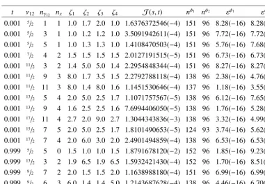
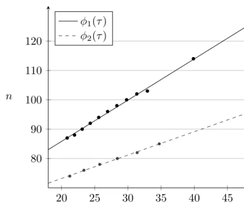
As can be seen in Figure 1 and Figure 2, theS transformation converts the spherical Bessel inte-grals into a simpler sine integral, but the integrand has slow convergence (Figure 2). The convergence is greatly improved by applying a DE variable transformationx = Mφ(τ) (Figure 3). Because the transformation induces rapid convergence to zero, sinc quadrature (trapezoidal rule) renders highly efficient approximation, and very few collocation points are required to obtain accurate results when using either transformationφ1(τ) orφ2(τ) (17). Usually, less collocation points are needed when using the transformationφ2(τ) to approximateJ(s,t) to a given degree of accuracy (Figure 4).

According to [13, 14], the relative error of the summationJM(s,t) (18) converges at a rate of approximately:

εM≈exp

−_hc, (19)

wherecis a constant.

(5)

In our application, this summation is not symmetric. For future reference, we define:

Sφ

n = Mh· f0Mφ(nh)φ(nh) =⇒ I ≈ N+

n=N−

Sφ

n. (15)

as well as

Iφ

N+ =

N+

n=0 Sφ

n and INφ− = −1

n=N−

Sφ

n. (16)

Two possible DE transformation functions are [13, 14]:

φ1(τ)=₁₋_exp(₋τ_K_sinh_τ₎ and φ2(τ)= ₁₋_exp(₋₂_x₋_α₍₁τ₋_e₋τ₎₋_β_(eτ₋₁₎₎, (17)

whereK=6,α=β/1+Mlog(1+M)/4π, andβ=1/4.

4.1 Application to the spherical Bessel integral

Sinceg(x) (10) is slowly decaying and analytic on (0,_∞), the integral in (11) is of the same form as the integral in (12). It follows thatJ(s,t) (11) can be approximated using the DE transformation. Applying the transformationx=Mφ(τ) to (11) results in:

J(s,t)≈_vMhλ+1 N+

n=N− g

 Mφ

nh+ θ

M

 φ

nh+ θ

M

=JM(s,t), (18)

wheregis defined in (10).

5 Numerical discussion

The approximation (18) was implemented in Python with the symbolic computation package SymPy, and calculations were completed using IEEE 754 double precision. To ensure that our integrator produced correct approximations, we compared our results with the output of a MATLAB built-in nu-merical integration function that uses global adaptive quadrature. In our implementation, we truncated the summation atN+>0 whenS

φ

N+/I φ

N+

<10−15_{and at}_N

−<0 whenSφN−/I φ

N−

<10−15_.

As can be seen in Figure 1 and Figure 2, theS transformation converts the spherical Bessel inte-grals into a simpler sine integral, but the integrand has slow convergence (Figure 2). The convergence is greatly improved by applying a DE variable transformation x = Mφ(τ) (Figure 3). Because the transformation induces rapid convergence to zero, sinc quadrature (trapezoidal rule) renders highly efficient approximation, and very few collocation points are required to obtain accurate results when using either transformationφ1(τ) orφ2(τ) (17). Usually, less collocation points are needed when using the transformationφ2(τ) to approximateJ(s,t) to a given degree of accuracy (Figure 4).

According to [13, 14], the relative error of the summationJM(s,t) (18) converges at a rate of approximately:

εM≈exp

−c_h, (19)

wherecis a constant.

For our calculations, we setM = 65 for the transformationφ1(τ) and M = 25 for the transfor-mationφ2(τ). These values were selected because they proved to be large enough to reach a high

0 5 10 15 20 25 30 35 40 45 50

−2 0 2

x

Figure 1.Integrand ofJ(s,t) (7) prior to any transformations

0 1 2 3 4 5 6 7

−2 0 2

x

Figure 2.The integrand ofJ(s,t) after theStransformation (9)

−1.6 ₋1.2 ₋0.8 ₋0.4 0 0.4 0.8 1.2 1.6

−1

−0.5 0 0.5 1

τ

Figure 3. The integrand ofJ(s,t) after the S and DE transformationφ1(τ) where s = 0.999, t = 0.001,

(6)

Table 1.Values ofJ(s,t) obtained using the approximation (18) with transformationsφ1(τ) andφ2(τ) (17),

wheres=0.999,ν34=ν12,nγ34 =nγ12,λ=nx,R12=2.5 andR34=5.0.

t ν12 nγ12 nx ζ1 ζ2 ζ3 ζ4 J(s,t) nφ1 nφ2 εφ1 εφ2

0.001 5_/₂ ₁ _{1 1.0 1.7 2.0 1.0 1.6376372546(}₋_{4) 151 96 8.28(}₋_{16) 8.28(}₋₁₆₎

0.001 5_/₂ ₃ _{1 1.0 1.2 1.2 1.0 3.5091942611(}₋_{4) 151 96 7.72(}₋_{16) 7.72(}₋₁₆₎

0.001 5_/₂ ₅ _{1 1.0 1.3 1.3 1.0 1.4108470503(}₋_{4) 151 96 5.76(}₋_{16) 7.68(}₋₁₆₎

0.001 7_/₂ ₄ _{2 1.5 1.5 1.5 1.5 2.0127191515(}₋_{5) 151 96 6.73(}₋_{16) 6.73(}₋₁₆₎

0.001 11_/₂ ₃ _{2 1.4 5.0 5.0 1.4 2.2954848344(}₋_{4) 151 96 8.27(}₋_{16) 8.27(}₋₁₆₎

0.001 11_/₂ ₉ _{3 8.0 1.7 3.5 1.5 2.2792788118(}₋_{4) 138 96 2.38(}₋_{16) 4.76(}₋₁₆₎

0.001 11_/₂ _{11 3 8.0 1.4 8.0 1.6 1.1451530646(}₋_{4) 137 96 1.18(}₋_{16) 3.55(}₋₁₆₎

0.001 13_/₂ ₅ _{4 2.0 5.0 2.5 1.7 1.1071757567(}₋_{5) 138 96 6.12(}₋_{16) 7.65(}₋₁₆₎

0.001 13_/₂ ₉ _{4 1.6 2.5 2.5 1.6 7.6994406050(}₋_{5) 138 96 1.76(}₋_{16) 5.28(}₋₁₆₎

0.001 17_/₂ _{11 4 2.7 2.0 9.0 2.7 1.3044343836(}₋_{3) 138 96 3.32(}₋_{16) 4.99(}₋₁₆₎

0.001 15_/₂ ₇ _{5 2.0 5.0 2.5 1.7 1.8101490653(}₋_{5) 124 93 3.74(}₋_{16) 5.62(}₋₁₆₎

0.001 17_/₂ ₇ _{4 2.0 6.0 3.0 2.0 2.4901494859(}₋_{4) 138 96 6.53(}₋_{16) 6.53(}₋₁₆₎

0.999 5_/₂ ₅ _{0 1.5 1.0 1.0 1.5 1.8791678120(}₋_{2) 152 96 1.85(}₋_{16) 9.23(}₋₁₆₎

0.999 13_/₂ ₃ _{2 1.9 6.5 1.9 6.5 1.5932421430(}₋_{4) 152 96 1.70(}₋_{16) 8.51(}₋₁₆₎

0.999 9_/₂ ₇ _{2 2.0 1.5 1.5 2.0 1.1638988180(}₋_{4) 151 96 6.99(}₋_{16) 6.99(}₋₁₆₎

0.999 9_/₂ ₆ _{3 6.0 1.4 1.4 5.0 1.2143687628(}₋_{4) 138 96 4.46(}₋_{16) 6.70(}₋₁₆₎

0.999 9_/₂ ₇ _{3 2.0 1.4 1.4 5.0 6.5370962436(}₋_{5) 138 96 4.15(}₋_{16) 6.22(}₋₁₆₎

•Numbers in parentheses represent powers of 10.

•nφ1_and_nφ2_{represent the total number of collocation points used for the summation in (18).} •The values forMused in the summation (18) areM=65 forφ1(τ) andM=25 forφ2(τ).

•εφ1_and_εφ2_{are the approximate relative errors as in (20) using transformation}_φ₁_and_φ₂_{, respectively.} •Summation is truncated atN+>0 whenSφ_N₊/Iφ_N₊<10−15and atN−<0 whenSφN−/I

φ

N−

<10−15_.

accuracy, while still small enough to keep the calculation times low. The need for a higher valueM for the transformationφ1(τ) in comparison with the lower valueM for the transformationφ2(τ) is a feature similar to the results reported in [1] for the three-center molecular integrals.

We calculate the relative approximate error of the approximation by:

εφ ₌

Sφ

N+

Iφ

N+

(20)

whereSφ

N+andI φ

(7)

Table 1.Values ofJ(s,t) obtained using the approximation (18) with transformationsφ1(τ) andφ2(τ) (17),

References

[1] J. Lovrod, H. Safouhi, Molecular Physics (2019) 12 pp., DOI:10.1030/0026867.2019.1619854
[2] H. Safouhi, J. Phys. A: Math. Gen.34, 2801–2818 (2001)
[5] I. Shavitt,The Gaussian function in calculation of statistical mechanics and quantum mechanics, Methods in Computational Physics. 2. Quantum Mechanics(edited by B. Alder, S. Fernbach, M. Rotenberg, Academic Press, New York, 1963) pp. 1–45
[6] E. Steinborn, E. Filter, Theor. Chim. Acta.38, 273–281 (1975)
[7] G.N. Watson,A Treatise on the Theory of Bessel Functions(Cambridge University Press, Second Edition, Cambridge, UK, 1944)
[8] E. Filter, E.O. Steinborn, Phys. Rev. A.18, 1–11 (1978)
[9] E.U. Condon, G.H. Shortley,The Theory of Atomic Spectra(Cambridge University Press, Cam-bridge, UK, 1951)