The design, calibration and usage of a solid scattering and absorbing phantom for near infra red spectroscopy
Michael Firbank B.Sc
Thesis submitted for the degree of Doctor of Philosophy (Ph.D) at the University of London.
Department of Medical Physics and Bioengineering. University College London.
Acknowledgements
Many thanks must go to my supervisor, Prof. David Delpy for providing such enthusiastic encouragement throughout the project, and for reading the seemingly endless number of drafts of the thesis. Also to Dr Jein Hebden for his encouragement as part of his search for the ultimate imaging phantom. José Pes created the collimators from my designs, and gave lots of advice on lathe operation. Mutsu Hiraoka improved the Monte Carlo code written by Dr Net van der Zee. Other members of the department whose collective wisdom I benefitted from include Arlene, Clare, Dave, Humberto, Mark, Martin, Matthias, Matthias, Miles, Steve, Tim and Tony.
I am grateful to Jim Cambell of Zeneca Ltd for discussions on infra-red dyes, and for the numerous samples of dyes he provided. Also to Merck for information and samples of their wondrous amorphous silica spheres. To Prof. Boyde for allowing me to use his bone saw, and to Fred Stride for letting me loose on his scanning electron microscope.
Abstract
Following a review of methods for measuring the optical properties of tissue, the majority of this thesis is concerned with the design, construction, calibration and use of a solid, tissue equivalent phantom.
The phantom material is a clear polyester plastic. This is obtained in unpolymerised form, scattering particles and absorbing dyes are added to it, and it is then polymerised to form a stable solid.
Purely scattering and absorbing phantoms were made separately, and their optical properties were measured using a specially built system. This has a co-linear collimated light source and detector, and measures the unscattered light transmitted through a
sample as a function of its thickness.
Other methods of measuring the optical coefficients of tissue were tested with this phantom. One of these uses integrating spheres to measure the transmitted and reflected light from a sample. A model of light transport (in this case a Monte Carlo model) is used to convert these measurements into scattering and absorption coefficients. It was found that the measurement of scattering coefficient was reasonably accurate, but that the absorption coefficient was overestimated at the low values typical of tissue. A measurement of the optical properties of bone was made with this system. The other system investigated uses the diffusion theory to calculate optical properties from measurements made through a thick slab.
The material was also employed to create a test phantom for near infrared spectroscopy machines. This provides a diffusing medium with an attenuation that is variable in discrete steps over three orders of magnitude. The relative attenuation between steps is totally wavelength independent. This phantom was adopted by the EC concerted action on near infrared spectroscopy and imaging.
Finally, the phantom was used to create test objects with which to investigate the
Contents
List of Figures . 10
Chapter 1
Medical imaging and monitoring techniques ...15
1.1 Introduction ...15
1.2 Alternative imaging techniques ...16
1.2.1 Radiography ...16
1.2.2 Positron emission tomography (PET) ...17
1.2.3 Ultrasound ...17
1.2.3.1 Doppler ultrasound ...18
1.2.4 Nuclear magnetic resonance (NMR) ...18
Chapter 2 Near infra red spectroscopy and imaging ...21
2.1 Introduction ...21
2.2 Near infra red spectroscopy ...21
2.3 Imaging with infra red...24
2.3.1 Simple imaging ...24
2.3.2 In line measurements ...25
2.3.3 Time gated backprojection ...25
2.3.4 General inverse technique ...26
3.1 Introduction . 28
3.2 Absorption . 28
3.2.1 Absorbing chromophores in vivo ...29
3.2.1.1 Water ...29
3.2.1.2 Lipids ...30
3.2.1.3 Haemoglobin ...31
3.2.1.4 Myoglobin ...33
3.2.1.5 Cytochromes ...33
3.3 Scattering ...34
3.3.1 Angular distribution of scattered light ...34
3.3.2 Mie theory of single scattering by spherical particles ...35
3.3.3 Rayleigh theory of light scattering ...38
3.3.4 Variation of scattering with wavelength ...38
3.3.5 Causes of scatter in vivo ...40
Chapter 4 Lightpropagation in tissue ...41
4.1 Models of light propagation in tissue ...41
4.1.1 Discrete ordinates or Kubelka Munk theory ...41
4.1.2 The radiative transfer equation ...42
4.1.2.1 Finite elements method ...44
4.1.3 Random walk model ...44
4.1.4 Monte Carlo simulations ...45
Chapter 5 Review of techniques for measuring the optical properties of tissue ...47
5.1 Introduction ...47
5.2 Single scattering phase function ...47
5.3 Scattering and absorption coefficients ...49
5.3.1 Direct measurement ...49
5.4 Review of the optical properties of tissue ...50
Chapter 6 Measurement of the optical properties of tissue and phantom materials ... . 52
6.1 Introduction ... 52
6.2 Direct measurement of absorption and scattering coefficients... 52
6.3 Phase function measurements ... 56
6.4 Simultaneous measurement of p. and using a pair of integrating spheres... 59
6.4.1 The reflectance sphere ...61
6.4.2 The transmittance sphere ...62
6.4.3 Calibration and improvements to the system ...64
6.4.4 Monte Carlo inversion ...68
6.5 Measurement of optical properties from transmission through a slab... 68
Chapter 7 Opticalproperties of skull ...70
7.1 Measurement of the optical properties of skull ...70
7.1.1 Sample Preparation ...70
7.1.2 Measurements ...71
7.1.2.1 Results ...71
Chapter 8 Phantoms...74
8.1 Introduction ...74
8.2 Choice of phantom for this work ...75
8.3 Components of the phantom and production thereof ...76
8 .3.1 Index matching liquid ...77
8.4.1 Scattering properties . 78
8.4.2 Angular scattering function ...82
8.4.3 Absorption properties ...84
8.4.4 Refractive index of the phantom ...86
8.4.5 Stability of the phantoms ...87
8.4.6 Scattering suspensions of silica spheres ...88
8.4.6.1 Scattering properties of the silica spheres ...89
8.4.6.2 Angular scattering function ...91
Chapter 9 Phantom application for spectroscopy and imaging ...93
9.1 Introduction ...93
9.2 Comparison of methods for measuring optical properties ...93
9.3 Integrating spheres ...94
9.3.1 Absorption coefficient ...94
9.3.2 Scattering coefficient ...96
9.4 Diffusion theory fit ...99
9.5 Spectroscopy phantom ...100
9.5.1 Design of the phantom ...100
9.5.2 Modus operandi ...101
9.5.3 Measurements and results ...102
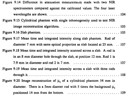
9.6 Phantoms for imaging ...105
9.6.1 The effect of coupling liquid ...106
9.6.2 Preliminary imaging experiment ...108
Chapter 10 Discussionand further work ...110
10.1 Phantom material ...110
10.2 Spectroscopy phantom ...111
10.3 Imaging phantoms ...112
Conclusions
. 115
List of Figures
Figure 2.1 Light intensity vs time measured from a ultrashort pulse at time zero,
showing the mean time of flight. Data generated using the diffusion
equation...23
Figure 2.2 Input and output light distributions for an intensity modulated phase
system...23
Figure 2.3 Absorption coefficient of water in range 650 to 1025 nm...24 Figure2.4 In line measurements ... 25
Figure 3.1 The absorption coefficient of water in the range 0.2 - 2.6 Lm.
...30
Figure 3.2 The absorption spectra of pork fat in the range 800-1100 nm.
...31
Figure 3.3 The absorption spectra of Haemoglobin in both oxygenated and
deoxygenated states in the range 450 to 1000 nm...32
Figure 3.4 The absorption spectra of several haem compounds in the near infra
redbetween 650 and 1000 nm...32 Figure 3.5 The absorption spectra of the cytochrome enzymes in the range
500-l000nm...33
Figure 3.6 Showing the variation of scattered light intensity with particle size. .. 37
Figure 3.7 Showing the variation of scattering cross section and g factor with
wavelength for a particle of diameter 1pm...39
Figure 6.1 Showing the system for measuring collimated transmission through
asample...53
Figure 6.2 Showing a cross-section of one of the collimators...53
Figure 6.3 Showing the extrapolated variation of refractive index with
wavelength for water and polystyrene. Symbols are literature values, solid
lineextrapolation... 55
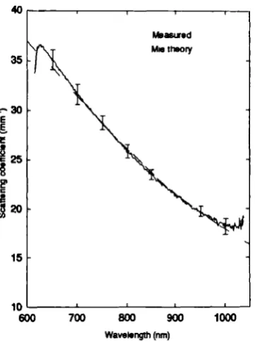
Figure 6.4 Showing the measured scattering coefficient of polystyrene spheres
as compared with the value calculated by Mie theory. Errors bars ± 1
Figure 6.5 Showing the goniometer setup for measurements from 0 - 90° . 57
Figure 6.6 Goniometer setup for measuring angles between 900 and 170° ... . 57
Figure 6.7 System response of the goniometer system ...58
Figure 6.8 Showing the effect of stopping specularly back reflected light form
beingdetected...58
Figure 6.9 Integrating sphere arrangement for measuring diffuse reflectance and
transmittance...60
Figure 6.10 Showing a detail of the integrating sphere with the sample...60
Figure 6.11 Showing the original collimation system for the integrating
spheres...65
Figure 6.12 Showing the improved collimator for the integrating spheres...65
Figure 6.13 Graph showing the reflectance from the standards as measured using
the integrating spheres in comparison with the manufactures data...66
Figure 6.14 Showing the difference between the measured and expected
reflectance from polished silver and clear polyester samples...67
Figure 6.15 Showing the experimental configuration for measuring the temporal
distributionof light ...69
Figure 7.1 The phase function of bone at 800nin. Error bars ± 1 sd ...71
Figure 7.2 Transport scattering coefficient and g value of bone. Error bars ± 1
sd...72
Figure 7.3 Scattering and absorption coefficients of bone. Error bars ± 1 sd. The
spectrum corrected for a systematic error of + 0.0 15 mm is also
shown(dotted line) ...72
Figure 8.1 The effect of different catalysts on the absorption spectra of a dye
(PRO JET 900 NP, Zeneca Ltd)...76
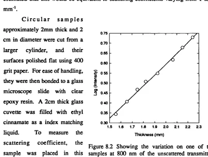
Figure 8.2 Showing the variation of unscattered transmitted light against
thickness on one of the samples at 800 nm...78
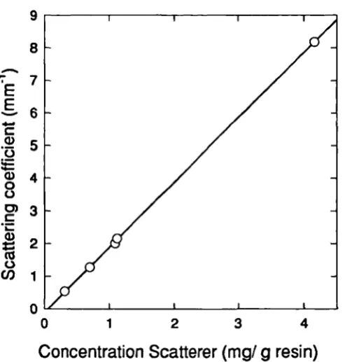
Figure 8.3 The variation of scattering coefficient with scatterer concentration at
800 nm for five samples of the phantom material...79
Figure 8.4 Scattering coefficient versus wavelength for 5 different samples,
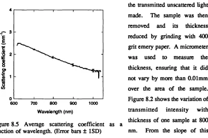
normalised for scatterer concentration...79
Figure 85 Average scattering coefficient as a function of wavelength. (Error bars
Figure 8.6 Particle size distribution as measured with an electron microscope. (2
samplesand total of 300 particles) ...81 Figure 8.7 Comparison between the measured scattenng coefficient and the
theoretical value (calculated using the measured size distribution)...81
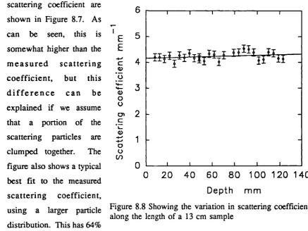
Figure 8.8 Showing the variation in scattering coefficient along the length of a
13 cm sample ...82
Figure 8.9 Averaged phase function (from 3 samples) of titanium dioxide
particles in polyester resin at 800 nm (± 1SD) ...83
Figure 8.10 Showing the variation of g with wavelength (± 1 SD). The
systematic error is ±0.03. Also shown is the value calculated from Mie
theory using the measured size distribution and the distribution from the
bestfit to .L...83 Figure 8.11 Absorption spectra of some dyes. S 103508/5 (solid line) PRO JET
900NP (dashed line) and S159521/1 (dotted line)...84
Figure 8.12 The absorption spectra of the resin (± 1 SD) ...84
Figure 8.13 Graph showing the variation of absorption coefficient with
wavelength for several different samples of dye in resin...85
Figure 8.14 Graph showing the average absorption spectrum for dye in resin in
comparison with the absorption coefficient for the dye in liquid
styrene...85
Figure 8.15 Showing the measured time delay of an ultra short pulse of light
through a 17 cm thick clear block of polyester (at 800nm)...86
Figure 8.16 Showing the measured variation of refractive index with wavelength.
The refractive index of polystyrene shown for comparison...87
Figure 8.17 Showing the variation of absorption coefficient with time. Upper set
of data at 720 from S 103508/5. The other two are from PRO JET 900
NP. Triangles show data from samples kept in the dark ...88
Figure 8.18 The scattering coefficient of the silica spheres in styrene: smooth
data calculated, noisy data measured values...89
Figure 8.19 The measured scattering coefficient of the spheres suspended in
solid resin. Also the scattering coefficient calculated using the empirical
refractive index and that of polystyrene...90
Symbol: measured points. Solid line: theory . 91
Figure 8.21 Anisotropy factor g as determined from the measured phase
function. Solid line is theoretical value...92
Figure 9.1 Comparison of L,, measured using integrating spheres and by the collimated system measurements. A total of 13 samples used. The
regression line has an intercept of 0.014 and a slope of 0.97 ... . 95
Figure 9.2 Wavelength variation of the ta• The upper curve shows the average of 3 samples measured by the integrating spheres. The lower data is
t measured with the collimated system... 95
Figure 9.3 Difference between the integrating sphere .t1 and collimated system
. Dotted line is the average difference...96
Figure 9.4 p, of Ti02 suspension measured on 15 samples with integrating
spheres compared with that calculated from collimated system data. The
regression line shown has a slope of 0.87 and an intercept of 0.47 ...97
Figure 9.5 p of silica sphere suspensions measured on 7 samples with the integrating spheres plotted against the calculated values. The regression
line has a slope of 0.9 and an intercept of 0.32 mm4...97
Figure 9.6 Scattering coefficient vs wavelength for Ti02 particles from
integrating sphere data (lower curve) and collimated system...98
Figure 9.7 Scattering coefficient vs. wavelength for integrating sphere data
(lower curve) and collimated system for silica particles ...98
Figure 9.8 Scattering coefficient as measured using the diffusion approximation
fit to the TPSF vs collimated measurements. The solid line is the unity
line, not a regression...99
Figure 9.9 Absorption coefficient as measured using diffusion approximation fit
to the TPSF. Unity line shown...99
Figure 9.10 Phantom for use in calibrating spectroscov instruments...101
Figure 9.11 Showing cut out view of slider hole and holder...101
Figure 9.12 Variation of attenuation with wavelength for the calibration phantom
8 mm hole, plus the attenuation difference between 6 and 8 mm holes. .. 103
Figure 9.13 Showing the variation of attenuation with hole diameter for the
spectroscopy phantom. Solid line is the caluculated values from equation
Figure 9.14 Difference in attenuation measurements made with two NIR spectrometers compared against the calibrated values. The four laser
wavelengthsare shown...104 Figure 9.15 Cylindrical phantom with single inhomogeneity used to test NIR
imagereconstruction algorithms... 105 Figure9.16 Slab phantom... 105 Figure 9.17 Mean time and integrated intensity along slab phantom. Rod of
diameter 7 mm with same optical properties as slab located at 25 mm. .. 107 Figure 9.18 Mean time and integrated intensity scanned across a slab. A rod is
in an 8 mm diameter hole through the slab, at position 12 mm. Rod 1 is
7.9 mm in diameter and rod 2 is 7 mm...107 Figure 9.19 Mean time and integrated intensity across a slab with three rods
throughit...108 Figure 9.20 Image reconstruction of .ta of a cylindrical phantom 54 mm in
diameter. There is a 5mm diamter rod with 5 times the background p
Chapter
Medical imaging and monitoring techniques
1.1 Introduction
The work described in this thesis is based around the development, testing and
usage of a material which matches the optical properties of tissue in the near infra red
region. The material (or phantom) is designed to be an aid to investigators in near infra
red spectroscopy and imaging.
Near infra red spectroscopy (NIRS) was first used by Jöbsis in 19771* can be
used in vivo to measure the relative quantities of infra red absorbing substances, such
as oxygenated and deoxygenated haemoglobin, and oxidised and reduced cytochrome
aa3, the terminal enzyme in the respiratory redox chain. Measurement of the amount of
water in the tissues is also possible using derivative spectroscopy. Imaging systems
which use infrared light are now also being developed, which as well as determining the
absorption distribution, may also provide some information about the local optical
scattering properties. This will make it possible to distinguish between different tissue
types. MRS imaging systems are likely to be used in the study of oxygen availability
in the neonatal brain, particularly the localisation of ischaemic regions, and the detection
of tumours, especially in the female breast. Tumours often have a greater absorption,
due to their enhanced vascularityth. They also have different light scattering properties
to the surrounding tissue, resulting from their different structure.
The advantage of the NIRS technique is that it is non invasive, and that there is
no evidence of it causing damage. It can therefore be used continuously. This is very helpful clinically, where periodic or continuous monitoring can be used to observe the
monitoring, several well established non optical imaging techniques will be discussed, with respect to their clinical use and their advantages and disadvantages.
The next four chapters describe the optical properties of tissue in the near infra red, the modelling of light propagation in tissue and the specific techniques of NTR spectroscopy and imaging. This hopefully will give an understanding of the problems associated with the technique, and of the areas in which a stable tissue equivalent material is needed for investigation.
1.2 Alternative imaging techniques
1.2.1 Padiociraphy
X rays are not greatly scattered by soft tissues, and the different tissue types absorb differing fractions of the incident radiation, ranging from fat which absorbs very little, to bone which is the strongest absorber. In simple radiographs, the source is placed on one side of the area in question, and a photographic plate detector on the other side. This method produces the familiar X ray pictures of bones. When it is used for breast tumour detection, this technique is called mammography; tumours often absorb more strongly than the surrounding tissue, since they are more dense, and as micro calcifications are present in 40% of tumours 2. Using mammography, 93% of tumours are detected3.
1.2.2 Posftron emission tomoraphy (PET)
This technique involves the use of an injected radioactive isotope which decays, producing a positron. The positron annihilates almost immediately on meeting an electron in the surrounding medium, producing two photons (511 KeV) which have equal momentum and hence travel in opposite directions. Because of their high energy, there is little interaction between these photons and the surrounding tissue. The two photons are then detected using a ring of detectors (scintillator crystal and photo multiplier tubes) linked to coincidence counters7. The fact that the two photons arrive almost simultaneously on either side of the object allows spurious signals to be ignored and improves signal localization. The isotopes used in PET include 'SO, 11C, '3N and
'8F. These isotopes are used to label certain compounds, eg H2'50 and from the detected photons, an image of the compound distribution can be built up. PET has been used to measure cerebral blood flow using H 2'50, cerebral blood volume using inhaled C'50, which binds strongly to haemoglobin, and glucose metabolism using ' 8F labelled deoxy-glucose. The isotopes used all have a relatively short half life (123s for 'O up to 110 mins for '8F). The disadvantages of the method are that it uses radioisotopes invasively and that due to their short half life, the isotope preparation is expensive, and must be performed nearby in a large cyclotron. The detection equipment is also bulky and cannot be used at the bedside, which is an important consideration when attempting to study preterm infants or patients requiring intensive care.
1.2.3 Ultrasound
the reflections from near the surface do not swamp those from deeper inside. Ultrasound can only be used to image the arrangement of different types of tissue, as it does not provide functional information.
1.2.3.1 Doppler ultrasound
Blood velocity can be measured with ultrasound by utilising the doppler effect. This effect causes the frequency F0 of a reflected wave to shift by an amount dF, proportional to the velocity, v of the reflector relative to the detector, given by
dF - 2F0
.cos(a)
(1.1)
C
where a is the angle between the direction of movement and the detector and c is the velocity of the waves in the medium.
To get an average blood velocity distribution for all moving particles in the sound beam, a continuous source is used. To determine the velocity at one particular depth, a pulsed source is used, the depth being determined by the phase difference between input and detection. Blood flow can only be calculated using this method if the volume of the blood vessels, and the angle of the vessel to the ultrasound detector, are known, and remain constant throughout the measurement.
Both ultrasound and doppler ultrasound are non invasive, safe and can be used at the bedside.
1.2.4 Nuclear mainetic resonance (NMR)
co-yB
where q (1.2)
- 2itm
q and m being the charge and mass of the proton respectively.
If an electromagnetic pulse of the same frequency as the Larmor frequency is applied to the nuclei, with its magnetic field component perpendicular to B there will be a strong interaction or resonance. This causes the orientation of the nuclei with respect to B to change by an amount which depends on the strength and duration of the pulse. Once the pulse has finished, the nuclei which continue rotating around the applied magnetic field now produce a small magnetic field component transverse to B. This rotating transverse field induces a current in a coil surrounding the sample, which is the signal detected by NMR. The time taken for the nuclei to return to their thermal equilibrium along B is known as T1 . Due to small scale inhomogeneities, individual nuclei have slightly different rotational frequencies; this results in their magnetic fields rotating relative to each other, and hence a reduction in the overall directional signaL The time for this to occur is known as T 2. The time constant of the decay of the induced signal in the coil, a combination of T 1 and T2, is known as T2*. The nucleus most commonly used for imaging in tissue is that of hydrogen in water.
Several parameters can be measured in NMR, including T 1, T2, T2 , nuclei density, and change in co with chemical environment. In order to produce a 2D image of an object, additional magnetic fields are applied, which vary linearly along the axis, so that the applied rf pulse only interacts with the nuclei with the appropriate Larnior frequency, ie only those in a defined position along the axis. Different types of tissue can be distinguished using NMR, depending on their T 1 and T2, which in turn depend on their molecular environment. Excellent structural images can be produced for soft tissues.
Chapter 2
Near infra red spectroscopy and imaging
2.1 IntroductIon
In this chapter, the use of near infra red spectroscopy to measure the relative oxygenation state of the blood will be described. Problems associated with the technique will be discussed, along with methods used to circumvent them.
The potential use of infra red light to produce images of human tissue is described in the last part of the chapter.
2.2 Near Infra red spectroscopy
If a non scattering medium is illuminated with a collimated beam of light, the transmitted intensity, I is dependant upon the specific absorption coefficient a, the concentration of the absorber,C and the thickness f of the medium. The exact
relationship is given by the Beer Lambert law:
I - l0 exp(-uCI) (2.1)
where I,, is the incident intensity. Obviously, if the distance travelled through the medium and the specific absorption coefficient of the absorber are known, its concentration can be calculated.
absorption spectra of the absorbing compounds.
Using the technique for measuring across human tissue, a problem is caused by
the high degree of light scattering. This has the effect that the light takes a convoluted
path, and so the distance travelled is much longer than the distance between its entrance
and exit points on the tissue surface.
In such a case, the pathlength is not only unknown, but does not have a singular
value. It varies nonlinearly with source-detector distance and geometry, and is also
dependent upon the absorption coefficient 10. It is however, still possible to quantify
changes in absorber concentration if we know, or can measure the relationship between the average photon pathlength, L and the source/detector distance,I and assume that the
absorption coefficient does not vary too much. The Beer Lambert law can be modified
in such circumstances" to take scattering into account to give:
I - I0e<+K (2.2)
where the differential pathlength factor, = LIQ, and K is a geometry and tissue
dependant constant.
If only intensity changes are measured from some arbitrary starting point,
assuming that K stays constant, this can be rewritten
EtI - (2.3)
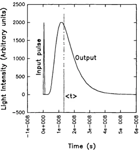
By measuring the average time <t> for an ultrashort pulse of light to cross the medium, (see Figure 2.1) the effective or average path length, L, can be determined' 3 using
L = c<t>, c being the speed of light in the medium. This path length can be measured
as a function of optode spacing, and an average conversion factor I determined.
Another method of measuring L is to use intensity modulated light, and to
measure the phase angle $ between the transmitted and the detected modulated light (see
Figure 2.2). Provided that the modulation frequency, f is less than 200 MHz, $ relates
to the average pathlength by'475
L (2.4)
2iq'
where $ is the phase difference. Using frequency modulation is equivalent to using the
2500 I I
a)
2000
1500 0
cx 0 U1 c aD aD
o 0 0 0 0 0 0 0 o o o o a a a a
I + I I I I
4) 4) 4) 4) 4) 4) 4) 4)
0 C P) It)
Time (s)
Figure 2.1 Light intensity vs time measured from a ultrashort pulse at time zero, showing the mean time of flight. Data generated using the diffusion equation.
sample
/
I
I
phase shift
T 0.04
E E
0.03
.2 0.02
4-, 0.
I-0 0, . 0.01
0.00 0.05
700 800 900 1000
Wavelength nm
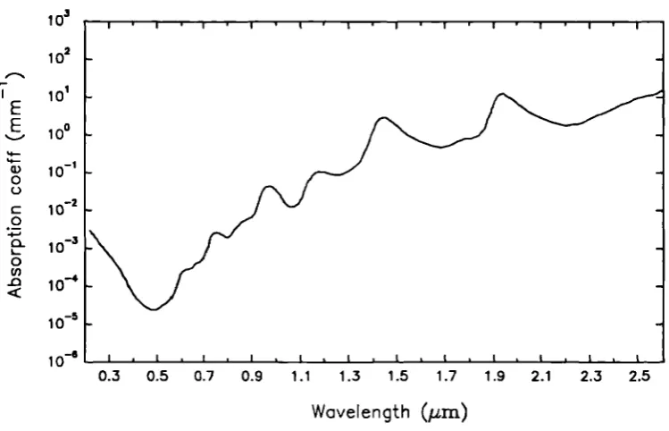
Figure 2.3 Absorption coefficient of water in range 650 to 1025 nm.
about its mean, for higher frequencies, the phase deviates from this relationship. This technique has the advantage that the equipment used to measure the pathlength is much less bulky than an ultrashort pulse laser system. This technique has been used by Sevick et al'5, Lakowicz et a116 and Duncan et al'7
Work is also being carried out into the determination of the path length using the absorption of light by water in the tissue' 8. The
concentration of water in the body is known fairly accurately, and water has some absorption bands in the near infra red region (see Figure 2.3). If, therefore, the light attenuation through tissue at these wavelengths is measured, and compared with the expected absorption, the actual pathlength travelled by the light through the tissue can be calculated via Eqn (2.2), providing that the concentration of water is known.
Tissue spectrometers using a range of these techniques have been designed to determine relative changes in tissue oxygenation, using previously measured spectra for pure oxygenated and deoxygenated haemoglobin and cytochrome aa3.49"920'
2.3 Imaging with Infra red.
2.3.1 SimrIe imacinc
Scattering medium
Sourcc
inadequate when compared to mammography, especially for small and deep lesions. In order to improve the technique, it is necessary to reduce the amount of scattered light detected, or to use some knowledge of aight transport in tissue to try to correct for the blurring effects of scattering.
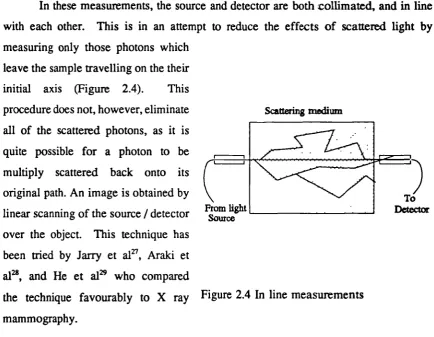
2.32 In line measurements
In these measurements, the source and detector are both collimated, and in line with each other. This is in an attempt to reduce the effects of scattered light by measuring only those photons which
leave the sample travelling on the their initial axis (Figure 2.4). This procedure does not, however, eliminate all of the scattered photons, as it is quite possible for a photon to be multiply scattered back onto its original path. An image is obtained by linear scanning of the source / detector over the object. This technique has been tried by Jarry et alp, Araki et af, and He et al who compared the technique favourably to X ray mammography.
Figure 2.4 In line measurements
2.33 Time cated backiroiection
straight through path, and derived an expression for the resolution, Ax as a function of the time gating At:
(cAt+d) v
' i -t 2/(cAt+d)2 r- ____mu
2
(23)
Ax l/2rmu
where c is the speed of light in the medium, and d the thickness of the medium. This expression is only valid when rmu is less than the width of the medium, for larger values, it tends to overestimate the resolution
This process is identical to that used in X ray tomography 3' and has been used by several investigators3Z33.i5.i6.37. The advantage of this technique is its simple concept, but it has the obvious disadvantage that the measured light intensity is much reduced and falls exponentially with sample thickness, thus reducing the signal to noise ratio.
A development of the technique has been used by Hebden 38 who measured the whole temporal distribution of light (over -2000 ps), and fitted the data to a temporal distribution calculate using the diffusion equation. The diffusion equation fit was then used to predict the integrated intensity c er the first few picoseconds. Improved resolution is obtained with this method.
2.3 4 General inverse technaue
This is a general mathematical technique for comparing the measured intensity with a mathematical model. For any given geometry and source, we can define a forwaixi operator, F, which gives some measurable quantity as a function of the positionally varying optical properties of the medium, 'a and given by
F(.t) - J. (2.6)
A(s) - F(p^)-F(j.t) . (2.7)
In order to determine the optical image, t from the measurements, the Moore Penrose
inverse can be used iteratively,39
(k.1) - [(A 'A)'A ][J - F(.L(k))] (k) (2.8)
where k indicates the iteration number, and * indicates an adjoint operator, ie F*F = p..
Only the first iteration can be obtained using exact solutions of the diffusion equation, as this is only soluble for the homogeneous case. However, some more flexible model such as the finite elements of the diffusion equation, or the random walk model85' could be used to give further iterations. The quantities which can be measured and used as data for this method of reconstruction include the integrated intensity as a function of position,I()
(2.9)
<t>, the mean of the temporal distribution (see (1.31))
ftI,t)dt
-
_________ , (2.10),E,t)dt
or, if amplitude modulated light is used, the phase shift and modulation depth, M (see Figure 2.2)
(I / d)jztec:ed (2.11)
M- _______
Chapter 3
Absorption and scattering of light
3.1 Introduction
In this chapter, the theory of light absorption will be discussed, together with the causes of light absorption in tissue. Models of light scattering will then be presented, along with a brief discussion of the causes of light scattering in tissue.
3.2 Absorption
Bouger404' in 1729 derived the first relationship between the thickness of a
material and its absorption of light. Lambert42 later expressed Bouger's relationship mathematically. The Lambert-Bouger law, as it is often known, states that for a pure absorber, a layer of thickness dD absorbs a fraction dill of the incident light intensity I, ie that di/l = I.Lad where .La is a constant for the material, called the absorption coefficient.
The collimated light I measured when a collimated light beam of intensity l passes through t mm of non scattering material is therefore
/ - '0 1•t (3.1)
-4iw t 1-I0exp
A
J
(3.2)
Beer43 in 1852 derived a similar relationship for absorption in terms of the concentration of absorbing molecules in a medium. This states that the absorption coefficient is proportional to the concentration of the absorber. Combining the two laws, we obtain the so called Beer-Lambert law, which states that
I - J0 e° (3.3)
where C is the concentration of the absorber and a the absorption coefficient per unit concentration Ic the specific absorption coefficient, usually quoted in units of mm' mmol'. This equation can be rearranged as
1og10(e).aCQ C1 A - i "I (3.4)
where A is the absorbance or the optical density, and s is the base 10 absorption coefficient, often called the specific extinction coefficient, and usually quoted in units of cm' mmol'. In this thesis, base e coefficients will be used in general, although both are widely used in the literature. For a solution containing a mixture of absorbing substances, the absorption coefficients sum, so the optical density is simply given by
A - (e 1C1 +e2C2^...+çC,)v . (3.5)
3.2.1 AbsorbIng chromophores in viva
3.2.1.1 Water
E E
9-a) 0 C.)
0 ci
0 Cl, .0
102 101 100 10_I 1 0_2
1 1 1 0
0.3 0.5 0.7 0.9 1.1 1.3 1.5 1.7 1.9 2.1 2.3 2.5 Wavelength (nm)
Figure 3.1 The absorption coefficient of water in the range 0.2 - 2.6 jim.
to 2 j.im. As can be seen, at wavelengths longer than 1.3 jim the absorption coefficient is greater than 0.1 mm'. Such a high level of absorption makes light detection through more than one or two centimetres of tissue very difficult, limiting transmission measurements to shorter wavelengths.
3.2.1.2 Lipids
Little data is available on the absorption spectra of human lipids, but the extinction coefficient of pork fat has been measured by Conway et al and the spectrum is shown below. As can be seen, it is similar in many ways to that of water. In the adult brain, the grey matter contains 8% of lipid by mass, and white matter
17%. Lipids will therefore not contribute significantly to the overall extinction in the 600-900 nm region where the intrinsic absorption is low.
The percentage of lipid in adipose tissue, of which the breast is largely composed, is approximately 75%, which means that there, the lipid absorption must be taken into account.
0.06 E 0.05
9- 'l-a)
0.03
I:
0.00
800 850 900 950 1000 1050
Wavelength (nm)
Figure 3.2 The absorption spectra of pork fat in the range 800-1100 nm.
adults, although certain clinical diseases can lead to muscle wastage and fat deposition (eg muscular dystrophy).
There is also a contribution to all measurements of light transmission from absorption by subcutaneous adipose tissue, which will vary from individual to individual, but will tend to be larger in women.
3.2.1.3 Haemoglobin
Haemoglobin is found in the red blood cells and is The major oxygen carrying compound in the blood. There are several different forms of haemoglobin which can be found naturally in the blood, the most common are oxygenated and deoxygenated haemoglobin (Hb02 and Hb). Also found are carboxyhaemoglobin (HbCO), typically present at 2-4%, but up to 10% in smokers 48, haemiglobin (Hi), typically 0.5 - 2.5%,
1.6 E ' 1.2
0 U
0
0.
EL
.40.0
650 700 750 800 850 Wove ength (nm)
900 950 1000
approximately 84tM49, it is apparent that light absorption by haemoglobin will limit the wavelength of light used for spectroscopy across several centimetres of tissue to wavelengths above 600 nm.
T 16 E E 14
12
F° c 8 0
0 E 2
0
a-(I)
500 600 700 800 900 1000
Wavelength (nm)
Figure 3.3 The absorption spectra of Haemoglobin in both oxygenated and deoxygenated states in the range 450 to 1000 nm.
2.0
3.2.1.4 Myoglobin
Muscle contains the chromophore myoglobin. Its NIR absorption spectra is almost identical to that of haemoglobin 5° although the spectra are different in the UV and visible region. The binding of oxygen to myoglobin occurs at lower partial pressures than haemoglobin (P 1 kPa cf P 3.5 kPa for Hb). This means that in general, in well perfused tissues, most of the myoglobin is fully oxygenated.
3.2.1.5 Cytochromes
The cytochrome chain of enzymes are responsible for electron transport in the mitochondria where oxygen is reduced to form water, and ADP phosphorylated to form ATP. Cytochrome aa is the terminal enzyme in the chain, and has the strongest absorption coefficient. The absorption spectra of the cytochrome enzymes 49 are given in Figure 3.5
12 E E
L.
0
U)
-a
0 U 4-U
a)
0 (1)
500 550 600
Wave ength (nm)
0.6
0.4 r'-.._ '.
Cyt aa3 (oxi) Cyt aa3 (red) Cyt b (oxi) Cyt b (red) Cyt c (oxi) Cyt c (red)
0.2
I-0.0 t. -1--.---,--
-'...4.--.---700 800 900 1000
Wave ength (nm)
3.3 Scattering
Tissue scatters near infra red light elastically, which means that the wavelength of the light remains constant. The scattering of light is dependent on two quantities: the relative refractive index of the scatterer and its surrounding medium, and the dimensions of the scattering particle relative to the wavelength of the light. The percentage of scattered light and its angular distribution depends greatly upon the ratio of particle size to wavelength. The size of the scatterers in tissue cover the range from somewhat larger to smaller than the wavelength of near infra red light.
The scattering coefficient of a substance, is defined in much the same way as the absorption coefficient, ie
- (3.6)
where 1. is the unscattered light intensity at depth Q.
Two other parameters which can be defined are the scattering and extinction cross-sections, a and a, respectively.
w
w
a - --_ . a,--_. (3.7)
I j0 '0
where I is the total intensity incident on the particle, W the rate of energy absorption by the particle, and W the rate of energy scattering by the particle. The scattering coefficient is related to a, by
a,
(3.8) d3
where d is the average distance between particles.
3.3.1 AnQular disfribuflon of scattered Iiaht
g f(0)cosOsinO Ef(0) sinO
(3.9)
which is used in diffusion theory as a measure of the anisotropy of the scattering (see
chapter 4.1.2). g varies from 1 (totally forward scattered ight) to 0 (isotropically scattered light.
The transport scattering coefficient is defined as .t' = p(1-g). 1I(1-g) is the number of scattering events which occur before the directionality of the scattering becomes randomised. This means that in the far field, the light distribution in a scattering medium with an anisotropy factor of g and a scattering coefficient of p is equivalent to that in an isotropic scattering medium with a scattering coefficient of p( 1-g).
The Henyey Greenstein function51'52 is often used to approximate the angular dependence of scatter, f as a function of the cosine of scatter, u. It involves only the parameter g, and the ratio of reflected to incident light, or albedo, w:
f(u) - o0(1-g 2 )(1+g 2 -2gu) 3'2 (3.10)
This function gives a reasonably good approximation to the exact predictions of Mie theory (see next section), and has the advantage of being an easy expression to handle mathematically.
3.3.2 Mie theory of sinQ e scaffering by sr)herlcal iartictes
The exact theory of the scattering of light by a solid sphere was developed by Gustav Mie in l9O8. He calculated the internal and external scattered electromagnetic fields as a function of the size parameter, x and the relative refractive index, m:
2itna n
m-_! (3.11)
n
travelling in the x direction,
E - E e (3.12)
0 I
the electric and magnetic fields of the scattered wave are given by
- E(i(2,1N, -b1M,,)
H - ER(ibflN,+aRMS,fl)
(3.13)
n-i
where
M, - cos ;(cosO)h,"(kr)l0 - sin4 t1(cosO)h,'(kr)ê, M - -sin4 ir(cosO)h'(kr)i0 - cos4 t1(cosO)h,'(kr)ê,
h °(kr) N00 - sinn(n+1)sinOir(cosO)_"
+
si$t(cosO)_''')j'
{1crh,'(kr)J'
i0+cosit1(cosO) (3.14)
kr h '(kr)
NCR - cos4n(n^1)sinOit(cosO)_"_ê kr
+ cos4rc(cosO) -si$i(cosO){kTh"(kr)r
kr J,•
(e and o designate even and odd)
a - pm 2j(mx) [xj(x)]' -p 1j(x) [mxj(nu)}'
pm 2j,1(mx) [xh,°(x)]' -p 1h,'(x)
jim1"
(3
15) b-0p1j1(mx)[xh,"(x)]' -ph,°(x)[mxf0(,nx)]'
E - iE a (2n^1) °n(n+1)
it - a ____ (3.16)
sinO dl': ta
-o
and are the planar and azimuthal spherical polar angles, p and Pi are thepermeability of the medium and sphere respectively, h5(D is a spherical Bessel function
of the third kind, j a spherical Bessel function, and P' a Legendre Polynomial.
From these equations can be calculated the rate of energy scatter, W1
w -
!Re ( f(EJOHJ -
E4H,)r 2 sinOdOd (3.17)2-and using equation (3.7), a can be calculated.
a, - .?±E(2n^l)Re[a,, + b,) (3.18)
k
Not surprisingly, solutions to these equations are normally calculated numerically
using a computer, although the
equations used for this are slightly
modified for ease of calculation and 1.2 . •
convergence, the speed of convergence 1.0 ,, \
being faster the smaller the particle. o.8 \ / / From the scattered fields can be 0.8 \\
/
/\/ :
calculated the scattering and extinction 0.4 1
cross sections and the angular 0.2
dependence of scatter. The angular 0.0
scatter function Jor particles of size 0.2 , , ,
greater or equal to the wavelength is 7 7 I
Angle
highly forward weighted. Figure 3.6
- radius 10 times wavelength shows the angular distribution of radius equal wavelength
radius 1/10 wavelength
scattered light for particles which are
V2
Jcc__
r2A
(3.19)
incident light wavelength (zero represents the forward direction).
Mie theory has also been applied to other simple geometries, including elliptical
particles and hollow spheres, but is not strictly valid for particles of arbitrary geometry.
It is, however, the only accurate theory which applies to particles of size comparable
with the wavelength. A full derivation of the Mie equations for a spherical particle and
a FORTRAN algorithm to evaluate them is given in Bohren and HuffmanM.
When the particle size is less than 1/4 of the wavelength the theory simplifies,
and Rayleigh scattering theory applies.
3.3.3 Ra
yleich
theoryof IiQht
scatter nçRayleigh's theory concerns the scattering of light by particles much smaller than
the wavelength. He derived it by considering the dimensions of the variables involved,
these being the volume V of the particle, the chstance r at which observations are made,
and the wavelength of the light. His equation states that the scattered intensity, I, is given by
A similar equation can be derived from Mie theory by taking the first few terms
of the Bessel series expansion. For unpolarized incident light I, the scattered light I at
angle 0 is
I
Sit4 n a 6 m 2 -1 (3.20)
- A.4r 2 m2^2J
(1^cos2O) I
The angular dependence of scatter is thus a smusoidally varying function, and as the
radius of the particle, a, tends to zero, the distribution becomes isotropic.
3.3.4 Variation of scatterinQ with wavelength
is the changing ratio of particle size to the wavelength of the light. The
scattering cross section is highly 4 r
dependant on this ratio, especially
when the particle is approximately the 2
U)
same size as the wavelength. For " 2
U)
2
C.)
particles much smaller than the wavelength of the light, the cross
C.)
C')
section is inversely proportional to the 0
fourth power of the wavelength. This ___________________________
10 2 101 10° 10'
was shown in the section on Rayleigh wavelength (p.m)
scattering, and incidentally, is _________________________ 12
responsible for the blueness of the sky
10 and redness of sunsets" 6. For
2 08
particles much larger than the
wavelength, the scattering Cross-section 06 is approximately constant (See 04 Figure 3.7). The anisotropy of the
02 scattering also changes with
cot I I
wavelength, becoming more forward 102 10' 10° 10' biased as the wavelength gets shorter. Wavelength (tim)
The refractive index of the Figure 3.7 Showing the variation of scattering cross section and g factor with wavelength for scattering particles and medium will a particle of diameter 1.tm.
also vary with wavelength, and this is
the other cause of variation in the scattering cross section. The refractive index slowly decreases with wavelength for transparent materials, and this decrease can be approximated by using an approximation discovered by Cauchy55
BC
n =A+—^—+... (3.21)
x2
3.3.5 Causes of scoffer in vivo
Chapter 4
Light propagation in tissue
4] Models of light propagation in tissue
In order to use light therapeutically or diagnostically, it is imperative to know how it propagates through tissue, so that the degree of illumination as a function of position is known. Several methods of doing this have been developed, with varying degrees of complexity, the more important of which are described in this chapter.
Theories of light propagation through tissue usually involve treating the light as being particulate, rather than wavelike in nature. Twersky developed a theory of light transport using EM theory, but this approach is little used, being both complex and difficult to apply to anything other than simple homogeneous geometries. In addition, due to the random nature of tissue, wave effects and interference rapidly average out and become negligible.
4.1.1 Discrete ordinates or Kubelka Munk theory
The discrete ordinates method involves transforming the continuous direction variable , into N discrete values, so that
I
dci.i (r,fl) -+V" w I (r) (4.1)J4 L..dn1 R fl
Kubelka Munk theory is basically a two flux model, having a forward and backward diffuse flux in a infinite slab. It assumes isotropic irradiance and zero reflection at the boundaries of the sample 578. Using this theory, the 'Kubelka Munk' scattering and absorption coefficients can be directly related to the measured diffuse reflection and transmission. However, the coefficients measured this way are not directly equivalent to p and i and several conversion formulae have been derived for them (see Cheong et a! ). Also, the assumptions made in Kubelka Munk theory are usually far from realistic, resulting in an inadequate model. Assorted modifications of the theory have been made, to incorporate collimated beam irradiance, anisotropic scatter and specular reflection at the sample boundaries 59 °. Other models based on the discrete ordinates method have been suggested, with N of 3 (van Gemert et a1 61 ) and 7 (Welch et a!62).
4.1.2 The radiative transfer equation
The transfer equation has been extensively used for modelling neutron diffusion in reactors63 and atmospheric light transport' 656 . In this theory, light is assumed to diffuse randomly through the medium. A derivation of the radiative transfer equation is given in several texts, eg Case et a! 63, ChandrasekharM, and Duderstadt et a167. For a source, q, the photon density, c1 at position r, in direction S. is given by
+ (p.+p.)4(r,) - (!.q(r) + ')cI(rJ')d1 (4.2)
c)
where c is the speed of light in the medium, and a is the probability of scattering from direction s' to direction s. The terms on the left hand side are, respectively, the gradient of the intensity and the light lost from direction s. The terms on the right hand side are, the source distribution, and the light scattered into direction s from all other directions.
harmonics 63.6869. to yield the light intensity,
(2n^1) a
- 4it J I(r)Y() (43)
where the Y are the spherical harmonics. The summation may be truncated after N terms if subsequent derivatives of 4) vanish. This produces (N+1) 2 coupled partial
differential equations, known as the N approximation. The most common approximation is the P 1 , or the diffusion approximation, which, under the assumption that the source, q, is isotropic, can be reduced to one equation63
[V.D(r)V-.t(r) c]b(r) - q0(r) (4.4)
where D(r), the diffusion coefficient is given by
C
D(r) - _________________ (4.5)
^( 1 -g)p(r))
where g is the mean cosine of the scattering phase function. This approximation has been used by several workers 70'72'73'74 and can be solved analytically for simple geometries such as a point source in an infinite medium 75'76. In order to obtain a boundary condition of zero intensity on the boundary of finite media, a common solution is to use the method of images, with a positive and negative source about the boundary78.
One advantage of the diffusion approximation is its simple conversion to a time dependent equation75:
(V.DV_iLaC ___)kl(r.r) - q0(r,t) (4.6)
The diffusion approximation is only strictly valid for cases where p,' =
>> i and for situations where all dimensions are larger than a transport mean free path. However, these conditions are mostly met in tissue, especially in the NIR, where j.L1' is in general at least an order of magnitude greater than j.t, and the mean free path approximately 0.1 mm79.
especially near boundanes. However, it has not been much used, since the improvements it brings are only significant near the surface, and because of the increased computation time required to solve the six equations involved.
4.1.2.1 Finite elements method
This is a technique by which analytical equations can be applied to situations of arbitrary geometry. It has been used for light transport problems to analyse the diffusion approximation to the transport equation. Basically, the method involves dividing the area under investigation into a large number of elements, and finding a solution to the
P1 approximation, which holds for all elements individually. This approach has been taken by Arridge et a1 8' who have shown that results from FEM modelling show a high degree of agreement with the predictions of Monte Carlo models and that for simple geometries, the model agrees with the analytical solutions of the diffusion equation. It has the advantage of being fast, and applicable to any geometry. The technique has also been used by Suddeath et a1 82, and Yamada et a! 83. It has the same restrictions on its applicability as the P 1 approximation, ie that l.La << p.s'. It is, in principle, possible to use any of the N approximations to improve the model, although this results in increasing the complexity of finding a solution.
4.1.3 Random wa k model
model has since been used by Schlereth who used a random number generator to produce paths through the medium in a fashion akin to Monte Carlo methods.
Chandrasekar in 1943 examined random walks, and derived expressions for the probability of fmding the 'walker' at position r after N steps. For small N, the theory is complex, but a simple approximation can be made where N >> ni, I being
the step size. This approximation is equivalent to the diffusion theory solution.
4.1.4 Monte Carlo smulations
Monte Carlo simulations treat light as a collection of discrete particles, with a probability of travelling a distance V without scattering of exp(p.V) and a probability of travelling a distance V before absorption of exp(j.t1 I). The probability of scattering occurring between V and Q + dV is given by:
P[V ]dQ - p..5e (-() (4.7)
The method involves generating a series of random numbers, R to determine the scattering length between interactions and the angle of scatter. The scattering length!, is determined using
- ln(R)
(4.8) 1.15
The probability of scattering in a particular angle is either defined by a function such as isotropic scattering or the Henyey Greenstein function, or by an empirical phase function stored in a probability versus angle table. In calculating the amount of absorption, to make the process computationally efficient, the photon is assigned an initial intensity, which is reduced according to exp(-.L 1V). Individual photons are followed through the medium, until either their intensity drops below a predefined limit, or they leave the medium. A good description of the theory of Monte Carlo modelling for light transport is given by Essenpreis et a!88.
Although Monte Carlo modelling is physically realistic, and can be used for media of arbitrarily complex geometries, in order to produce data with adequate statistics
be followed through the media, and this involves extensive computing time (^1O seconds). The time required increases exponentially with the size of the situation being modelled.
Chapter 5
Review of techniques for measuring the optical properties of
tissue
5.1 Introduction
In this chapter, an overview of the different methods of measuring the optical properties of tissues will be described. The relative advantages of the different methods will be discussed. The different methods of tissue preparation are also briefly considered. A short review of optical properties of tissue taken from the literature is also given.
5.2 Single scattering phase function
the melting poilit of many lipids, and room temperature is generally below it.
The measurement itself presents several problems. The dynamic range of the scattering phase function is large, the phase functions of most tissues being highly forward peaked, with the forward directed intensity being 4-5 orders of magnitude greater than that at angles greater than 60°. Also, tissues of the required thickness are not self supporting, and hence have to be mounted onto some material. Glass is usually used for this purpose, being both transparent, and possessing a refractive index not dissimilar to that of tissue. There is still, however, a refractive index change both between glass and tissue, and glass and air, which results in unwanted reflections and refraction. The light path through the sample changes as a function of angle, along with the area which is illuminated.
Several experimental systems for the measurement of phase functions have been used. Key et al and Willcsch et al held a sample between two glass cover slips in air. Flock et al and Marchesini et aV°° used a sample held between two cover slips and placed in a circular water tank, with the source and detector outside the tank. At UCL, van der Zee et al 101 used a pair of glass hemi cylinders, with the sample held between them to form a glass cylinder with the sample in the middle. As part of this project, this latter equipment has been improved upon, and is described more fully in section Figure 6.15.
Both the latter methods attempt to maintain a constant angle between the input light beam and the main change of refractive index, but there is still a refractive index change between the water/glass and the sample. Also, as the beam is of finite width, the curved surface acts to some extent like a lens. This could be avoided for the water bath system by having the source and detector inside the bath. To reduce reflection at the water glass boundary, the water could be index matched to the glass by dissolving sugar in it, sugar increasing the refractive index of water up to 1.5102.
5.3 Scattering and absorption coefficients
5.3.1 Direct measurement
Since both absorption and scattering remove light from its initial trajectory, an in-line measurement of intensity attenuation can only be used to determine La or L if
one of them is much greater than the other. Measurements on tissue samples, where light is scattered as well as absorbed give only the attenuation coefficient, which is equal to the sum of the absorption and scattering coefficient.
On such scattering samples, care has to be taken that the thickness, x is such that multiple scattering does not occur, ie ..L,x << 1. If this is not the case then multiple
scattering of the light will occur, and the received intensity will contain a scattered component. This requirement for thinness can lead to preparation problems for biological samples (see section 5.2). Measurements of the attenuation coefficient have been made on tissue by Flock et al, Key et a1, Peters et a! 93, Marchesini et al'.
5.3.2 Indirect measurement
In order to measure both and j.t, some model of light transport is needed
which calculates the surface fluence as a function of J.L, and g. Usually, a
measurement is made of the diffusely transmitted and reflected light on a thinnish (2-4 mm) slab of tissue. These measurement are then compared with a model of light transport through the slab. The model used is usually either the diffusion equation103 or the Monte Carlo mode!'°'93 although the Kubelka Munk theory has been used in the past'°5"°6. The absorption and scattering coefficients can be determined from these comparisons. Sometimes, in addition to the diffuse transmittance, the collimated transmittance is also measured'°3. This extra measurement allows an estimation of the anisotropy factor to be made.
Another way to determine the optical properties is to measure the diffusely reflected light at different positions on the surface of the tissue 107. The diffusion equation can then be used to calculate the reflectance as function of distance. This method has the advantage that it can be used in vivo, but requires several different
49
1
8IB. \measurements to be made.
Time resolved measurements have also been used to determine optical properties.
In this case, the temporal distribution of either the reflected or transmitted light is made.
This is then compared with predictions of the time dependant diffusion equation.
Madsen et al' tested this latter technique, and found that in semi infinite phantoms,
the results for both x, and t, were better than 10%. They also found that in smaller
volumes, the technique is less accurate. Again this has the advantage that it can be
used in vivo, but the equipment needed is bulky and expensive.
Prahi et al'°9 suggested an alternative method of measuring the absorption and
scattering properties by using pulsed photothermal radiometry to measure the
temperature changes of the tissue due to absorption of light. This technique has the
advantage that the received signal increases with absorption.
5.4 RevIew of the optical properties of tissue
Cheong et al produced a comprehensive review of the published optical
properties of tissue, although some of this data has been measured at wavelengths
outside our range of interest (600-1000 nm), and much of it has been derived via
Kubelka Munk theory, which has been shown to give rise to significant errors in the
derived values' 10 due to its unrealistic assumptions (see section 4.1.1).
The following table gives a summary of tissues relevant to this work.
Tissue g 11(1-g) wavelength
mm' rim
dermis 0.2 - 0.3 40 0.81-0.9 2-4 630
brain
grey matter 0.05 - 0.09 50 - 60 0.95 2 - 4 600 - 1000
white matter 0.02 - 0.08 40 - 70 0.7 - 0.9 11 - 7 600 - 1000 breast
fat 0.03 - 0.07 20 - 30 0.95 - 0.98 0.6 - 1.2 600 - 1000
glandular 0.03 - 0.06 20 - 40 0.92 - 0.96 1.2 - 1.3 600 - 1000 carcinoma 0.03 - 0.05 15 - 40 0.88 - 0.94 1 - 2 600 - 1000
fibrocystic 0.01 - 0.03 50 - 90 0.98 1.8 - 1 600 - 1000
fibroadenoma 0.03 - 0.07 40 - 20 0.98 1.2 - 0.4 600 - 1000
The breast data is taken from Peters et a1 and Key et alp. Dennis data from Graaff
et al'°4. The brain data is from van der Zee and the muscle from Barilli et a1"
Tumours are in general more highly attenuating than the surrounding tissue, they
absorb more strongly in some bands, eg < 600 nm, probably due to increased vascularity
and hence haemoglobin content. The complex vascular structure and the cell density
Chapter 6
Measurement of the optical properties of tissue and
phantom materials
6.1 Introduction
This chapter describes the techniques which I have used for measuring the optical
properties of phantom material and biological tissue. The first to be described is a
method of measuring absorption and scattering coefficients separately. This is later used
as a standard to investigate the accuracy of two other methods which measure scattering
and absorption coefficients simultaneously. The first uses a pair of integrating spheres
to measure the light transmitted through and reflected from a thin sample. Optical
coefficients are derived from this measurement The second involves measuring the
temporal dispersion of light travelling through a thick sample of material, and uses the
diffusion equation to derive the optical properties from this measurement.
The system for measuring the scattering phase function is also described.
6.2 DIrect measurement of absorption and scattering coefficients.
In this section is described a method of directly determining absorption or
scattering coefficients. This method was used to measure the optical properties of the
phantom material [See chapter 8].
As stated in chapter 3 the coefficient of absorption or scattering is given by
- _±JnIi
(6.1)
XV adjust with collimator
Collimator
Cuvette /
Platform
0
Fibre optic to right source
To detector
Figure 6.1 Showing the system for measuring collimated transmission through a sample.
where I is the incident and 1. the unscattered light intensity, x is the thickness of the
sample and C is the concentration of the scatterer/absorber. To determine the scattering
or absorption coefficients directly, a means of quantifying the variation of the
unscattered light intensity with thickness or concentration is needed.
To perform this measurement,
a system was constructed which
consists of an optical bench onto
which is mounted two collimators and
a platform (see Figure 6.1). A cuvette
holding a sample can be mounted on
the platform. The collimators are held
on xy adjustable mounts, and consist
(see Figure 6.2) of a lens with focal
length of 16mm held between an
aperture of 3mm in diameter on one
Figure 6.2 Showing a cross-section of one of side, and a channel for an optical fibre the collimators.
im diameter glass graded indes fibre with a polymer sheathing 0.5mm in diameter
(Corning, New York) and is held in place with a plastic screw, enabling its position to
be altered to place it at the focal point of the lens. This position was determined by
moving the fibre until the spot size projected on the far end of the bench was at a
minimum. This procedure was repeated for both collimators. The hail angle of the
collimated beam was estimated from a measurement of the beam size at the other end
of the bench to be 0.150.
The light source used was a quartz halogen broad band light source (Oriel Ltd),
and the detector a cooled CCD spectrophotometer' 12. The spectral range of the
detector covers 500 to 1050 nm. A diffraction grating is used to disperse the light over
the CCD chip, giving 400 nm over the entire chip, For the measurements presented
here, this was set to give a range of 630- 1030 nm. A coloured glass filter (Oriel, USA)
was used to cut off wavelengths less than 650 nm, to avoid higher order diffractions. The resolution, which is controlled by varying the light entrance slit width, is set at 3
nm. A IBM compatible computer was used to collect the spectra.
The collimators were aligned in two stages. Initially, the fibre in one collimator
was connected to the light source, and the two collimators were held closely together.
The source collimator was moved laterally and vertically to make the light beam
coincident with the aperture of the other collimator. Then, with the collimators far
apart, the tilt of the source collimator was adjusted to bring the beam back onto the far
aperture. This procedure was repeated iteratively until the light beam was in the correct
position at both near and far separations. The alignment was perfonned initially by eye,
but ultimately with the detecting fibre connected to the CCD spectrometer to measure
the light intensity. The whole procedure was then repeated with the light source
connected to the other collimator.
The cuvette on the platform was aligned perpendicularly with the light beam by
rotating it until the specularly reflected light beam was coincident with the source
collimator output hole. It was then fixed in this position on the platform.
The system was calibrated using polystyrene microspheres of precisely known
diameter (Seradyn Ltd). These were in a 10% by volume suspension in water. They
were agitated in an ultrasonic bath to ensure total dispersion of the spheres prior to the