Estimating Centre of Mass Trajectory and Subject-Specific Body Segment Parameters Using Optimisation Approaches

(1)

Estimating Centre of Mass Trajectory and

Subject-Specific Body Segment Parameters

Using Optimisation Approaches

by

Mark Andrew Jaffrey

2008

A thesis submitted in complete satisfaction of the requirements of the degree of

Doctor of Philosophy

School of Human Movement, Recreation and Performance

Faculty of Arts, Education and Human Development

Victoria University

Melbourne, Australia

Principal Supervisor: Dr. Russell J. Best

(2)

(3)

Abstract

(4)

Student Declaration

I, Mark Jaffrey, declare that the PhD thesis entitled ‘Estimating Centre of Mass

Trajectory and Subject-Specific Body Segment Parameters Using Optimisation

Approaches’ is no more than 100,000 words in length including quotes and

exclusive of tables, figures, appendices, bibliography, references and footnotes.

This thesis contains no material that has been submitted previously, in whole or in

part, for the award of any other academic degree or diploma. Except where

otherwise indicated, this thesis is my own work.

(5)

Dedications

(6)

Acknowledgements

Dr. Russell Best, my principal supervisor, for your challenging questions, patience

and understanding throughout this process and for providing me with all the space

I needed to produce this work.

Mr. Tim Wrigley, my co-supervisor, for the technical support you provided,

particularly with respect to the force platform data acquisition software, but also

for generally being a great sounding board for many of my ideas.

Dr. Anton van den Bogert, for permission to use your generalised cross-validation

spline software (van den Bogert, 2000), based on the code of Woltring (1986), and

your 2-D inverse dynamics software (van den Bogert, 1996b) and noiseless gait

simulation data (van den Bogert, 1996a). Your assistance with interpreting the

output of the 2-D inverse dynamics software in terms of precision and significant

digits was greatly appreciated.

I also wish to thank my examiners, Professors V. Zatsiorsky, R. Marshall and

(7)

1. INTRODUCTION

1 2. REVIEW OF LITERATURE

7

2.1 CM Kinematics Derived from Force Platform Data:

Platform-Based Methods 8

2.1.1 Platform-Based Methods for Posturographic Analysis 8

2.1.2 Platform-Based Methods for Gait Analysis 25

2.1.3 Platform-Based Methods for Other Movement Analyses 30 2.1.4 Evaluation of Platform-Based Methods Using Segmental

Kinematic (SK) Analysis 36

2.2 Body Segment Parameter Estimation 37

2.2.1 Body Segment Parameter Estimation and Measurement

Techniques 38

2.2.1.1 Cadaver-Specific Techniques 39

2.2.1.2 Volumetric and Geometric Modelling Techniques 43

(8)

2.2.1.4 Predictive Techniques (Regression Equations) 62

2.2.1.5 Dynamics and Optimisation Techniques 65

2.2.1.5.1 Segment-specific Dynamics Techniques 66 2.2.1.5.2 Whole Body Dynamics and Optimisation

Techniques 69 2.2.2 Evaluation of Living-Subject BSP Estimation Methods 86

2.2.3 The Influence of BSP Estimate Errors on Dynamics

Analyses 95

2.3 Summary 99

3. RESEARCH AIMS

101

3.1 Rationale for the Research 101

3.2 Aims 101

4. GENERAL METHODOLOGY

104

4.1 Ethical Approval and Subject Recruitment 104

4.2 Subject Preparation 104

4.2.1 Marker Placement 105

4.2.2 Marker Designs 108

4.3 Data Capture 110

4.3.1 Subject Data 110

4.3.2 Marker Motion Capture 110

4.3.3 Kinetic Data Capture 113

4.3.4 Movement Activities Performed 114

4.4 Data Processing 115

4.4.1 Whole Body Model 115

4.4.1.1 Virtual Marker Definitions 115

4.4.1.2 Complete Definition of the Model 123

4.4.1.3 Body Segment Parameter Definitions 125

(9)

6.2 Results 212

5.1 Research Design 137

5.1.1 The Modified ZPZP Methods 137

5.1.2 ZPZP Method Comparisons 149

5.1.3 Hypotheses and Statistical Approaches 150

5.2 Results 153

5.3 Discussion 170

5.3.1 Unconventional ZPZP Methods 170

5.3.2 Conventional ZPZP Methods 172

5.3.3 Sampling Rate: 40 Hz versus 1000Hz 175

5.3.4 Estimating FyO: De-trending Fyversus Optimisation

Approaches 175 5.3.5 Low-Pass Filtering of GRF Data: Effect of Cut-off

Frequency 178 5.3.6 Conventional versus Unconventional Optimised ZPZP

Approaches 179 5.3.7 The Best Method, Future Improvements and Assessments 182

5.3.8 Summary 188

6. INTEGRATION APPROACH (IA) OPTIMISATION

TECHNIQUES FOR ESTIMATING CM KINEMATICS

DURING JUMPING ACTIVITIES

190

6.1.1 The IA Optimisation Methods 190

6.1.1.1 Definition of the Core IA Optimisation Approaches 191 6.1.1.2 Variations of the Definition of Quasi-static Phase

Duration 197

6.1.1.3 Summary of the Seven Methods 199

6.1.2 Assessment of the IA Optimisation Methods 201

6.1.2.1 IA-SK RMS Parameters and Associated

Hypotheses 201

6.1.2.2 Qualitative Assessment 205

6.1.2.3 Practical Assessment Using Jump Performance

Parameters. 206

6.1.2.4 Generic Parameter 207

6.1.3 Assessment of the Influence of CM′[z]IA(0), FzO and mWB 208

(10)

6.2.1 Vertical Dimension Methods 212

6.2.2 Antero-Posterior Dimension Methods 220

6.2.3 The Influence of CM′[z]IA(0), FzO and mWB 225

6.2.4 Additional Analysis of Drift 232

6.3 Discussion 240

6.3.1 Relative Performance of the Methods 242

6.3.1.1 Vertical Dimension Methods 242

6.3.1.2 Antero-Posterior Dimension Methods 246

6.3.2 Quasi-static Phase Duration: Max versus 2000 249

6.3.3 The Influence of CM′[z]IA(0), FzO and mWB 250

6.3.4 Potential Sources of Drift Error 253

6.3.5 Summary 255

7. COMBINED DYNAMICS AND OPTIMISATION

TECHNIQUES FOR ESTIMATION OF BSPS

259

7.1.1 The Combined Dynamics and Optimisation Methods 260 7.1.1.1 Movement Activities and Trial Formulation 260

7.1.1.2 Design Variables and Constraints 261

7.1.1.3 The First Three Dynamics-Based Objective

Functions 266 7.1.1.4 Code Development, Validation and Observations 277

7.1.1.5 The Fourth Dynamics-Based Objective Function 278 7.1.2 Kinematic Data Filtering: Assessed Conditions 279 7.1.3 Assessment of the Objective Functions, Force Offset Error

Terms, BSP Estimates and Degree of Filtering 282

7.2 Results 284

7.2.1 Objective Function Values 284

7.2.2 BSP and Force Offset Error Term Estimates 286

7.2.3 Filtering Approaches 289

(11)

7.3.5 Comparison of the Current Research with Vaughan (1980)

and Vaughan et al. (1982a) 298

7.3.6 Rationale for Future Research 305

7.3.7 Recommendations for Future Research 306

7.3.8 Summary 307

8. CONCLUSION

309 REFERENCES 313

Primary References 313

Secondary References 330

(12)

List of Figures

Figure 1. The quiet stance plots from figure 2 of Lafond et al. (2004), reprinted with permission of Elsevier, showing the good agreement between the CM trajectory plots derived from the SK approach

(labelled COM) and the ZPZP method of Zatsiorsky and Duarte

(2000) (labelled GLP), and less agreement with the CM trajectory plot derived from the low-pass filter method of Caron et al. (1997)

(labelled LPF). More significantly, the relationship between COP

trajectory (labelled COP) and LPF is clearly unrealistic (e.g. for the first three seconds, LPF CM trajectory changes direction several times

while COP remains on one side of LPF). 10

Figure 2. The very different CM(t) plots resulting from the ‘trend

eradication’ (GL-2) and ‘threshold’ (GL-3) methods of King and

Zatsiorsky (1997). Reprinted and adapted from figure 3, King and

Zatsiorsky (1997) with permission of Elsevier. 19

Figure 3. Plot of CM(t) (GL-3) resulting from the application of the ‘threshold’ method (King and Zatsiorsky, 1997), for quiet standing, eyes closed. The function does not appear to be smooth at the first IEP at Time≈ 0.8 s, and possibly at several other IEPs. Reprinted

and adapted from figure 4, King and Zatsiorsky (1997) with

permission of Elsevier. 22

Figure 4. Flow diagram outlining the overall objective and aims of the research, and broad descriptions of the approaches adopted to

address these aims. 103

Figure 5. The locations of the LED markers on the subject. Note, the foot and hand markers are illustrated more clearly and labelled in Figs. 6

and 7, respectively. 105

Figure 6. The locations of the LED markers positioned on the lateral

malleolus and dorsum of the foot. 107

Figure 7. The locations of the LED markers positioned on the dorsum of

the hand over the wrist and tip of the middle digit. 107

(13)

and the Lower Arm segment. The Lower Arm segment is defined in

section 4.4.1.2. 116

Figure 10. Example of how the position of an actual unilateral Hip marker was expressed relative to the C7-T1 and Suprasternale marker positions during Step 1 of virtual marker calculation Method B. The position of the Hip marker was expressed in a local coordinate system with origin at C7-T1 and one of the reference axes passing through the Suprasternale marker. Local coordinates were expressed in terms of

proportions of Γ, the length from C7-T1 to Suprasternale. This

example is for illustrative purposes only and does not show true Hip

coordinates. 119 Figure 11. Stick figure representation of the model defined for this

research: The model, with associated actual and virtual markers, is shown superimposed on a photograph of the subject. Refer also to Tables 1 and 2 for definitions of the segments and joints incorporated into the model, and to section 4.4.1.1 for relevant virtual marker

definitions. 122 Figure 12. The segment-based reference system, with axes L and P, used to

locate each segment’s cmseg BSP. lseg is segment length. The example

cmseg BSP of (cm[L]seg, cm[P]seg) = (0.6, -0.1) depicted by the black dot

is for illustrative purposes only and is not necessarily realistic. 126

Figure 13. The position and orientation in the sagittal plane of the segment-based reference systems used to locate each respective

segment’s centre of mass position. 127

Figure 14. The global coordinate system used in this research with an origin at the centre of the top surface of the force platform, positive Z

in the upwards direction, positive Y in the posterior-to-anterior

direction, and OYZ representing the (sagittal) plane of motion. The positive X axis was defined by the right-hand rule, relative to the other two axes and was from the left to the right side of the subject for all

movement trials. 129

Figure 15. Demonstration of the potential effect on the timing and number of zero-force-crossings in a quiet stance trial elicited by adding an

offset error term (FyO) to the antero-posterior GRF (Fy)

measurements. Such a change may alter the ZPZP results. For example, there are 10 IEPs shown above in the original Fy measurements. However, with the inclusion of an error term, FyO = -0.45 N, the timing of those IEPs within the trial shifts and there

are now an additional 4 IEPs. 139

Figure 16. Range plot showing the median, range and raw data points of the IEP Displacement Parameter values across the six trials assessed in this research, for each of the unconventional ZPZP methods

(ANOVA χ2_{[df = 3, N = 6] = 13.4, p = 0.00385).} ₁₅₄

(14)

research, for each of the conventional ZPZP methods (ANOVA χ2

[df = 4, N = 6] = 20.8, p = 0.00035). 154

Figure 18. Plot of CM[y]IA(t) (blue dashed line) and COP[y](t) (red solid

line) with IEPs (squares), resulting from the ZPZP1U method (trial

‘4463’), indicating unrealistic CM[y]IA(t) estimates. 155

Figure 19. Plot of CM[y]IA(t) and COP[y](t) with IEPs, resulting from the

application of method ZPZP2U, again indicating unrealistic CM[y]IA(t) estimates. For this trial (‘4463’), the inclusion of

de-trended Fy in the ZPZP2U method has produced a greater number of IEPs, but negligible improvement towards what, in theory, should be the co-location of CM[y]IA(t) and COP[y](t) at the IEPs. 156

Figure 20. Plot of CM[y]IA(t) and COP[y](t) with IEPs, resulting from

method ZPZP3U (trial ‘4463’). The use of data sampled at 1000 Hz in ZPZP3U, as opposed to 40 Hz in ZPZP2U, made no discernable improvement (compared to Fig. 19). Hence, the scale of this plot was matched to that of the ZPZP4U plot in Fig. 22, thus permitting a more

meaningful comparison of these two figures. 156

Figure 21. Plot of CM[y]IA(t) and COP[y](t) with IEPs, resulting from the

ZPZP1U method (trial ‘4461’), indicating better but still unrealistic CM[y]IA(t) estimates and an unrealistically short interval (t = 5.85 to

8.65 s) spanning the first and last IEPs. 157

Figure 22. Plot of CM[y]IA(t) and COP[y](t) with IEPs, resulting from

method ZPZP4U (trial ‘4463’), showing more realistic, yet still somewhat unrealistic CM[y]IA(t) estimates, particularly during the 1 to

6 second period. 158

Figure 23. A more realistic plot of CM[y]IA(t) relative to COP[y](t),

resulting from the application of method ZPZP4U (trial ‘4462’). Note, relative to Fig. 22, the more inclusive nature of CM[y]IA(t) within the

surrounding COP[y](t) trajectory, and the closer approximation of

CM[y]IA(t) to the IEPs. 159

Figure 24. Plot of CM′[y]IA(t) for trial ‘4463’ (method ZPZP4U). As for all

unconventional ZPZP methods, the velocity function is smooth and continuous. The values seem realistic for quiet stance, all being within

a range of ±0.011 m/s. 159

Figure 25. Plot of CM[y]IA(t) and COP[y](t) with IEPs resulting from the

application of method ZPZP1C (trial ‘4463’), indicating unrealistic

CM[y]IA(t) ‘humps’. 161

Figure 26. Plot of CM′[y]IA(t) for trial ‘4463’ (method ZPZP1C). The

(15)

Figure 28. Plot of CM′[y]IA(t) for trial ‘4463’ (method ZPZP2C). The

velocity function was not continuous at the IEPs and it often had negative slope for several consecutive ZPZP intervals. The ZPZP3C

method produced an essentially equivalent plot. 162

ZPZP5C method (trial ‘4463’). ZPZP5C produced noticeable improvement in the smoothness of the CM[y]IA(t) trajectory, relative to

ZPZP2C. 163 Figure 30. Plot of CM′[y]IA(t) for trial ‘4463’ (method ZPZP5C). The

velocity function is not continuous at the IEPs, but the discrepancies are less than those for methods ZPZP1C to ZPZP3C. Note also that the slope of CM′[y]IA(t) alternates between positive and negative from

ZPZP interval to ZPZP interval. 164

ZPZP6C method (trial ‘4463’), which produced a noticeable improvement in the smoothness of the CM[y]IA(t) trajectory, relative to

the ZPZP5C method. 165

Figure 32. Plot of CM′[y]IA(t), with IEPs marked, for trial ‘4463’ (method

ZPZP6C). The inset magnification shows what would otherwise appear to be a continuous function at the given IEP. However, a small discrepancy still exists (0.00008 m/s). Although the velocity function is not continuous at the IEPs, the discrepancies are less than those for

all other conventional ZPZP methods. 165

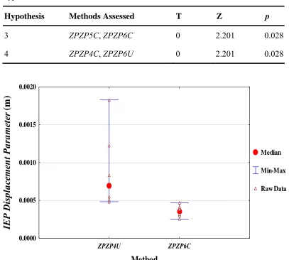
Figure 33. Range plot showing the median, range and raw data points of the IEP Displacement Parameter values across the six trials assessed in this research, for unconventional method ZPZP4U and conventional

method ZPZP6C. 166

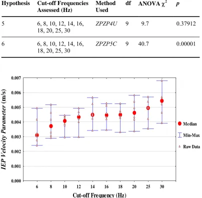
Figure 34. Range plot showing the median, range and raw data points of the IEP Velocity Parameter values for the ZPZP5C method, across the six trials assessed in this research, that resulted when the supplied data were smoothed at various cut-off frequencies (ANOVA χ2_{[df = 9,}

N = 6] = 40.7, p = 0.00001). 168

ZPZP5C method (trial ‘4466’) for force data low-pass filtered at

30 Hz. 169 Figure 36. Plot of CM[y]IA(t) and COP[y](t) with IEPs resulting from the

ZPZP5C method (trial ‘4466’) for force data low-pass filtered at 6 Hz. 169 Figure 37. Plots of COP[y](t) (labelled COP) and CM[y]IA(t) (labelled

GLP), reprinted and adapted from figure 5 of King and Zatsiorsky

(2002), with permission of Elsevier. The inset magnification shows instances between approximately 18 to 19 s when the CM[y]IA(t) plot is

not smooth, inferring CM′[y]IA(t) is not continuous at these points in

time. 174

(16)

phase of a typical trial captured in this study. Note that Fz does not

return to zero during the airborne phase. 211

Figure 39. Range plots of Quasi-static and Airborne RMS CM[z]IA-SK

Parameter values (Eq. (39) and Eq. (40), respectively) across six trials assessed in this research, for each of the four vertical dimension IA optimisation methods, illustrating the relationship between relative CM[z]IA and CM[z]SK values is significantly closer during the

quasi-static phase compared to the airborne phase. 213

Figure 40. Plots of relative CM[z]IA(t) and relative CM[z]SK(t) for a typical

countermovement jump (trial ‘5208’). Only IA optimisation

Methods AMax and BMax are shown up to and including the airborne

phase. The end of the defined quasi-static phase is indicated (tQSfin). 214

Figure 41. Plots of relative CM[z]IA(t) and relative CM[z]SK(t) for the

airborne phase of the same trial as Fig. 40 (trial ‘5208’). All four vertical dimension IA optimisation methods are shown, with A2000 and B2000 CM[z]IA(t) plots offset relative to the AMax and BMax plots

(the offset procedure is explained on page 218 and the rationale for its application is depicted clearly in Fig. 42. Peak Height differences between IA methods of up to 9.2 mm are depicted, with 14.9 mm

between the SK method and Method AMax. 215

Figure 42. Plots of relative CM[z]IA(t) and relative CM[z]SK(t) for the

quasi-static phase and the start of the countermovement phase of trial ‘5208’. The A2000 and B2000 relative CM[z]IA(t) plots are

adjusted with respect to the AMax and BMax plots, as described in the above text, to enable a valid graphical comparison. The start of the quasi-static phases, as defined by the Max and 2000 methods, and the end of the quasi-static phase, which has a common definition in both methods, are shown here as tQSini (Max), tQSini (2000) and tQSfin (both),

respectively. 218 Figure 43. Plots of relative CM[z]IA(t) and relative CM[z]SK(t) for the

airborne and landing phases of the same trial as Figs. 40, 41 and 42 (trial ‘5208’). The A2000 and B2000 relative CM[z]IA(t) plots are

adjusted with respect to the AMax and BMax plots, as described on page 218. The start and finish of the airborne phase are indicated by

tABini and tABfin, respectively. 219

Figure 44. Range plot showing the median, range and raw data points of the Quasi-static RMS CM[y]IA-SK Parameter values (Eq. (37)) across

the six trials assessed in this research, for the three antero-posterior

dimension IA optimisation methods (ANOVA χ2

[df = 2,

(17)

quasi-static phases, as defined by the BMax, B2000 and ZPZP5U methods, are shown here as tQSini (BMax), tQSini (B2000) and tQSini (ZPZP5U),

respectively. 223 Figure 46. Plots of relative CM[y]IA(t) and relative CM[y]SK(t) for the

quasi-static, countermovement and airborne phases for the same trial as depicted in Fig. 45 (trial ‘5210’). The ZPZP5U and B2000 relative CM[y]IA(t) plots are adjusted with respect to the BMax plot, as

described on page 222, to enable a valid graphical comparison. tQSini (BMax), tQSini (B2000) and tQSini (ZPZP5U) denote the start of the

quasi-static phases, as defined by the three antero-posterior [y]

methods. The end of the quasi-static stance phase (tQSfin) is also

shown, as are the start and finish of the airborne phase (tABini and

tABfin). 224

Figure 47. Plots of relative CM[z]SK(t), relative CM[z]IA(t) and

CM′[z]SK-IA(t) for Method B2000[z] (trial ‘5209’). This full-scale

graph shows the relatively erratic behaviour of the CM′[z]SK-IA(t) plot

during the dynamic phases of the trial (shaded) and its relative

consistency during the pre- and post-jump quasi-static phases. 233

Figure 48. Zoomed plot of CM′[z]SK-IA(t) for Method B2000[z]

(trial ‘5209’), concentrating on the unshaded, pre- and post-jump quasi-static stance phases. A linear regression line fitted to the post-jump quasi-static phase data (not shown) had a gradient of -0.0052, suggesting the presence of a quadratic drift, with respect to t, in post-landing CM[z]IA(t) calculations. Trials ‘5211’, ‘5212’ and

‘5217’ produced similar results. 235

Figure 49. Zoomed plot of CM′[y]SK-IA(t) for Method ZPZP5U[y]

(trial ‘5212’), concentrating on the unshaded, pre- and post-jump quasi-static stance phases. A linear regression line fitted to the post-jump quasi-static phase data (not shown) had a gradient of -0.0011, suggesting the presence of a subtle quadratic drift, with respect to t, in post-landing CM[y]IA(t) calculations. Trials ‘5209’ and

‘5217’ produced similar results but with progressively more

pronounced quadratic drifts (see also Fig. 51 for trial ‘5217’). 236

Figure 50. Zoomed plot of CM′[y]SK-IA(t) for Method ZPZP5U[y]

(trial ‘5211’), concentrating on the unshaded, pre- and post-jump quasi-static stance phases. A linear regression line fitted to the post-jump quasi-static phase data had an essentially negligible gradient of -0.0001 and a mean value, essentially, of zero, suggesting the presence of no drift or, possibly, a subtle linear or quadratic drift,

with respect to t, in post-landing CM[y]IA(t) calculations. 237

Figure 51. Plot (not zoomed in) of CM′[y]SK-IA(t) for Method ZPZP5U[y]

(trial ‘5217’), concentrating on the unshaded, pre- and post-jump quasi-static stance phases. A linear regression line fitted to the post-jump quasi-static phase data had a gradient of 0.0288, suggesting the presence of a quadratic drift, with respect to t, in post-landing CM[y]IA(t) calculations. This plot was not zoomed to the same scale as

(18)

CM′[y]SK-IA(t). A larger scale was also required for the left axis

because this trial was the broad jump. 238

Figure 52. Two of the possible five orders of progression of entire body IDA calculations for the model used in this research. Arrows indicate the directions in which the IDA calculations proceed. The left figure illustrates how an IDA commencing with Distal-to-Proximal (DP) calculations for the limbs leads to Proximal-to-Distal (PD) net force and moment calculations for the trunk-neck joint, the head-neck joint and the vertex of the head. The right figure shows how commencing with DP calculations for the non-supported ‘extremities’ leads to PD net force and moment calculations for the hip, knee and ankle joints and the distal end of the support leg. Once IDA calculations have been conducted through the entire body using all five possible orders of progression (i.e. one terminating at each of the five ‘extremities’), a pair of PD and DP net forces and moments has been calculated for all

joints and distal segment end-points. 270

Figure 53. A free body diagram of a segment and the 2-D components of the net joint forces (Fy and Fz) and the moments (Mx) acting on the segment at both its commencing and terminating end-points of the IDA (viz. Comm and Term). The 2-D position coordinates of Comm and Term and of the segmental centre of mass are bracketed and shown in

red. 271

Figure 54. A two-segment system (left box), linked at the joint inside the grey circle. The main part of the figure, showing the free body diagrams of both segments, illustrates the bi-directional (DP and PD) IDA calculations possible at the joint linking both segments. FyTermA(DP), FzTermA(DP) and MxTermA(DP) are the net external force

and moment acting at point TermA, as determined by a DP IDA of segA. FyTermB(PD), FzTermB(PD) and MxTermB(PD) are the net external

force and moment acting at point TermB, as determined by a PD IDA of segB. For a theoretically perfect system, these kinetic quantities are

equal and opposite. That is, FyTermA(DP) + FyTermB(PD),

FzTermA(DP) + FzTermB(PD) and MxTermA(DP) + MxTermB(PD) should all

equal zero. 273

Figure 55. The minimised objective function values of objective functions IDAFoot, IDAFoot and IDAAll (Foot, Hip and All, respectively), under

each of the four kinematic data filtering conditions (70%GCV,

80%GCV, 90%GCV and GCV). 284

(19)

All_2, respectively), under each of the four kinematic data filtering

conditions (70%GCV, 80%GCV, 90%GCV and GCV). 286

Figure 58. The percentage of all 64 cases (i.e. 4 trials × 4 objective functions × 4 filtering conditions) for which each BSP’s lower and

upper bound constraints became active. 288

Figure 59. The minimised objective function values of objective functions IDAFoot, IDAHip, IDAAll and IDAAll_2 (Foot, Hip, All and All_2,

respectively) for trials A and B, under each of the four kinematic data

filtering conditions (70%GCV, 80%GCV, 90%GCV and GCV). 289

Figure 60. The minimised objective function values of objective functions

IDAFoot, IDAHip, IDAAll and IDAAll_2 (Foot, Hip, All and All_2,

respectively) for trials C and D, under each of the four kinematic data

filtering conditions (70%GCV, 80%GCV, 90%GCV and GCV). 290

Figure 61. The number of active BSP bound constraints for the four kinematic data filtering conditions (70%GCV, 80%GCV, 90%GCV and GCV), for each of the objective functions (IDAFoot, IDAFoot, IDAAll

and IDAAll_2). 290

Figure 62. Oblique view of the surface map of feasible ZPZP4U solutions, with respect to Eqs. (25), in the FzC-MxO subspace (trial ‘4461’),

showing the relative insensitivity of the objective function to the

broadly feasible range of FzC and MxO perturbations (0.121 mm

difference; cf. Figs. 63 and 64). 334

Figure 63. Oblique view of the surface map of feasible ZPZP4U solutions, with respect to Eqs. (25), in the FzC-FyO subspace (trial ‘4461’). The

relative insensitivity and sensitivity, respectively, of the objective function to feasible perturbations of FzC and FyO is indicated by the

plotted surface: a valley with steep sides in the FyO dimension but

relatively negligible slope in the FzC dimension. 334

Figure 64. Oblique view of the surface map of feasible ZPZP4U solutions, with respect to Eqs. (25), in the FyC-FyO subspace (trial ‘4461’). The

sensitivity of the objective function to feasible perturbations of both FyC and FyO is indicated by the plotted surface: a valley with steep

sides in both the FyC and FyO dimensions and a long axis, with

essentially zero slope, projected diagonally onto the FyC-FyO plane. 335

Figure 65. Same surface map as in Fig. 64, but now as viewed from ‘side-on’ at (FyC, FyO, Objective-Function) = (1, 2.23, 0), indicating

the relatively negligible change along the valley’s long axis

(< 0.023 mm difference for trial ‘4461’). 335

Figure 66. The relationship between FyO and the subsequent number of

IEPs and the ZPZP4U objective function value for a typical quiet

stance trial (‘4461’). 345

Figure 67. Non-feasible CM[y](t) and COP[y](t) resulting from the

application of ZPZP4U (trial ‘4461’) with FyO assigned a value

of -0.5 N, well below its feasible range, with respect to Eqs. (25), of

(20)

application of ZPZP4U (trial ‘4461’) with FyO assigned a value of

1.44 N, still somewhat below its feasible range, with respect to

Eqs. (25), of 1.489 to 1.515 N. 346

1.52 N, just above its feasible range, with respect to Eqs. (25), of 1.489

to 1.515 N. Note that min(CM[y](t)) is just less than min(COP[y](t)). 347 Figure 70. Non-feasible CM[y](t) and COP[y](t) resulting from the

3.8 N, well above its feasible range, with respect to Eqs. (25), of 1.489

to 1.515 N. 347

Figure 71. ‘Corrected’ Fy (trial ‘4461’) with FyO assigned a value well

above its feasible range (3.8 N). The ZPs are marked with squares.

See related Fig. 70. 348

Figure 72. ‘Corrected’ Fy (trial ‘4461’) with FyO assigned a value just

above its feasible range (1.52 N). The ZPs are marked with squares.

(21)

Table 8. The three core approaches to IA optimisation developed and assessed in this experiment (column 1). Column 2 indicates each specific method formulated under each basic category, based on different definitions of the duration of the quasi-static stance phase. The dimension and the design variables relevant to each method’s objective function are indicated in columns 3 and 4, respectively. Design variables TOL

List of Tables

Table 1. Segment definitions in terms of the various markers (actual and virtual) used to represent the distal and proximal segment end-points. Virtual markers are subscripted with an A, B, or C, reflecting one of the three different methods applied to derive such markers (see

section 4.4.1.1). Inferior and superior trunk end-points were

considered proximal and distal, respectively. L/R refers to left or

right. 123

Table 2. Joint definitions in terms of the various actual and virtual markers used and derived, respectively, to represent the joint centres. Virtual markers are subscripted with an A, B, or C, reflecting one of the three different methods applied to derive such markers (see section 4.4.1.1). For any joint centre that was, by definition, co-located with one or more of the defined segment end-point locations, such end-points are listed in parentheses. Inferior and superior trunk end-points were considered proximal and distal,

respectively. L/R refers to left or right. 124

Table 3. The bound constraints initially applied to the proposed design variables, but later rejected, based on the sensitivity analyses (see Appendix A). Also shown are the initial estimates of the proposed design variables that were used for all ZPZP4U and ZPZP5C

optimisations. 145 Table 4. Summary of all the ZPZP methods assessed in this experiment.

Methods with the suffix C denote ‘conventional’ methods, in which the ZPZP algorithm (see page 17) was applied in the conventional manner across each and every ZPZP interval, as per Zatsiorsky and Duarte (2000). Methods with the suffix U denote ‘unconventional’ methods, in which the ZPZP algorithm was applied in an unconventional manner once only across the entire interval spanned by the initial and

final identified ZPs. 148

Table 5. Results of the Friedman rank-order ANOVA tests (N = 6) used

to assess Hypotheses 1 and 2. 153

Table 6. Results of the Wilcoxon matched pairs tests (N = 6) used to

assess Hypotheses 3 and 4. 166

to assess Hypotheses 5 and 6. 168

0 and TOLfin are defined in section 6.1.1.1 on

(22)

Table 9. Median and range values for the duration of the quasi-static phase for all variable-duration methods (N= 6). By definition, the other methods (A2000[z], B2000[z] and B2000[y]) all had quasi-static

phases with a set duration of 2000 ms. 212

to assess the vertical IA optimisation methods (Hypotheses 7 and 8). 213

Table 11. Jump performance parameters HeightJ and HeightP that

resulted from the application of each of the vertical dimension IA methods for all six trials, and the maximum between-method differences expressed in absolute terms (mm) and as a percentage (%) of the maximum parameter value produced for that trial (the bolded result in the relevant row). It is evident that no particular method consistently produced the largest or smallest values across all trials. 216

Table 12. Jump performance parameters WorkP, Max PowerP and

Ave PowerP that resulted from the application of each of the vertical

dimension IA methods for all six trials, and the maximum between-method differences expressed in absolute terms (J/kg or W/kg) and as a percentage (%) of the maximum parameter value produced for that trial (the bolded result in the relevant row). It is evident that no particular method consistently produced the largest or smallest values across all, or even most trials for these parameters. 217 Table 13. Results of the Friedman rank-order ANOVA tests (N = 6) used

to assess the antero-posterior IA optimisation methods (Hypotheses 9

and 10). 221

Table 14. For Methods A2000[z] and B2000[z], the maximum, mean and SD of the changes (∆) in the jump performance parameters HeightJ,

HeightP, WorkP, Max PowerP and Ave PowerP (all defined in

section 6.1.2.3) across all trials, produced by setting CM′[z]IA(0) to

zero (Condition 2). These changes are expressed in absolute terms (mm, J/kg or W/kg) and, except for SD, as percentages (%) of the parameter values derived from the originally optimised solutions

(Condition 1). Negative values denote reductions. 226

Table 15. For Methods A2000[z] and B2000[z], the maximum, mean and SD of the changes (∆) in the jump performance parameters HeightJ,

HeightP, WorkP, Max PowerP and Ave PowerP (all defined in

section 6.1.2.3) across all trials, produced by perturbing the originally

optimised FzO value by +1 N (Condition 3). These changes are

(23)

SD, as percentages (%) of the parameter values derived from the originally optimised solutions (Condition 1). Negative values denote

reductions 230 Table 17. For Methods A2000[z] and B2000[z], the maximum, mean and

SD of the changes (∆) in the generic parameter Peak Height (defined in section 6.1.2.4) across all trials, produced by setting CM′[z]IA(0) to

zero (Condition 2), perturbing the originally optimised FzO value by

+1 N (Condition 3), and including mWB as a design variable and

setting FzO to zero (Condition 4). These changes are expressed in

absolute terms (mm) and, except for SD, as percentages (%) of the parameter values derived from the originally optimised solutions

(Condition 1). Negative values denote reductions. 231

Table 18. Gradients of the linear regression lines fitted to the CM′SK-IA(t)

data separately for the pre- and post-jump quasi-static (QS) phases

across the four relevant trials for Methods B2000[z] and ZPZP5U[y]. 234 Table 19. The initial values and lower and upper bound constraints

applied to each of the mseg and Iseg BSP design variables included in

the optimisations. Each segment’s mass (mseg) is expressed as a

proportion of whole body mass (mWB) and the principal segmental

moments of inertia about the subject’s transverse axis through each

segment’s centre of mass (Iseg) are expressed in kgm2. 263

Table 20. The initial values and lower and upper bound constraints applied to each of the segmental centre of mass BSP design variables. Each segment’s longitudinal and perpendicular segmental centres of mass (cm[L]seg and cm[P]seg) are expressed as proportions of segment

length. 264 Table 21. The design variable coordinates for which absolute and relative

COP[y](ti) and CM[y]IA(ti) parameters were calculated. Cases with

shaded cells in the same column were used to assess the sensitivity of these parameters to perturbations in each corresponding design

variable. (wrt = ‘with respect to’). 340

Table 22. Results of sensitivity analyses showing the largest differences observed across all trials for each of the relative and absolute parameters ∆ABS1, ∆ABS2, ∆REL1, ∆REL2, and RMS REL3. All measures are in metres. Negative values in the ∆REL1 and ∆REL2

columns indicate that these relative parameters increased as the relevant design variable increased. See Table 21 for definitions of

(24)

List of Equations

Equation (1) 12

Equation (2) 12

Equation (3) 13

Equation (4) 13

Equation (5) 13

Equations (6) 15

Equation (7) 33

Equation (8) 33

Equation (9) 40

Equation (10) 72

Equation (11) 72

Equation (12) 80

Equation (13) 80

Equations (14) 80

Equations (15) 131

Equation (17) 132

Equation (20) 134

Equation (23) 141

Equation (24) 143

Equation (27) 146

(25)

Equation (33) 193

Equation (34) 193

Equation (35) 197

Equation (36) 199

Equation (37) 203

Equation (38) 203

Equation (39) 203

Equation (40) 203

Equation (41) 207

Equation (42) 207

Equation (43) 207

Equation (46) 266

Equation (47) 267

Equation (48) 267

Equation (49) 267

Equation (50) 268

Equation (51) 269

Equation (52) 269

Equation (53) 269

Equation (54) 272

Equation (55) 272

Equation (56) 272

Equation (57) 274

Equation (58) 274

Equation (59) 274

Equation (60) 276

Equation (61) 276

(26)

Acronyms and Abbreviations

2-D Two-dimensional

3-D Three-dimensional

AOJ Atlanto-Occipital Joint

AVI Audio Video Interleave

BSP Body Segment Parameter

CCTV Closed Circuit Television

CM Whole Body Centre of Mass

COP Centre of Pressure

CT Computed Tomography (also known as Computed Axial

Tomography, or Computer Aided Tomography)

DEXA Dual Energy X-ray Absorptiometry (also referred to as DXA)

DP Distal-to-Proximal (IDA calculations) (see page 270)

ESU Event Synchronisation Unit

FDA Forward Dynamics Approach (see page 3)

GCV Generalised Cross-Validation (see page 129)

GRF Ground Reaction Force

HAT Head-arms-trunk (segment)

HCM Whole body angular momentum about the CM

H′CM Rate of change of HCM, with respect to time

(27)

LED Light Emitting Diode

MRI Magnetic Resonance Imaging

OTNJ Optimised Trunk-Neck Joint (see page 120)

PD Proximal-to-Distal (IDA calculations) (see page 270)

RMS Root-mean-square

SD Standard Deviation

SE Standard Error

SK Segmental Kinematic (see page 3)

TNJ Trunk-Neck Joint

TTL Transistor-transistor Logic

ZP Zero-point (see page 17)

(28)

Notation

Note: Only the notation used in this research is included in this table. Notation

presented by other authors is sometimes reproduced in the text for illustrative

purposes, but it is not summarised in this table. Commonly used subscripts, such

as i, that were simply used to define iterative processes that applied to a particular

equation or sequence of equations locally within the text are also not listed in this

table. Such subscripts may have been used independently in different sequences

of equations, so they are only defined locally within the text.

Ave PowerP Average vertical translational power per kilogram of

body mass for the upward propulsive phase of a

countermovement jump (see section 6.1.3)

cmseg Centre of mass position of segment ‘seg’ (e.g. cmfoot)

cm[L]seg Centre of mass coordinate of segment ‘seg’ along the

longitudinal axis (L) in the segment-based reference

system (see Fig. 12)

cm[P]seg Centre of mass coordinate of segment ‘seg’ along the

perpendicular axis (P) in the segment-based reference

system (see Fig. 12)

CM(t) Whole body centre of mass displacement as a function of

(29)

CMIA(t) CM(t) determined using force platform data and an IA

CM′IA(t) CMʹ(t) determined using force platform data and an IA

CMSK(t) CM(t) determined using full body SK data and a weighted

average of segmental centre of mass estimates

CM′SK(t) CM′(t) determined using full body SK data and a

weighted average of segmental centre of mass velocity

estimates

CM′SK-IA(t) CM′SK(t) - CM′IA(t)

CM[y]IA(t) Antero-posterior component of CMIA(t) (in Chapters 5

and 6)

CM′[y]IA(t) Antero-posterior component of CM′IA(t) (in Chapters 5

and 6)

CMy Horizontal coordinate of the CM position vector in the

global coordinate system (in Chapter 7)

cm[y]seg Horizontal component [y] of the displacement of the

centre of mass of segment ‘seg’ in the global coordinate

system

cm[y′]seg Horizontal component [y] of the velocity of the centre of

mass of segment ‘seg’ in the global coordinate system

cm[y′′]seg Horizontal component [y] of the acceleration of the centre

of mass of segment ‘seg’ in the global coordinate system

CM[z]IA(t) Vertical component of CMIA(t) (in Chapters 5 and 6)

CM′[z]IA(t) Vertical component of CM′IA(t) (in Chapters 5 and 6)

(30)

of mass of segment ‘seg’ in the global coordinate system

cm[z′]seg Vertical component [z] of the velocity of the centre of

cm[z′′]seg Vertical component [z] of the acceleration of the centre of

Comm Commencing end of the segment undergoing an IDA (see

page 271)

Comm[y] Horizontal position of the commencing end of the

segment undergoing an IDA (see page 271), with respect

to the global coordinate system origin

Comm[z] Vertical position of the commencing end of the segment

undergoing an IDA (see page 271), with respect to the

global coordinate system origin

COP[y] Antero-posterior component of the centre of pressure

location (in Chapters 5 and 6)

COPy Horizontal coordinate of the COP position vector in the

global coordinate system (in Chapter 7)

Dist[y]seg The horizontal component [y] of the position of the distal

end-point of segment ‘seg’ in the global coordinate

system

Dist[z]seg The vertical component [z] of the position of the distal

(31)

f Frequency of data sampling (1/∆t)

FC Force platform calibration factor error in F (see page 31)

FO Force platform offset error in F (see page 33)

Fy Antero-posterior component of the net ground reaction

force measured by the force platform

FyC Force platform calibration factor error term for Fy

FyComm Horizontal component of the net force acting on the

commencing end (Comm) of the segment in question in

an IDA (see page 271)

FyO Force platform offset error term for Fy

FyTerm Horizontal component of the net force acting on the

terminating end (Term) of the segment in question in an

IDA (see page 271)

Fz Vertical component of the net ground reaction force

measured by the force platform

Fz Quasi-static mean Fz (see page 197)

FzC Force platform calibration factor error term for Fz

FzComm Vertical component of the net force acting on the

commencing end (Comm) of the segment in question in

an IDA (see page 271)

FzO Force platform offset error term for Fz

FzTerm Vertical component of the net force acting on the

terminating end (Term) of the segment in question in an

(32)

g Acceleration due to gravitational force, which

was -9.80 ms-2_{at sea level in Melbourne, Australia}

(International Society of Geodesy, 1971), where the

research was conducted

HeightJ Jumping height, representing the increase in vertical CM

displacement from take-off to the peak of CM flight (see

section 6.1.3)

HeightP Increase in vertical CM displacement from the minimum

point in the countermovement to the take-off point during

a countermovement jump (see section 6.1.3)

IEPi ith IEP in a sequence of IEPs

IEPn Final IEP in a sequence of IEPs

IEP0 Initial IEP in a sequence of IEPs

Iseg Moment of inertia (assumed to be the principal moment

of inertia) of segment ‘seg’, about the transverse axis

through the segment’s centre of mass

L The longitudinal axis of the segment-based reference

system (see page 125 and Fig. 12).

lseg Length of the segment ‘seg’

mWB Whole body mass

Mx Measured moment about the x-axis of the force platform

(33)

page 271)

MxO Force platform offset error term for Mx

MxComm Net moment acting about the x-axis at the commencing

end (Comm) of the segment in question in an IDA (see

page 271)

mseg Mass of segment ‘seg’

Max PowerP Maximum vertical translational power per kilogram of

body mass during the upward propulsive phase of a

countermovement jump (see section 6.1.3)

P Perpendicular axis of the segment-based reference system

(see page 125 and Fig. 12)

Peak Height Height of the CM at the peak of CM flight trajectory,

relative to the height of the CM at the start of the

pre-jump quasi-static phase (RelCM[z]IA(tPH))

Prox[y]seg The horizontal component [y] of the position of the

proximal end-point of segment ‘seg’ in the global

coordinate system

Prox[z]seg The vertical component [z] of the position of the proximal

end-point of segment ‘seg’ in the global coordinate

system

seg

rv Position vector of the segmental centre of mass relative to

the global coordinate system origin

seg

r&&v Second derivative of rv_seg

(34)

RelCMSK(t) Relative CMSK(t); that is, CMSK(t) relativeto CMSK(tQSini)

S0 IA parameter representing the initial displacement of the

CM

0 ˆ

S Estimated S0

Sε Error in estimated S0

S[y]0 IA parameter representing the initial absolute

antero-posterior displacement of the CM [the y coordinate

of CM(0)IA]

S[z]0 IA parameter representing the initial absolute vertical

displacement of the CM [the z coordinate of CM(0)IA]

Tx(t) Net torque about the x-axis produced by the whole body

weight force acting at the CM, and the GRF acting at the

COP, with respect to the global coordinate system origin

Term[y] Horizontal position of the terminating end of the segment

Term[z] Vertical position of the terminating end of the segment

t Time

tABini Time of commencement of the airborne (AB) phase of a

(35)

ti ith instant in a time series

tmaxCMy Time at which max(CM[y]IA(t)) occurs (see page 143)

tminCMy Time at which min(CM[y]IA(t)) occurs (see page 143)

tPfin Time of completion of the upward propulsive phase of a

countermovement jump (see page 206)

tPini Time of commencement of the upward propulsive phase

of a countermovement jump (see page 206)

tPH Time coinciding with the peak of CM flight trajectory

tQSfin Time of completion of the pre-jump quasi-static (QS)

stance phase of a countermovement jump (see page 192)

tQSini Time of commencement of the pre-jump quasi-static (QS)

stance phase of a countermovement jump (see page 192)

Tx Net external torque acting on the body with respect to the

TOLfin Tolerance in final IEP (design variable in ZPZP5U; see

page 194)

TOLi Tolerance in IEPi (design variables in ZPZP6C; see

page 146)

TOL0 Tolerance in initial IEP (design variable in ZPZP5U; see

page 194)

V0 IA parameter representing the initial velocity of the CM

0 ˆ

V Estimated V0

Vε Error in estimated V0

(36)

velocity of the CM [the y coordinate of CMʹ(0)IA]

V[z]0 IA parameter representing the initial vertical velocity of

the CM [the z coordinate of CMʹ(0)IA]

WorkP Vertical translational work done per kilogram of body

mass in accelerating the CM upwards during the upward

propulsive phase of a countermovement jump (see

section 6.1.3)

seg

y&& Horizontal linear acceleration of the segmental centre of

mass (see page 267)

seg

z&& Vertical linear acceleration of the segmental centre of

mass (see page 267)

αseg Angular segmental acceleration of segment ‘seg’

∆Ave PowerP (Condition i) Ave PowerP under Condition i, relative to that under

Condition 1 (see page 209)

∆HeightJ (Condition i) HeightJ under Condition i, relative to that under

∆HeightP (Condition i) HeightP under Condition i, relative to that under

∆Max PowerP (Condition i)Max PowerP under Condition i, relative to that under

(37)

∆WorkP (Condition i) WorkP under Condition i, relative to that under

Γ The distance in the sagittal plane between two given

trunk markers (see Fig. 10)

θseg Angular segmental displacement of segment ‘seg’

(38)

Unit Symbols

cm centimetre

Hz hertz

J joule

kg kilogram

m metre

mA milliampere

mcd millicandela

mm millimetre

mrad millirad

ms millisecond

mSv millisievert

N newton

s second

V volt

(39)

1. INTRODUCTION

Human biomechanics research provides a wealth of practical benefits to society,

spanning medical, clinical, occupational, sporting and artistic domains. It

encompasses the measurement, description, explanation and prediction of human

mechanics from the cellular level to whole body mechanics. A myriad of research

approaches of broadly varying complexity are applied across this field of

endeavour. Quantitative techniques range from relatively simple temporal

measurements to high-precision acquisition of total system kinematics and

kinetics. Mathematical modelling and simulation approaches of vastly different

levels of sophistication are employed.

By finding the correct balance between simplicity and complexity, researchers can

apply the most efficient yet effective measurement and modelling tools for

achieving their specific research objectives. Whole body motion, for example, is

complex by nature of the inherently intricate structural and functional design of

the human musculoskeletal system. In order to analyse this motion, researchers

often model the human as a simplified system of rigid segments linked by

frictionless joints that are spanned by several muscles. For many applications, it

is possible to simplify the model further. This may involve reducing the analysis

of each joint to a net force and moment when knowledge about the individual

contribution of each muscle is not required. Sometimes 2-D analysis is deemed

sufficient for essentially planar human performance and occupational activities

such as countermovement jumps (e.g. Kibele, 1998) and some manual lifting tasks

(40)

A kinematic representation of a human’s segmental motion is possible when the

complete position-time history of the model’s joint centres and segment

end-points is known as a result of stereophotogrammetric recording of the

human’s movement. Under certain conditions, subsequent kinetic analysis can be

conducted to estimate the external forces acting on the human body and the

internal net joint forces and moments that govern the measured kinematics. The

process of calculating such kinetic quantities by first measuring the resultant

kinematics is commonly called the inverse dynamics approach (IDA).

For non-support and single-support open-loop situations (Vaughan et al., 1982b),

only the kinematic data described above and the inertial properties of the

segments need to be supplied to the system of motion equations in order to

calculate body kinetics using the IDA. For open-loop situations involving n

extremities in contact with the external environment, force transducing devices are

also required to measure the external forces acting on at least n-1 of the

extremities if the IDA is to be applied (Vaughan et al., 1982b). Therefore, if the

number of force transducing devices used equals the number of extremities in

contact with the external environment, the system of motion equations is

over-determined. In such circumstances, the external force acting at the distal end

of any stipulated extremity can be calculated by an inverse dynamics analysis and

(41)

The opposite approach to solving dynamics equations is called the direct or

forward dynamics approach (FDA). The FDA is commonly applied in human

movement simulation studies. It involves determining the system kinematics by

providing the equations of motion with the forces and moments that drive the

model. IDA and FDA solutions also rely on the provision of the model’s

segmental inertial properties.

Segmental inertial properties or body segment parameters (BSPs) include each

segment’s mass, centre of mass position and inertia tensor. For 2-D dynamics

analysis of motion that is assumed to occur exclusively in the anatomical sagittal

plane, only each segment’s mass (mseg), centre of mass location in the sagittal

plane (cmseg) and principal moment of inertia about the transverse axis through the

segment’s centre of mass (Iseg) are required1.

When system kinematics have been captured by stereophotogrammetric means

and BSP estimates are available, it is also possible to estimate whole body centre

of mass (CM) trajectory by determining the weighted average of all the segments’

centre of mass positions for each sampled point in time (Winter, 1990). This can

be referred to as segmental kinematic (SK) determination of CM kinematics. The

1 Strictly speaking, the segmental moments of inertia about the anatomical axes are only principal

moments of inertia if the principal axes of inertia and the anatomical axes are aligned. All 2-D

human dynamics studies reviewed by the author have assumed alignment of these axes, either

(42)

whole body angular momentum about the CM (HCM) can also be calculated (Hay

et al., 1977).

All of the approaches described thus far require BSP data. Except for FDA

simulations, they also require the complex and time-consuming process of

measuring segmental kinematics. However, relatively inexpensive and less

time-consuming strategies for determining CM kinematics have been developed

that require minimal or no segmental kinematics data acquisition or BSP

estimation. Such strategies have been applied to posturographic (e.g. Benda et al.,

1994; Caron et al., 1997), gait (e.g. Crowe et al., 1993; Eames et al., 1999;

Whittle, 1997) and other movement (e.g. Hatze, 1998; Zok et al., 2004) analyses.

Essentially, they involve the reduction of the data obtained with one or more force

platforms for single-stance or double-stance open-loop situations, with little or no

reliance on kinematic measurements. For example, the integration approach (IA)

can be used if the only external forces acting on the body are gravitational force

and ground reaction forces acting on the feet as measured by one or two force

platforms. This approach involves calculating the acceleration-time history of the

CM from the ground reaction force (GRF) data, and twice integrating this data

numerically, with respect to time, in order to determine the velocity-time and

position-time histories of the CM (e.g. Kibele, 1998; Rabuffetti and Baroni, 1999;

Zatsiorsky and King, 1998). The two integration constants formed by this

(43)

The accuracy of CM kinematic data calculated using the Integration Approach

(IA) is dependent upon the accuracy of:

• kinetic data acquisition, reduction and smoothing tools and techniques

• assumed or estimated values of the integration constants.

Many variations of the IA have been proposed over recent years. An assessment

of the relative merits of these techniques and the possible refinement and

amalgamation of the most promising aspects of these methods is warranted.

Similarly, the accuracy of a variety of human biomechanics data provided by

whole body segmental modelling approaches depends upon the accuracy and

validity of:

• data acquisition, reduction and smoothing techniques

• the model developed to describe the mechanical structure and function of the

human (including the estimated BSPs, joint centres and segment end-points).

The use of subject-specific BSP estimates in human movement analysis has been

advocated (Pearsall and Reid, 1994; Reid and Jensen, 1990) in order to reduce this

error source. However, only a few currently available methods approach

subject-specificity, and direct measurement techniques are not easily and readily

applied (Zatsiorsky, 2002).

Clearly, reducing the magnitude of some or all of the abovementioned error

sources will improve biomechanical representation, explanation and simulation of

human movement. Notwithstanding the desirability of minimising all error

(44)

• improve estimation of sagittal plane CM kinematics by applying variations of

the IA, and

• improve segmental modelling for whole body sagittal plane dynamics

analyses by applying new subject-specific BSP estimation techniques.

A précis of this research follows:

The Problem: Dynamics analyses of human movement are limited by inaccurate

input parameters, such as erroneous force platform calibration parameters, IA

integration constants and BSP estimates.

The Aims: This research aims to improve the accuracy of these input parameters

and subsequently, to improve the IA CM kinematics calculations and

BSP-dependent dynamics solutions.

The Approach: Nonlinear optimisation is the key methodological approach

underpinning attempts to achieve these aims. The experimental design ensures

that enough sources of measurable data are captured to produce a complete or an

over-determined system of dynamics equations. This situation is then exploited

by applying optimisation searches to find the activity-specific and subject-specific

input parameter values that produce the dynamics solutions that most closely

correspond to the empirically-measured data (e.g. force platform measurements),

mathematically-calculated data (e.g. SK determination of CM trajectory) or

Estimating Centre of Mass Trajectory and Subject-Specific Body Segment Parameters Using Optimisation Approaches