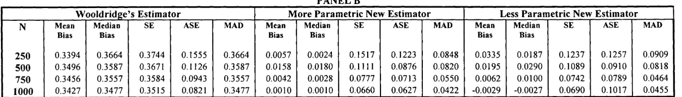
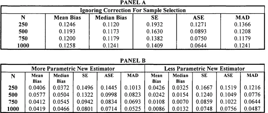
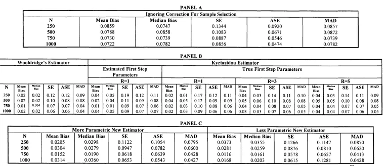
Panel data sample selection models.

(1)

Panel Data

Sample Selection Models

Maria Engracia Rochina Barrachina

Thesis submitted for the Degree of

Doctor of Philosophy in Economics

University College London

University of London

(2)

ProQ uest Number: U6 4 2 8 4 8

INFORMATION TO ALL U SE R S

The quality of this reproduction is d ep en d en t upon the quality of the copy subm itted.

In the unlikely even t that the author did not sen d a com plete manuscript

and there are m issing p a g e s, th e se will be noted. Also, if material had to be rem oved, a note will indicate the deletion.

uest.

ProQ uest U 6 4 2 8 4 8

Published by ProQ uest LLC(2016). Copyright of the Dissertation is held by the Author.

This work is protected against unauthorized copying under Title 17, United S ta tes C ode. Microform Edition © ProQ uest LLC.

ProQ uest LLC

789 East E isenhow er Parkway P.O. Box 1346

(3)

Preface

This thesis is the result o f my research activities at the Department o f Economics at

University College London (UCL), at which I have been working as a Ph.D. student. I

would like to thank some people and institutions that have supported me, and have

somehow contributed to my work.

First o f all, I would like to express my thanks to my parents, relatives and

friends for their support and encouragement. I would specially like to mention my

grandmother, which company I could only enjoy for one year more after my stay in

London.

The supervision o f both Richard Blundell and Costas Meghir is gratefully

acknowledged.

Furthermore, I would like to thank all my fellow Ph.D. students and friends at

UCL for their support, their company and the pleasant atmosphere they contributed to

create. I owe special thanks to my friend and colleague Juan Alberto Sanchis-Llopis

with whom I arrived to London, I moved out o f London and I came back for

submission o f this thesis.

I would also like to thank several institutions for their support. UCL has

contributed to my work with an stimulating research environment and the great

possibility to attend seminars given by researchers o f international prestige. Financial

support from the Spanish foundation “Fundacion Ramon Areces” is gratefully

acknowledged. This institution made my Ph.D. possible and I would like to

(4)

studies in foreign countries. I am very much indebted to my department o f Applied

Economics II at the University o f Valencia, and specially to my “moral boss” there,

José Antonio Martinez-Serrano, who started the policy o f strongly encouraging young

people to go abroad for postgraduate studies. Finally, many thanks to my colleagues

and friends in this department.

(5)

Abstract

In this thesis estimators for “fixed-effects” panel data sample selection models are

discussed, mostly from a theoretical point o f view but also from an applied one.

Besides the general introduction and conclusions (chapters 1 and 6, respectively) the

thesis consists o f four main chapters. In chapter 2 we are concerned about the finite

sample performance o f Wooldridge (1995) and Kyriazidou’s (1997) estimators.

Chapter 3 introduces a new estimator. The estimation procedure is an extension o f the

familiar two-steps sample selection technique to the case where one correlated

selection rule in two time periods generates the sample. Some non-parametric

components are introduced. We investigate the finite sample performance for the

estimators in chapters 2 and 3 through Monte Carlo simulation experiments. In

chapter 4 we apply the estimators in the previous chapters to estimate the return to

actual labour market experience for females, using a panel o f twelve years. All these

estimators rely on the assumption o f strict exogeneity o f regressors in the equation o f

interest, conditional on individual specific effects and the selection mechanism. This

assumption is likely to be violated in many applications. For instance, life history

variables are often measured with error in survey data sets, because they contain a

retrospective component. We show how non-strict exogeneity and measurement error

can be taken into account within the methods. In chapter 5 we propose two

semiparametric estimators under the assumption that the selection function depends

(6)

double pairwise difference estimator” because it is based in the comparison o f

individuals in time differences. The second is a “single pairwise difference estimator”

because only differences over time for a given individual are required. We investigate

(7)

Chapter 1 Introduction

1.1 Panel Data and Sample Selection Models

In this thesis estimators for panel data sample selection models are discussed, mostly

from a theoretical point o f view but also from an applied one. The utilisation o f panel

data is commonly confronted with two problems, sample selectivity and unobserved

heterogeneity, both o f which give rise to specification bias. Sample selectivity arises

in nonrandomly drawn samples, as a result o f either self-selection by the individuals

under investigation, or selection decisions made by data-analysts. As a consequence,

in many problems o f applied econometrics, the equation o f interest is only defined for

a subset o f individuals from the overall population, while the parameters o f interest

are the parameters that refer to the whole population. Examples are the estimation of

wage equations, or hours o f work equations, where the dependent variable can only be

measured when the individual participates in the labour market. Failure to account for

sample selection is well known to lead to inconsistent estimation o f the parameters o f

interest, as these are confounded with parameters that determine the probability o f

entry into the sample.

In contrast to sample selectivity, unobserved heterogeneity is a problem

(11)

CHAPTER 1. INTRODUCTION 10

contain an individual specific effect, which is unobserved, but correlated with the

model regressors. Examples are unobserved ability components in wage equations,

correlated with wages and education (see Card (1994) for details), or the estimation o f

Frisch demand functions in the consumption and labour supply literature (see, for

instance. Browning, Deaton, and Irish (1985), Blundell and MaCurdy (1999) and

MaCurdy (1981)). If unobserved individual specific (and time constant) effects affect

the outcome variable, and are correlated with the model regressors, simple regression

analysis does not identify the parameters o f interest. In this thesis, if the individual

effects are considered as nuisance parameters or if they are explicitly allowed to

depend on the explanatory variables in a given or fully unrestricted way, then we call

the panel data model a “fixed-effects” model.

In many applications with panel data, both sample selectivity and unobserved

heterogeneity problems occur simultaneously. In this thesis we consider the problem

o f estimating panel data sample selection models with a binary selection equation.

Both the sample selection rule and the regression equation o f interest contain

permanent unobservable individual effects possibly correlated with the explanatory

variables.

The general model, which summarises the models along all the chapters in this

thesis, can be written as follows,

y„ =x^,P + a , + s „ \ i = t = \,...,T , (1.1)

(12)

C H A P T E R !. INTRODUCTION H

where x„ and are vectors o f explanatory variables (which may have components in

common), is an unknown parameter (column) vector, and are

unobserved disturbances, and and 77, are individual-specific effects presumably

correlated with the explanatory variables in the model. The index function /( • ) in

(1.2) is a scalar “aggregator” function which can accommodate different structures. In

particular, we allow either for a linear parametric form o f this function or an

unrestricted one. Whether or not observations for are available is denoted by the

dummy variable . By following an estimation procedure that just uses the available

observations one is implicitly conditioning upon the outcome o f the selection process,

i.e., upon d.^ = 1. The problem o f selectivity bias arises from the fact that this conditioning may affect the unobserved determinants o f jP/, •

For the estimators considered in this thesis the individual effects cr, and 77,

are treated as nuisance parameters or, alternatively, they are explicitly allowed to

depend on the explanatory variables in a given or fully unrestricted way. Furthermore,

each estimator imposes different stochastic restrictions for the error terms in the

model. In this thesis we are interested in the estimation o f the regression coefficients

(13)

C H A P T E R ], INTRODUCTION 1 2

1.2 Contribution of This Thesis and Overview

The contribution o f this thesis is to develop, apply, and learn about estimators for

panel data sample selection models. Besides the theoretical approach to the

estimators and the results from Monte Carlo simulations, applications can clarify the

use o f the estimators in practice.

This thesis consists o f four main chapters. In the following, each o f these

chapters is discussed only briefly since each chapter is accompanied by its own

introduction and conclusions. The emphasis is on the objectives and the interrelation

between these chapters. The last chapter, chapter 6, provides a brief summary o f the

main results and conclusions from the various chapters.

In chapter 2, we examine W ooldridge (1995) and Kyriazidou’s (1997)

estimators for "fixed-effects” panel data sample selection models. The specification

o f the function /( • ) in (1.2) is / ( ^ „ ) = z ^ j , where / e is an unknown parameter

(column) vector. For Kyriazidou’s (1997) estimator both cr, and 77, are treated as

nuisance parameters. In Wooldridge (1995) they are explicitly allowed to depend on

the leads and lags o f the explanatory variables through a linear projection operator.

Each estimation method relies on different stochastic restrictions for the error terms in

(14)

C H A P T E R ). INTRODUCTION 13

Wooldridge (1995) is focused on the simplest consistent estimator o f p in (1.1), a pooled OLS, we work with a more efficient minimum distance estimator.

Furthermore, we characterise the asymptotic distribution for the minimum distance

version o f Wooldridge’s (1995) estimator. The finite sample properties o f the

estimators are investigated by Monte Carlo experiments.

Chapter 3 is identical to Rochina-Barrachina (1999). In this chapter we

introduce a new estimator for panel data sample selection models with "fixed-effects”.

The estimator relaxes some o f the assumptions in the methods in chapter 2.

Specifically, the estimator treats a , as a nuisance parameter allowed to depend on the

explanatory variables in an arbitrary fashion, in contrast to Wooldridge (1995), and it

also avoids the conditional exchangeability assumption in Kyriazidou (1997). The new estimator can be seen as complementary to those previously suggested, in the

sense that it uses an alternative set o f identifying restrictions to overcome the selection

problem. In particular, the estimator imposes that the joint distribution o f the time

differenced regression equation error and the two selection equation errors,

conditional upon the entire vector o f (strictly) exogenous variables, is normal. The

estimation procedure is an extension o f Heckman’s (1976, 1979) sample selection

technique to the case where one correlated selection rule in two different time periods

generates the sample. The idea o f the estimator is to eliminate the individual effects

from the equation o f interest by taking time differences, and then to condition upon

the outcome o f the selection process being “one” (observed) in the two periods. This

leads to two correction terms, the form o f which depends upon the assumptions made

(15)

CHAPTER 1. INTRODUCTION 1 4

our analysis on two periods. Consequently, we get estimates based on each two waves

we can form with the whole length o f the panel, and then we combine them using a

minimum distance estimator.

We present two versions o f the estimator depending on the treatment o f the

individual effects rj^. If 7, is explicitly allowed to depend on the explanatory

variables in a linear way (as in Wooldridge (1995)) we have a version o f the estimator

referred to as the “more parametric new estimator”. In this case, f(z■^ ) - 7, in (1.2) is

assumed to be equal to - c , , where z, = (z,,,...,z,y), y, \ and c, is a random effect uncorrelated to the model regressors. However, if 77, is explicitly

allowed to depend on the explanatory variables in a fully unrestricted way we call the

estimator “less parametric new estimator”. Under this alternative approach, to allow

for semiparametric individual effects in the selection equation, the conditional mean

o f 77. is treated as an unknown function o f the whole time span o f the explanatory

variables. The finite sample properties o f both versions o f the estimator are compared

to those o f Wooldridge (1995) and Kyriazidou’s (1997) estimators by Monte Carlo

experiments. In the Appendices o f the chapter we provide formulae for the

asymptotic variance o f the new estimators.

The objective of chapter 4 is to learn about the performance o f the methods in

practice. Not many applications o f these estimators exist in the literature. The first

part o f the chapter compares the three estimators in the previous chapters, points out

(16)

Strict exogeneity o f regressors in the equation o f interest, conditional on individual

specific effects and the selection mechanism. This assumption is likely to be violated

in many applications. We show how non-strict exogeneity and measurement error can

be taken into account within the estimation methods discussed. In the second part o f

the chapter, to learn about its performance we apply the estimators and their

extensions to a typical problem in labour economics: The estimation o f wage

equations for female workers. The parameter we seek to identify is the effect o f actual

labour market experience on wages. Results for the participation equation for a

selection o f estimators are presented. The data for our empirical application is drawn

from the German Socio-Economic Panel (GSOEP). The dataset used for estimation is

based on the first 12 waves o f the panel. The problems that arise in this application

are non-random selection, and unobserved individual specific heterogeneity which

might be correlated with the regressors. In addition, actual experience is

predetermined, and the experience measure is likely to suffer from measurement error.

In chapter 5, estimation o f the coefficients in a “double-index” selectivity bias

model is considered under the assumption that the selection correction function

depends only on the conditional means o f some observable selection variables. We

present two alternative methods. The first is referred to as a “weighted double

pairwise difference estimator” (WDPDE) because o f being based in the comparison of

individuals in time differences. On the resulting model we apply a weighted least

squares regression with decreasing weights to pairs o f individuals with larger

differences in their “double index” variables, and then larger differences in the

(17)

estimator o f cross-section censored selection models to “fixed-effects” panel data

models. We call the second method a “single pairwise difference estimator” (SPDE)

because only differences over time for a given individual are required. On the model

in time differences we take out its conditional expectation on the selection variables

(the “double index”). This generalisation o f Robinson’s (1988) “partially linear”

model to the case o f panel data sample selection models with “fixed-effects” is

estimated by least squares regression.

The estimators in this chapter have similar desirable properties as the estimator

in chapter 3 (specially as the version called “less parametric new estimator”). They

treat a , as a nuisance parameter (as in Kyriazidou (1997) and our estimator in chapter

3) and rj, is explicitly allowed to depend on the explanatory variables in a fully unrestricted way (as chapter’s 3 estimator under its less parametric version).

However, they are distributionally free estimators compared with our earlier estimator

in chapter 3 and Wooldridge’s (1995) estimator. Furthermore, no conditional exchangeability assumption or parametric sample selection index in (1.2) is required

compared with Kyriazidou (1997). In fact, by explicitly replacing in the model in

chapter 5 /( z „ ) - 77, in (1.2) with / , (z, ) - c- we do not only allow for semiparametric

individual effects, presumably correlated with the explanatory variables, and/or for a

lagged endogenous variable in the selection equation, but also for a semiparametric

/ ( z „ ) in (1.2). Although not explicitly there, the same implications hold for the “less

parametric new estimator” in chapter 3. We extend the W DPDE and the SPDE to

(18)

CHAPTER 1. INTRODUCTION 1 7

The finite sample properties o f the estimators are investigated by Monte Carlo

experiments, and we provide in the Appendices formulae for its asymptotic variance-

(19)

18

Chapter 2 Finite Sample Performance of Two Estimators

for Panel Data Sample Selection Models

with Correlated Heterogeneity*

2.1 Introduction

The utilisation o f panel data is commonly confronted with two problems, sample

selectivity and unobserved heterogeneity, both o f which give rise to specification bias.

Sample selectivity arises in nonrandomly drawn samples, as a result o f either self

selection by the individuals under investigation, or selection decisions made by data-

analysts. Failure to account for sample selection is well known to lead to inconsistent

estimation o f the behavioural parameters o f interest, as these are confounded with

parameters that determine the probability o f entry into the sample. In contrast to

sample selectivity, unobserved heterogeneity is a problem specific to panel data.

These permanent individual characteristics are commonly unobservable. Failure to

account for such individual-specific effects may result in biased estimates o f the

behavioural parameters o f interest. If the individual effect is related to some o f the

regressors, then we call the panel model “fixed-effects” type model; otherwise, we call

(20)

CHAPTER 2. FINITE SAMPLE PERFORMANCE OF TWO ESTIM ATORS 1 9

it “random-effects” model. We consider the problem o f estimating panel data models

where both the (binary) sample selection rule and the relationship o f interest contain

unobservable individual-specific effects allowed to be correlated with the observable

variables.

There are some estimators for panel data sample selection models that treat the

individual effects in the selection equation as “random effects” uncorrelated with the

observable variables (see, for instance, Verbeek (1990)). The estimator proposed by

Zabel (1992) offers an alternative estimator that alleviates this problem by specifying

the individual effects in the selection equation as a function o f the means o f time

varying variables. These estimators share the reliance on distributional assumptions,

the inability to incorporate serial dependence and time heteroskedasticity due to the

time-varying errors, and the estimation o f the models by maximum likelihood. Given

the computational demands o f estimating by maximum likelihood, induced by the

requirement to evaluate multiple integrals, it is important to consider available two-

step procedures. In particular, we are interested in two-step methods, for a “fixed-

effects” type panel data sample selection model, which are semiparametric, in the

sense that the model does not need to be fully specified, and relax some o f the

assumptions in the previous work on this area.

Fully parametric approaches to correct for selectivity bias in panel data faces

the same problem that appears with cross-section data. One potential drawback to the

application o f these techniques is their sensitivity to the assumed parametric

distribution o f the unobservable error terms in the model. This chapter reviews 2 two-

(21)

C HAPTER 2. FINITE SAMPLE PERFORM ANCE OF TW O ESTIM ATORS 2 0

for the panel data sample selection model. We focus on the recently developed

methods by Wooldridge (1995) and Kyriazidou (1997), which extend the work in

Nijman and Verbeek (1992), and Zabel (1992). Kyriazidou’s (1997) estimator is less

parametric as it does not restrict the functional form o f the expectations o f the

individual effects conditional on the explanatory variables, but, on the other hand,

W ooldridge’s (1995) estimator does not impose the conditional exchangeability

assumption characteristic in the work o f Kyriazidou (1997). As the estimator o f

Kyriazidou (1997) imposes as few assumptions as possible on the shape o f the

distributions it is therefore likely to be hampered by larger standard errors.

Wooldridge (1995) estimator relies on conditional mean independence assumptions while the one of Kyriazidou (1997) relies on a joint conditional exchangeability

assumption for the errors in the model.

In this chapter we are concerned about the finite sample performance o f

W ooldridge (1995) and Kyriazidou’s (1997) methods when estimating the parameters

o f interest under different settings. As the methods have not made assumptions about

the distribution o f some unobservables in the model, the finite sample distribution o f

the parameters is unknown. Therefore their properties are based on asymptotic

behaviour. Each method relies on assumptions under which large sample properties

o f estimators are derived. In practice, we are not just interested in the choice o f the

method which asymptotically yields the most efficient and unbiased estimator but in

the small sample properties o f the estimators. Results from Monte Carlo simulation

(22)

The chapter is organised as follows. Section 2 describes the model, the

estimators and their asymptotic properties. Section 3 reports results o f a small Monte

Carlo simulation study o f finite sample performance. Section 4 gives concluding

remarks.

2.2 The Model and the Estimators

In this section, we examine Wooldridge (1995) and Kyriazidou’s (1997) estimators

for “fixed-effects” type panel data sample selection models.

The model can be written as follows,

=x.^P + a,+£^^\ i = / = 1,...,T , (2.1)

; d, = \]dl > o ], (2.2)

where, /? and y e W are unknown parameter (column-) vectors, and x-^,

are vectors o f strictly exogenous explanatory variables with possible common

elements, a , and rj^ are unobservable time-invariant individual-specific effects, which are presumably correlated with the regressors. and are idiosyncratic

errors not necessarily independent o f each other. Whether or not observations for

(23)

CHAPTER 2. FINITE SAM PLE PERFORMANCE OF TW O ESTIM ATORS 2 2

2.2.1 W ooldridge’s Estimator

The method developed by Wooldridge (1995) does not impose any distributional

assumption on the individual effects and the idiosyncratic errors in the equation o f

interest. In this sense the estimator is semiparametric given that the model does not

need to be fully specified. However, it imposes a marginal normality on the random

component o f the individual effects and the idiosyncratic error in the selection

equation. Furthermore, it assumes a conditional mean independence on the equation o f interest and it parameterizes some conditional means as linear projections. For

instance, the individual effects in both equations are allowed to be correlated with the

observable variables through these linear projections. Additionally, the conditional

mean o f the idiosyncratic error in the main equation on the random error term in the

selection equation also follows a linear projection functional form.

Technically, W ooldridge’s (1995) estimator does not require exclusion

restrictions. However, in this chapter, we consider the variables in the main equation

to be a subset o f the variables in the sample selection rule.

In what follows, we formally state the assumptions that guarantee consistency

and asymptotic normality o f the estimator:

ASSUMPTION 1: = 0 , r = 1 ,...,T , y) and

z, = (z,,,...,z^y-). This is an assumption o f strict exogeneity o f the explanatory

(24)

ASSUMPTION 2: For all t , (a) E{rj\z^^ is equal to a linear function o f z. ; (b) the random error term in the selection equation 77, - E ( r j \ z ^ - u ^ , = c, -u^^ = -V n

follows a normal (0,C7^ j and it is independent o f z ,. Under conditions (a) and (b) we

get the reduced form selection rule = l{/,Q + z ,,/,, +...+z.y,x,r ~ U/ - •

ASSUMPTION 3: For the main equation, (a) „ |x, ,z ,, r , , ) = E [s, \v^^) = v ,,. The first equality represents the mean independence o f g,, from the observable

explanatory variables given v „, or the strict exogeneity o f these variables for

given v „ . The second equality is just a linearity assumption for the conditional mean;

(b) E{a^1%,,z ,, V.,) = x , ^ y / j . + , which means that the regression

function o f a , on x. and is linear. Notice that v,, is included in the conditioning set and in the linear projection.

Under assumptions 1 to 3, we can write (2.1) as

T,7 =

(2-3)

where and the new error term g,, has conditional expectation

E{e^i 1%, ,z ,, = 0 . With a first step binary choice selection equation we cannot get estimates o f the residuals v„ and then we need the ,z ,, = l), which is

(25)

^{y., \Xi,Zi, K, ) = + X , / ? + i, F, , (2.4)

over v„ + z ,iX „+ ...+ z,r/,y .,to g et

£(T ,|x,.,z,,t/,, = l) = x,,^^^,+...+x,7.^j- +x,,/? + ^ ,A (//,/c 7 ,), (2.5)

where ,^+...+z^jy,j = z^y, is the reduced form index in the selection equation for period t and /c r,) = |x, ,z,,<i„ = l]. We assume

e{v\ ^ = a] = \. To get estimates for , a probit is estimated for each t. For the second step, Wooldridge (1995) pointed out that two procedures are feasible. Either a

pooled OLS procedure or minimum distance estimation consistently estimate (5.

Although Wooldridge (1995) is focused on the simplest consistent estimator, the

pooled OLS, we will focus here on the more efficient minimum distance estimator.

We will present the estimator that relies on OLS for each t and then it uses a minimum distance step to impose cross equation restrictions.

Rewrite (2.5) as

£ (t,J x ,,z ,,^ /, = l ) = x,,(^,+ ...+x,_,^,_, + X , ( ^ + ^ , ) + +...+x,^^^ + J

= x,4F, + £ ,À (z,y,), (2.6)

where Y, = . By following the minimum distance

(26)

CHAPTER 2. FINITE SAMPLE PERFORM ANCE OF TWO ESTIM ATORS 2 5

and ly, to get estimates o f the reduced form parameters . Although

estimation o f the reduced form parameters requires just one wave, estimating p

requires at least two waves.

Wave t provides an estimator J for the parameter vector ; r , . Define k = and tt = . The cross equation restrictions to be exploited by the minimum distance estimator are

7T = R Q st'6 , (2.7)

where tt is the stacked vector o f reduced form parameters for all the waves,

6 = \ P , with y/ = [ y , is the vector o f structural parameters we want to recover in the minimum distance step, and Re 5/ is the matrix o f

restrictions that relates the reduced form parameters to the structural ones.

Subtracting k from both sides o f (2.7) and multiplying by -1 we get

k - n = k - R Q S t ' 6 (2.8)

The minimum distance estimator is obtained by minimising

(27)

with respect to 0 , where PF is a positive definite matrix. The optimal choice o f W

corresponds to the variance F ( ^ - R e5/ • ^ ) , equal to - k) according to (2.8). To

get a consistent estimate W for the matrix W we need to get the influence function for n^. Recall (2.6) and define and . The sample moment condition for in the second step o f the estimation

procedure is

j Z

4 {y..

(

2 ,

10 )

the first order condition o f a two stage extremum estimator with finite dimensional first stage parameters. Observe that'

4 n

{ 9 .

-

/

,

)

=

"

'I

\ -

>

(

2 .

11 )

where 1^ is the probit information matrix for y , .

The so called delta method yields^

' The notation denotes convergence in probability.

(28)

CHAPTER 2. FINITE SAM PLE PERFORMANCE OF TWO ESTIM ATORS 2 7

4 N ( k , - K , ) = ^ . (2.12)

where

A, = - l , E \ d , \ ~ [ z y ,)■ X{ z y , ) - À ^ [ z y ’ (2-13)

and the expression in [•] is the partial derivative o f X ( z y , ) with respect to (z y , ). The term A, A,, is the effect o f the first stage on the second. It is clear from (2.12) that the influence function for is S„. Define S, and

S = -, then W =e{ô ô^ In . The T positive definite block-on-diagonal matrices in W are equal to e [ ô j N , f o x t = \ , . . . T , respectively. These

matrices are the corresponding variance-covariance matrices o f the reduced form

parameters for each wave o f the panel. The T ( T -1 ) /2 distinct block-off-diagonal matrices in W are equal to e{ô^ô\ ^ I N , for the distinct combinations o f panel waves we can get with a panel o f length T and being r ^ s . These matrices are the variance-covariance matrices between the reduced form parameter estimates in two

different waves. Estimates for all these matrices are obtained by replacing the

parameters with their estimates and the expectations involved by their sample

analogous. For instance, the estimate o f the inverse o f the probit information matrix

(29)

= J - L y ' ) z z _(2.14)

With an estimate o f W at hand we can provide the closed form solution to the minimisation problem in (2.9);

= ( R e ^ / 'F - 'R e r f ) ' {RestW~'M), A \0 , ( R e ^ /'lR ''R e rf ) J , (2.15)

where the last term is the asymptotic distribution for the minimum distance estimator

o f W ooldridge’s (1995) panel data sample selection model. The results for the

alternative pooled OLS procedure are provided in W ooldridge’s (1995) paper.

2.2.2 Kyriazidou’s Estimator

The method developed by Kyriazidou (1997) does not impose any distributional

assumption on the individual effects and the idiosyncratic errors in both equations in

the model. The estimator is semiparametric. In contrast to W ooldridge’s (1995) it is

a distributionally free method that allows for individual heteroskedasticity o f

unknown form and it avoids the need to parameterize the functional form o f any

conditional mean. The price is in terms o f being computationally more demanding

(30)

ioint-conditional exchangeability assumption which involves all the idiosyncratic errors in the model.

Technically, Kyriazidou’s (1997) estimator requires an exclusion restriction,

which implies that at least one o f the variables in the selection equation, , is not

contained in the main equation regressors, x^^. As in Kyriazidous’s (1997) analysis, we present the estimator based on a panel with two time periods. The method can be

generalised to cover the case o f a longer panel.

In what follows, we state the main assumptions under which the estimator is

derived:

ASSUMPTION 1: (^,,, f , w,,, ) and are identically distributed

conditional on the vector o f (observed and unobserved) explanatory variables

{x^^, , z , cr •, 77,^.

The joint conditional exchangeability assumption implies stationary marginal distributions for the time varying errors in the model.

ASSUMPTION 2: Each period sample selection effect is a sufficiently smooth

function o f the indices z - j , and the joint conditional distribution o f the errors. This smoothness condition ensures that once Assumption 1 holds, z„y = z,^./ implies

that the selection terms are the same in the two time periods and they cancel each

(31)

periods s and t will entirely remove, at the same time, the time constant individual

effect.

Under assumptions 1 and 2, an OLS estimator applied to

y I, - y„ = {^1, -

(

2 -

16 )

for individuals satisfying d■^ = = \ ,s ^ t and is consistent. The resulting error = (é-„ - J - 2.^ ) , where and are the selection terms

for periods t and s, respectively, has a conditional expectation that satisfies ,rj, , = l) = 0 . For each time period the selection terms are

L = £(«■„ . z„. , « ,, 7,, W/, ^ z„ 7 + n ,w„ ^ z,.,/ + % )

4, =E(£-,,|Ar„,x„,z,,,z,,,a,,7,,«i,

^Z/,r + 'z)

(2-17)

The estimation procedure has several steps. The estimator requires that there

are individuals with z ^ j = z ^ j with probability one, which is rare in a given sample. To implement the estimator, Kyriazidou (1997) constructs kernel weights, which are a

(32)

CHAPTER 2. FINITE SAMPLE PERFORMANCE OF TWO ESTIM ATORS 31

equations by weighted OLS^. For a fixed sample size, observations with less

selectivity bias are given more weight, while asymptotically, only those observations

with zero bias are used. Thus, in the first step, the unknown coefficients o f the

selection equation are estimated by the smoothed conditional maximum score

estimator (SCMSE) considered in an earlier version o f Kyriazidou s (1997) paper

(Kyriazidou (1994)) and also in Charlier et al. (1995). This estimator is a mixture o f

the panel version o f the maximum score estimator o f Manski (1975, 1985), proposed

by Manski (1987), and o f the smoothed maximum score estimator o f Horowitz (1992)

for cross-section data.

The SCMSE is obtained by maximising the following expression conditional

on

•L (2.18)

where cr^ is a sequence o f strictly positive real numbers satisfying = 0 ,

l{} is an indicator function and L is a continuous function, analogous to a cumulative

distribution function but it also might take on values larger than one or lower than

zero and it need not be increasing. Two examples o f functions L{) satisfying the requirements for this smoothing function (see, for instance, Horowitz (1992) or

(33)

Charlier et al. (1995)) are L j i ) = O (-), where 0 is the cumulative standard normal distribution function, and

La ( v ) — 0.5 +

r io5

I 64

z / v < - l

i f - 1 < V < 1 z / v > l

(2.19)

is the integral o f a fourth order kernel for nonparametric density estimation

(Müller, 1984). In the Monte Carlo experiments we will restrict our attention to

4 ( ) .

The parameters y are identified up to scale, under the normalisation | / J = 1, with being a nonzero coefficient o f an absolute continuous element o f the vector

The asymptotic distribution o f the SCMSE is given by

/?, + !

(2.20)

where (7?, +1) is the order of the kernel associated to the function l ( ) We can see

from (2.20) that the fastest possible rate o f convergence in distribution for y is

(34)

R, + \

N , slower than N ^ . A sufficient condition to obtain this optimal rate o f 1

convergence is or^ = with 0 < i9 < oo. Based on the asymptotic result

N)

o f (2.20) the asymptotic optimal value for i9 , in the sense o f minimising the Mean

♦ trace\C~^QC~^ d]

Square Error (MSE)= E[{r - x)' Q (r - r ) ] . is ■9 = . + \'\A 'C -'n C U ’

Q is any nonstochastic, positive semidefmite matrix such that A' C ”'Q C “'^ ^ 0 . By choosing /?, large enough the rate o f convergence can be made arbitrarily close to

-1 /f,+i

N ^ . From (2.20) the bias corrected estimator is y = y + j • C~' A. Finally, to make the results useful in applications, it is necessary to estimate

consistently the matrices A, D and C . The structure o f the asymptotic covariance matrix is similar to that o f an extremum estimator. Let y be a consistent smoothed conditional maximum score estimator based on cr^ = («9/ j[2(«,+i)+i] Yot |y J = 1,

. N j

define

(y;(T) = [2 l { 4 - 4 = . (2 2 1 )

where ^ excludes the A -element from the vector ^ z „ - z „ ). Let

(35)

(2.22)

where — is the first order derivation o f the objective function in (2.18) with

respect to evaluated at ^

^ = D-, (2.23)

^ ^ / = !

(2.24) 4 7 '

where ---— —— is the second order derivation o f the objective function in (2.18) 4 r '

with respect to evaluated at (y, <j ^).

For a complete revision o f the assumptions and regularity conditions that

guarantee consistency and asymptotic normality o f the SCMSE see Manski (1987),

Horowitz (1992), Kyriazidou (1994) and Charlier et al. (1995).

For the second step, the weighted OLS estimator is given by

N ote that — ^ 0 , even though r = 0 by the first order condition o f the

ây ày

(36)

1 ^

(^.v - % K 4 .

N

A _ 1 f . / y / \ . . (2.25)

V

where AT(-) is a “kernel density” function and is a sequence o f band widths which

tends to zero as oo.

In order to derive the asymptotic properties o f the estimator y&, Kyriazidou

(1997) makes, among others, the following additional assumption:

ASSUMPTION 3: = c - N ~ ^, where 0 < c < oo, and \ - 2 p < ju < p j 2, where p is the rate o f convergence o f the first step estimator y .

Under the whole set o f assumptions and if c with 0 < c < oo the asymptotic distribution o f the estimator is^

- / ? ) = " (2.26)

(37)

It is shown by Kyriazidou (1997) that the asymptotic distribution o f p

coincides with the asymptotic distribution o f the unfeasible estimator which uses the

true Y in the kernel weights. Then, asymptotically, the first step estimator does not affect the asymptotic distribution o f the second step estimator. The key for this result

to hold is that from _ ^-V2^ - i /2+/y/2 rate o f convergence o f P is

^ - i /2+///2 ^ (t^an N~^, since \ - 2 p < ju by Assumption 3. The maximal rate o f

convergence in distribution o f p is achieved by setting ju as small as possible, that is

fj. - 1/[2(T?2 + 1) + 1]. A bias-corrected estimator, with respect to the estimator in (2.26), is obtained by following Bierens (1987):

; B - N Â

P - ' (2-27)

1 _ jV

where 0 < ^ 2 <1 and the estimators P and have the associated band widths

Cyy = c • and respectively. The asymptotic

distribution o f p is

(38)

The bias-corrected estimator preserves the maximal rate o f convergence which

can be arbitrarily close to depending on Rj and provided that y is estimated faster than p , that \s p > [Rj +1) /[2 ( / ? 2 + !) + !].

In Kyriazidou (1997) it is proposed to choose c so as to minimise the asymptotic MSE o f the estimator based on the asymptotic result o f (2.26):

MSE = E = trace YE ( p - p j p - p )

(2.29)

- I

for any nonstochastic positive semidefmite matrix Y that satisfies r ^ 0. Thus, the MSE is minimised by setting

c = c = (2.30)

XÀ )

Finally, to make the results useful in applications, it is necessary to estimate

consistently the matrices and E w . Define

a - ) = (T/, - y is ) - (^/v - ^is )P • Then

E

(39)

^ ;=1

= ^N,S^ ’T7S ^ ^ (^/V (^,7 -'îs)îlîs ^xZ • (2.33)

/ = 1 ^N,S2 \ y

An extension o f the method to cover the case o f a longer panel is briefly

mentioned in Kyriazidou (1997). The estimator is o f the form

/^ = T 7 X ^ — 7 X ^

i= \ i , 1s< t

1 1 ^

T

7

X T

—7

X

(^,7

- ) ( t , 7 - y,s Y it ^is

A y_, 1: — 1

(2.34)

/ = 1 ^ s< t

for all 5,/ = 1,...,7^, where 7^ denotes the number o f waves for the individual i .

However, an easier way to generalise the estimator to the case o f more than two time

periods is as follows: given some estimates for the selection equation^, the main

equation can be estimated using (2.25) for each two waves in the panel, and then a

minimum distance estimator can be used to combine all the estimates. The asymptotic

distribution o f the minimum distance estimator for the Kyriazidou’s (1997) panel data

model with more than two time periods is derived by Charlier et al. (1997). A

consistent estimate for the weighting matrix for the minimum distance is required.

The r ( r - l ) / 2 positive definite block-on-diagonal matrices o f this matrix are the

(40)

corresponding variance-covariance matrices for each different pair o f waves in the

panel. The (t( T - l)/4 )|^ (r(r - 1)/2] - ij distinct block-off-diagonal matrices are the variance-covariance matrices between the Kyriazidou’s (1997) estimators based on

two different pairs o f panel waves. These block-off-diagonal matrices converge to

zero due to the fact that the bandwidth tends to zero as N . The proof can be found in Charlier et al. (1997). The minimum distance estimator is therefore a

weighted average o f the estimators for each pair (c^), t s , with weights given by the inverse o f the corresponding variance-covariance matrix estimate.

2.3 Monte Carlo Experiments

In this section we report the results o f a small simulation study to illustrate the finite-

sample performance o f the estimators under different settings. Each Monte Carlo

experiment is concerned with estimating the scalar parameter p in the model

y, =x^,p+a,

4-g,.,; / = 1,...,A^;

t = \,2,

*

r ♦ 1 (3.1)

d„ = Zi«r 1 + Z2«r 2 + n, - ^ oj.

where is only observed if = 1. The true value o f , and is 1. For the baseline Monte Carlo design z,,, and Z;,, follow a N(0,1); is equal to the variable

(41)

the individual effects are generated as = (z,,, + ) / 2 + (z^,, + Z2,2 ) / 2 + c, - 1 and

a, = (x,| + x,2) / 2 + V2 • A^(0,1) + 1 , where c, - 0.6 • #(0,1) is a random effect^; the

idiosyncratic errors are as follows: ~ 0.8 • # (0 ,1 ), = c, - u■^, and

£^^ = 0.8 • #(0,1) + 0.6 • 1/,,. For all the experiments the errors in the main equation are

generated as a linear function o f the errors in the selection equation, which guarantees

the existence o f non-random selection into the sample. The generated data in the basic

Monte Carlo design are compatible with the assumptions in both methods.

The results with 100 replications and sample sizes equal to 250, 500, 1000,

2000, 4000, 8000 and 14000 are presented in Tables 1 to 5. All tables report the

estimated mean bias for the estimators, the small sample standard errors (SE), and the

standard errors predicted by the asymptotic theory (ASE). As not all the moments o f

the estimators may exist in finite samples some measures based on quantiles, as the

median bias, and the median absolute deviation (MAD) are also reported.

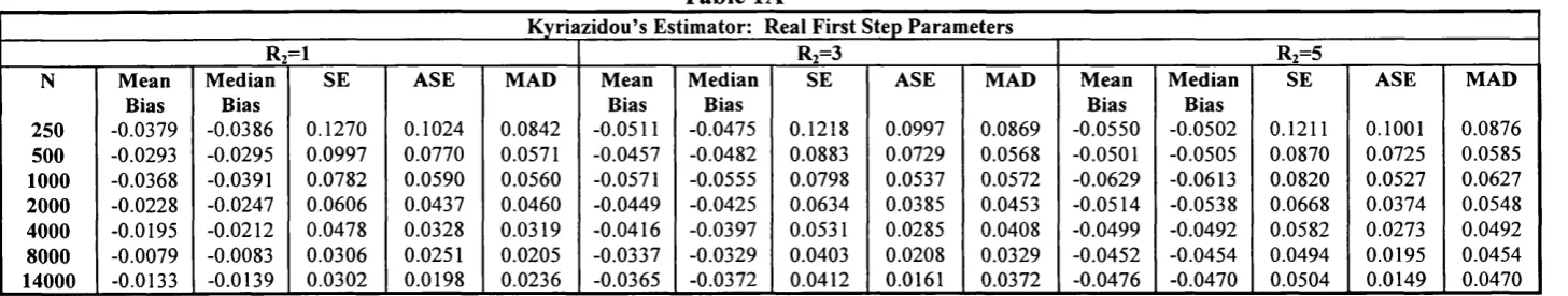
Table 1 presents the finite sample properties o f the two estimators under our

basic Monte Carlo design. The estimates will be consistent since all o f the

assumptions in the methods hold. Going from top to bottom o f Table 1, Table 1A

reports the results for Kyriazidou’s (1997) bias corrected estimator (with 5-^ - 0.9) using the true y in the construction o f the kernel weights. We use a second = 1 ),

® The individual effects design is driven by the fact that w e want to keep both its linear correlation with respect to the explanatory variables, and a normality assumption for its random com ponent. The reason is that W ooldrid ge’s (1 9 9 5 ) estimator assum es normality for the random terms in the selection equation. This means that the difference

betw een 7/, and its conditional mean is a random normal error. At the same tim e, W ooldrid ge’s (1 9 9 5 ) estimator

(42)

TABLE 1: Basic Monte Carlo Design

Table lA

K yriazidou’s Estim ator: Real F irst Step Param eters

Rz=1 Ri=3 Rz=5

N Mean M edian SE ASE MAD Mean M edian SE ASE MAD M ean M edian SE ASE MAD

Bias Bias Bias Bias Bias Bias

250 -0.0379 -0.0386 0.1270 0.1024 0.0842 -0.0511 -0.0475 0.1218 0.0997 0.0869 -0.0550 -0.0502 0.1211 0.1001 0.0876

500 -0.0293 -0.0295 0.0997 0.0770 0.0571 -0.0457 -0.0482 0.0883 0.0729 0.0568 -0.0501 -0.0505 0.0870 0.0725 0.0585

1000 -0.0368 -0.0391 0.0782 0.0590 0.0560 -0.0571 -0.0555 0.0798 0.0537 0.0572 -0.0629 -0.0613 0.0820 0.0527 0.0627

2000 -0.0228 -0.0247 0.0606 0.0437 0.0460 -0.0449 -0.0425 0.0634 0.0385 0.0453 -0.0514 -0.0538 0.0668 0.0374 0.0548

4000 -0.0195 -0.0212 0.0478 0.0328 0.0319 -0.0416 -0.0397 0.0531 0.0285 0.0408 -0.0499 -0.0492 0.0582 0.0273 0.0492

8000 -0.0079 -0.0083 0.0306 0.0251 0.0205 -0.0337 -0.0329 0.0403 0.0208 0.0329 -0.0452 -0.0454 0.0494 0.0195 0.0454

14000 -0.0133 -0.0139 0.0302 0.0198 0.0236 -0.0365 -0.0372 0.0412 0.0161 0.0372 -0.0476 -0.0470 0.0504 0.0149 0.0470

n î

i

K ) S C/D > § S "0

I

S 0 'n H

1

en (/) H 5 O c/o

Table IB K yriazidou’s Estim ator: Estim ated F irst Step P aram eters

R]—1, Ri~3

W ooldridge’s E stim ator

N M ean Bias M edian SE ASE MAD M ean Bias M edian SE ASE MAD

Bias Bias

250 -0.0355 -0.0249 0.1431 0.1067 0.1032 -0.0104 -0.0165 0.1217 0.1275 0.0888

500 -0.0433 -0.0413 0.0945 0.0777 0.0653 0.0123 0.0022 0.0935 0.0897 0.0594

1000 -0.0168 -0.0138 0.0696 0.0583 0.0420 -0.0085 -0.0120 0.0619 0.0637 0.0405

2000 -0.0114 -0.0097 0.0638 0.0446 0.0494 0.0041 0.0007 0.0489 0.0451 0.0333

4000 -0.0127 -0.0098 0.0360 0.0331 0.0283 -0.0048 -0.0061 0.0289 0.0320 0.0210

8000 -0.0086 -0.0146 0.0390 0.0259 0.0297 -0.0007 -0.0004 0.0208 0.0225 0.0156

(43)

a fourth {Rj = 3 ) and a sixth ( R2 = 5 ) order bias-reducing kernel function^. The

bandwidth sequence is respectively. We

chose the initial c equal to 1. Then, we compute p based on and construct

(Sj, defined in section 2 above. We use P and (f,, to compute the estimates o f and as in (2.31), (2.32), and (2.33), respectively. Then we

estimate c* by c , using equation (2.30) with S ^ , and E^^ replaced by their consistent estimates. The asymptotic bias-corrected estimator is computed as in (2.27)

using c as the constant in the definition o f and . On the left-hand side o f Table IB we focus on the case o f a second order bias-reducing kernel function and y

^ We use high {Rj + 1 ) order bias reducing kernels constructed follow ing Bierens (1987). For z j G 93 and [(./?2 + l ) / 2 ] > 1 let

p = \ _{(V 2^)|}_a_{, | V M} _o₎

where Q is a positive definite matrix and the parameters 9 ^ and fJ.^ are such that ^ = 1 and

p = \

(/?z + l)/2

_

= 0, for = l,2,...,[^(i?2 + 0 /^ ] ~ We should specify Q = F, where V is the

p=i

sample variance matrix; that is, V = ( \ l |^(z „ - z - Z j ^(z -, — z ] / - Z with

- 'V

Z = (1/ R2 + ^ = 2,4,6, . . . , w e get

2

p

- r/ N , 1 q i/2 ) [(z „ -z ,,)i> /c „ ]K -'[( z „ - z ,,) j> /c „ ]///

- z , J r A « J = 2 , ---

^---For /?, = 1 w e set ^, = //, = 1 ; for /?2 ~ ^ we set 6 ^ = 2, 6 2 = -1 , //, = 1, and /J. 2 = V 2 ;

(44)

is estimated by the SCMSE. The SCMSE is computed by maximising (2.18) with

respect to given y, =1 by scale normalisation in all o f the Monte Carlo

replications^^. For L we use in (2.19), so i?, +1 = 4 and the optimal rate o f convergence for y is , faster than the rate o f convergence for p The results are those for 5^ = 0.1. The bandwidth parameter for the SCMSE was constructed as follows. Given i ? , +1 = 4, we chose cr^ = and

. We then compute the SCMSE y based on , and use y

and to compute À, D, and C by (2.22), (2.23), and (2.24), respectively. Then we estimate i9* by 5 , where 3 is obtained from 3* in section 2 by replacing A, D,

and C with A, D, and C . For Q the identity matrix was used. Table IB reports on the right-hand side the results for the minimum distance version o f W ooldridge’s

(1995) estimator.

From Table 1 we see that W ooldridge’s (1995) estimator is less biased than

Kyriazidou’s (1997) estimator both with and without estimated first step parameters.

Furthermore, Wooldridge’s (1995) estimator reaches its asymptotic behaviour faster

due to the fact that this estimator is V # -consistent. Kyriazidou’s (1997) estimator is

consistent at a rate slower than and for this reason behaves well for bigger

(45)

sample sizes. For this estimator the more satisfactory results are obtained with the

normal kernel density function ( = 1 )•

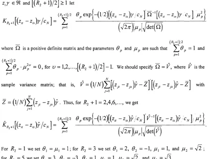
In Table 2 we generate a misspecification problem for W ooldridge’s (1995)

estimator. In Table 2A the linear projection functional form for the individual effects

in the main equation has been violated. We have generated the true a , ' s by adding to our benchmark specification quadratic terms on the x 's :

ccj

= +

Xj2

) / 2 + +

x^2

j / 2 + -\/2 • A^O,l) +1 • (3.2)

Under this design Wooldridge’s (1995) estimator is clearly inconsistent and it suffers

from a misspecification bias problem. The estimator behaves badly in terms o f all the

considered measures. In Table 2B we invalidate the linearity assumption for the

individual effects in the selection equation by adding quadratic terms on the z's :

Vi ~ (^1/1 ^1/2 ) / 2 + (Zjij + ^2,2 ) / 2 + (z,y, + Z,,2 ) / 2 + (Z2,J + ^2/2) ^ 2 + C- — 1. (3.3)

The inconsistency o f the first step parameter estimates hardly influences the bias for

the second step estimates. Experiments for Kyriazidou’s (1997) estimator are not

included in Table 2 because this estimator is robust against any type o f design for the

individual effects in both equations. As the method is based in estimation with time

differences its properties are independent o f the particular shape o f the individual

(46)

CHAPTER 2. FINITE SAMPLE PERFORMANCE OF TW O ESTIM ATORS _{4 5}

TABLE 2: Generating A Misspecification Problem For Wooldridge

Table 2 A

cc^

= +

Xj2

) / 2 + +

x^2

j / 2 + V

2

• A^O,l) + 1

N Mean Bias Median Bias SE ASE MAD

250 0.4336 0.4293 0.4662 0.1691 0.4293

500 0.4645 0.4637 0.4819 0.1212 0.4637

1000 0.4485 0.4426 0.4576 0.0865 0.4426

2000 0.4518 0.4550 0.4567 0.0610 0.4550

4000 0.4539 0.4528 0.4559 0.0434 0.4528

8000 0.4576 0.4610 0.4585 0.0307 0.4610

14000 0.4549 0.4572 0.4556 0.0231 0.4572

Table 2B

7, = (^1/1 + ^1/2 ) / 2 + (Z;,] + ^2/2 ) / 2 + (zf., + zf,2 ) / 2 + (Z;,, + Z2/2 ) / 2 + c,. - 1

250 0.0290 -0.0155 0.3151 0.3198 0.1647

500 0.0235 0.0431 0.2478 0.2257 0.1960

1000 0.0009 0.0101 0.1568 0.1584 0.II54

2000 -0.0060 -0.0122 0.1048 0.II39 0.0813

4000 -0.0015 -0.0027 0.0840 0.0799 0.0608

8000 0.0050 0.0093 0.0519 0.0564 0.0354

(47)

CHAPTER 2. FINITE SAMPLE PERFORMANCE OF TW O ESTIM ATORS 4 6

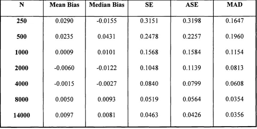
In Table 3 we generate a predetermined variable which affects the set o f

explanatory variables in both equations in (3.1). We invalidate the strict exogeneity

assumption underlying both methods. The predetermined variable = ^2/2 the

new experiment has been generated as

= # ( 0 , l ) + 0.5g„. (3.4)

We report the results for both estimators. Note that the results are very similar when

W ooldridge’s (1995) estimator is used relative to the case where Kyriazidou’s (1997)

estimator is applied. Both estimators show a strong negative bias, and huge SE and

MAD very far from the ASE predicted by the asymptotic theory.

In Tables 4 and 5 we compare Wooldridge (1995) and Kyriazidou’s (1997)

estimators when the conditional exchangeability assumption breaks down. Differently to the baseline design, for Table 4 we have:

~ 0.5 ' #(0,1); w,2 ~ 2 • #(0,1);

c,= 0 .6 -;V (0 ,l);

Kl — ~ ^i\ ’ K2 — “ ^/2 ’

f ,, = 0.8 • #(0,1) + 0.1 • v,i ; = 0.8 • #(0,1) + 0.9 •

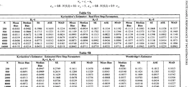
For Table 5 we substitute g,, in (3.5) by = 0.8 • #(0,1) + 0.1 • f,, - 5.

We allow for non-constant variances over time for the error terms and

(48)

CHAPTER 2. FINITE SAMPLE PERFORMANCE OF TW O ESTIM ATORS _{4 7}

TABLE 3: Invalidating Strict Exogeneity

Z2,2 = 77(0,1)+ 0.5^,,

Table 3A: W ooldridge’s Estimator

250 -0.2287 -0.2323 0.2556 0.1138 0.2323

500 -0.2103 -0.2164 0.2289 0.0789 0.2164

1000 -0.2124 -0.2115 0.2197 0.0571 0.2115

2000 -0.2086 -0.2072 0.2129 0.0405 0.2072

4000 -0.2104 -0.2106 0.2130 0.0288 0.2106

8000 -0.2061 -0.2035 0.2071 0.0202 0.2035

14000 -0.2069 -0.2067 0.2076 0.0153 0.2067

Table 3B: Kyriazidou’s Estimator

250 -0.2019 -0.2244 0.2450 0.0990 0.2285

500 -0.2168 -0.2191 0.2322 0.0723 0.2191

1000 -0.2050 -0.2197 0.2150 0.0542 0.2197

2000 -0.2026 -0.2012 0.2089 0.0411 0.2012

4000 -0.2087 -0.2095 0.2127 0.0309 0.2095

8000 -0.1992 -0.2012 0.2011 0.0232 0.2012

(49)

TABLE 4: Invalidating The Exchangeability Assumption In Kyriazidou

~ 0 .5 -A (0 ,l), ~2- A( 0, 1)

c, = 0 .6 -A (0 ,l)

t'/, = - «i,

= 0.8 ■ A(0,1) + 0.1 ■ V , ,, = 0.8 • A(0,1) + 0.9 •

Table 4 A

K yriazidou’s Estim ator: Real First Step P aram eters

Rz=1 R2~3 Rz=5

N M ean M edian SE ASE MAD M ean M edian SE ASE MAD M ean Median SE ASE MAD

Bias Bias Bias Bias Bias Bias

250 -0.0540 -0.0819 0.2057 0.1587 0.1646 -0.0909 -0.0950 0.1984 0.1526 0.1489 -0.1010 -0.1004 0.1963 0.1526 0.1468

500 -0.0584 -0.0705 0.1621 0.1199 0.1158 -0.0979 -0.1047 0.1533 0.1118 0.1196 -0.1091 -0.1148 0.1569 0.1107 0.1231

1000 -0.0672 -0.0847 0.1450 0.0926 0.1078 -0.1133 -0.1188 0.1485 0.0839 0.1188 -0.1285 -0.1339 0.1549 0.0818 0.1339

2000 -0.0399 -0.0508 0.0983 0.0696 0.0781 -0.0917 -0.0949 0.1143 0.0598 0.0949 -0.1094 -0.1087 0.1261 0.0576 0.1087

4000 -0.0447 -0.0416 0.0875 0.0510 0.0574 -0.0888 -0.0906 0.1031 0.0436 0.0906 -0.1091 -0.1122 0.1180 0.0414 0.1122

8000 -0.0196 -0.0115 0.0530 0.0403 0.0378 -0.0727 -0.0713 0.0811 0.0322 0.0713 -0.0963 -0.0965 0.1009 0.0298 0.0965

14000 -0.0157 -0.0188 0.0461 0.0322 0.0325 -0.0661 -0.0640 0.0730 0.0253 0.0640 -0.0933 -0.0913 0.0971 0.0229 0.0913

0

"T3 W

I

s c/5 >

I

0 Ti

1

m c/5

i

O Table 4B K yriazidou’s Estim ator: Estim ated F irst Step P aram eters

R^—1, R i—3

W ooldridge’s Estim ator

N M ean Bias M edian

Bias

SE ASE MAD Mean Bias M edian

Bias

SE ASE MAD

250 -0.0991 -0.1099 0.2636 0.1656 0.1553 -0.0113 -0.0160 0.1444 0.1575 0.0797

500 -0.0770 -0.0761 0.2179 0.1275 0.1180 0.0151 0.0026 0.1201 0.1108 0.0852

1000 -0.0387 -0.0657 0.1706 0.0926 0.0930 -0.0010 -0.0124 0.0802 0.0785 0.0598

2000 -0.0587 -0.0604 0.1076 0.0675 0.0788 0.0018 0.0033 0.0585 0.0557 0.0439

4000 -0.0227 -0.0205 0.0776 0.0537 0.0672 -0.0070 -0.0062 0.0348 0.0392 0.0219

8000 -0.0146 -0.0192 0.0566 0.0412 0.0454 -0.0023 -0.0055 0.0251 0.0276 0.0163

14000 -0.0156 -0.0135 0.0463 0.0328 0.0331 0.0026 -0.0013 0.0232 0.0209 0.0177