University of South Carolina
Scholar Commons
Theses and Dissertations
1-1-2011
3-D Computational Investigation of Viscoelastic
Biofilms using GPUs
Paisa Seeluangsawat
University of South Carolina - Columbia
Follow this and additional works at:https://scholarcommons.sc.edu/etd Part of theMathematics Commons
This Open Access Dissertation is brought to you by Scholar Commons. It has been accepted for inclusion in Theses and Dissertations by an authorized administrator of Scholar Commons. For more information, please [email protected].
Recommended Citation
Seeluangsawat, P.(2011).3-D Computational Investigation of Viscoelastic Biofilms using GPUs.(Doctoral dissertation). Retrieved from
3-DCOMPUTATIONAL INVESTIGATION OF VISCOELASTIC BIOFILMS USINGGPUS
By
Paisa Seeluangsawat
Bachelor of Science
Massachusetts Institute of Technology 2002 Master of Science
University of North Texas 2006
Submitted in Partial Fulfillment of the Requirements
for the Degree of Doctor of Philosphy in
Mathematics
College of Arts and Sciences
University of South Carolina
2011
Accepted by:
Qi Wang, Major Professor
Peter Binev, Committee Member
Hong Wang, Committee Member
Xiaofeng Yang, Committee Member
Guiren Wang, Committee Member
c
Copyright by Paisa Seeluangsawat, 2011
D
EDICATION
A
CKNOWLEDGMENTS
I would like to express my deepest gratitude to my adviser Dr. Qi Wang, who has
guided me through the transition from classroom to research. He is always available for
discussion and regularly provides insights that turn a hard problem into a manageable one.
Without his patient support, this work would be impossible.
I also would like to thank Dr. Hong Wang, Dr. Peter Binev, Dr. Xiaofeng Yang, and
Dr. Guiren Wang for volunteering their time to be on my Dissertation Committee. Several
of them have also taught me tools and theorems that I use in this research.
I am indebted to all my teachers, both at USC and from prior. Their collective
knowl-edge and valuable advices play an integral role in shaping me into who I am.
I appreciate friendships from USC Math faculty, fellow graduate students, and the staff.
Together, they provide a home away from home, and help keep me sane through the ups
and downs of my graduate school life.
Last but not the least, I would like to thank Xiao Xiao for taking care of me when I do
A
BSTRACT
A biofilm is a slimy colony of bacteria and the materials they secrete, collectively called
“extracellular polymeric substances (EPS)”. The EPS consists mostly of bio-polymers,
which cross link into a network that behave viscoelastically under deformation. We
pro-pose a single-fluid multi-component phase field model of biofilms that captures this
be-havior, then use numerical simulations on GPUs to investigate the biofilm’s growth and its
hydrodynamics properties.
We model a biofilm immersed in a solution as a two-phase fluid, consisting of the
solution, which is modeled as a viscous fluid, and the biomass, which is modeled as a
viscoelastic solution with viscosity much higher than that of the solution. Each fluid has its
own velocity field, but the important quantity is their combined volume-averaged velocity,
which is the main physically observable quantity. The theory is developed with this average
velocity in mind, while tracking the individual velocities using the excessive velocity of
each fluid, which is calculated from the given mixing free energy density.
By using the phase field model, the whole domain is governed by a single set of
govern-ing equations, simplifygovern-ing the numerical procedure significantly. The model accounts for
Cahn-Hilliard phase mixing and nucleation, biomass growth from nutrient consumption,
nutrient diffusion, fluid flow interaction, viscous stress due to bacteria and the solution,
and elastic stress due to the EPS.
We use a finite difference scheme based on a staggered grid in 2-D and 3-D
geome-try. The incompressible Navier-Stokes equation is solved by the Gauge-Uzawa method,
modified so that it can be quickly solved using Fast Fourier Transform (FFT). The elastic
region, which we solve by a backward interpolation and an explicit updating scheme. The
remaining equations are discretized using a semi-explicit scheme and solved iteratively by
the BiCG-stab method.
The numerical scheme is implemented on graphics processing units (GPUs), which
offers up to a hundred fold speed up over a traditional single-thread CPU. Our numerical
implementation is carried out such that only a small amount of key parameters are passed
between CPU and GPU, while large data are kept in GPU at all time in order to avoid the
relatively low bandwidth and high latency of the CPU-GPU data transfer. They are copied
to the CPU memory only occasionally in order to output to a file. Data are laid out in
the GPU memory in such a way that GPU threads can fetch them in a coalesced manner
to increase the speed of data access. We use the CUFFT package for the fast Fourier
transform, and the Thrust and CUSP libraries for BiCG-stab and data management.
We carry out numerical simulations in both two and three spatial dimensions. The
vis-coelastic results are compared with those from the viscous model at two distinct timescales
relevant to biomass growth and an imposed shear flow. In the growth timescale,
mea-sured in days, which is much longer than the elastic relaxation time, both models predict
nearly identical results. This is simply because the viscoelastic model behaves like a
vis-cous model since the elastic relaxation time is so short that the elastic effect is not felt
strongly at this time scale. In the shear timescale, measured in seconds, which is shorter
than the elastic relaxation time, the viscoelastic model predicts biofilms that deform under
shear more than those predicted by the viscous model. In 3-D, the viscoelastic model
pre-dicts that a portion of the biomass can be pulled into a nose shaped and stream along with
the flow. After the external shear ceases, the viscoelastic model predicts that the biofilms
partially recoil back toward their original position, while the viscous model predicts that
the biofilms stop moving. Nutrient distribution and its effect to biofilm growth is
investi-gated by the numerical solver revealing inherent hydrodynamic interaction in the material’s
pro-vide a valuable predicative tool for biofilm research, in particular, for the investigation of
C
ONTENTS
DEDICATION . . . iii
ACKNOWLEDGMENTS . . . iv
ABSTRACT . . . v
LIST OFTABLES . . . x
LIST OFFIGURES . . . xi
CHAPTER 1 INTRODUCTION . . . 1
1.1 Biofilm . . . 1
1.2 Biofilm models . . . 6
1.3 Viscoelastic models . . . 11
CHAPTER 2 BIOFILM MODEL . . . 16
2.1 Constitutive equations . . . 17
2.2 Nondimensionalization . . . 20
2.3 Remark about the stress constitutive equation . . . 22
CHAPTER 3 NUMERICAL SCHEMES AND GPUIMPLEMENTATION . . . 24
3.1 Numerical scheme . . . 24
3.2 Momentum equation . . . 30
3.3 Elastic stress equation . . . 46
3.4 Biomass volume fraction equation . . . 47
3.6 Mesh refinement . . . 60
3.7 Visualizing a stress field . . . 69
CHAPTER 4 NUMERICAL SIMULATION AND DISCUSSIONS . . . 71
4.1 Growth dynamics of biofilms . . . 73
4.2 Biofilm dynamics in shear flows . . . 76
CHAPTER 5 CONCLUSION . . . 94
BIBLIOGRAPHY . . . 96
APPENDIXA SOLVING THEHELMHOLTZ EQUATION BYDFT . . . 103
A.1 One dimension . . . 104
A.2 Two and three dimensions . . . 109
A.3 Verification . . . 110
APPENDIXB GRID REFINEMENT ANALYSIS . . . 112
B.1 Convergence rate . . . 112
B.2 Global Error . . . 113
L
IST OF
T
ABLES
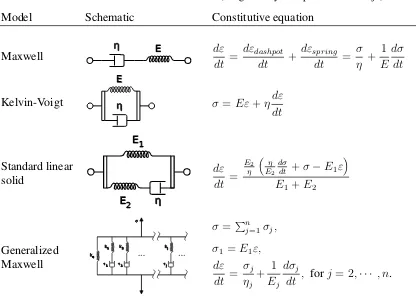
Table 1.1 Linear viscoelastic models . . . 12
Table 3.1 Decay rate of then+ 1−interpolation scheme . . . 39
Table 3.2 2-D spatial refinement result for growing a biofilm with∆t = 10−4 . . . 63
Table 3.3 2-D temporal refinement result for growing a biofilm with∆x= 1/1024 64
Table 3.4 3-D spatial refinement result for growing a biofilm with∆t = 10−4 . . . 65
Table 3.5 3-D temporal refinement result for growing a biofilm with∆x= 1/240 . 66
Table 3.6 2-D spatial refinement result for shearing a biofilm with∆t= 10−5 . . . 67
Table 3.7 2-D temporal refinement result for growing a biofilm with∆x= 1/1024 67
Table 3.8 3-D spatial refinement result for shearing a biofilm with∆t= 10−5 . . . 68
Table 3.9 3-D temporal refinement result for growing a biofilm with∆x= 1/240 . 68
Table 4.1 Parameter values used in the simulations . . . 72
Table A.1 Spatial refinement of the Navier-Stokes solver . . . 111
L
IST OF
F
IGURES
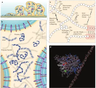
Figure 1.1 Biofilm developmental stages. . . 2
Figure 1.2 Model of biofilm EPS. . . 2
Figure 1.3 Cell specialization within a biofilm colony. . . 4
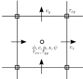
Figure 3.1 Variable locations on the 2-D staggered grid . . . 27
Figure 3.2 Solution of Eq.(3.81). The real part of eachλis plotted as a function ofc. . . 40
Figure 3.3 The incorrect assumtion that vy=1 = 0 can introduce a boundary error of order10−7 on each time step . . . 45
Figure 3.4 Shear profile for 1-D flow in a 2-D domain. . . 45
Figure 3.5 The bulk free energyf˜and its second derivative . . . 49
Figure 3.6 Inflection pointsφ1, φ2 of the bulk free energyf˜(φn). The biomass nucleates whenφn∈(φ1, φ2). . . 50
Figure 3.7 2-D mesh refinement of growing a biofilm. Profiles att= 0andt = 2. . 63
Figure 3.8 3-D mesh refinement of growing a biofilm. Profiles att= 0andt = 2. . 65
Figure 3.9 2-D mesh refinement of shearing a biofilm. Profiles att= 0andt= 2. . 67
Figure 3.10 3-D mesh refinement of shearing a biofilm. Profiles att= 0andt= 2. . 68
Figure 4.1 Initial biomass volume fractionφnprofile. . . 79
Figure 4.2 Biomass volume fractionφn, nutrient concentrationc, nutrient con-sumption rategc, and biomass production rate gn in the simulation of a growing bud of biofilm att = 300 . . . 80
Figure 4.3 Velocityv, biomass fluxφnvn, and pressurep . . . 81
Figure 4.5 Snapshots of the simulation of a growing randomly scattered bits of
biofilm . . . 83
Figure 4.6 The left and right colonies grow faster than those in the middle. . . 84
Figure 4.7 Biomass flux, elastic stress, and viscous stress due to bacteria . . . 85
Figure 4.8 Net forces in a growing colony of biofilm. . . 86
Figure 4.9 Growing a bud of biofilms in 3-D . . . 87
Figure 4.10 Snapshots of growing scattered bits of biofilms in 3-D . . . 87
Figure 4.11 Biomass volume fractionφn, average velocityv, and pressurep . . . 88
Figure 4.12 Elastic stress and viscous stress distributions . . . 88
Figure 4.13 Forces in the momentum equation . . . 89
Figure 4.14 Shearing the biofilm grown from a small bud . . . 89
Figure 4.15 Shearing of a 3-D biofilm grown from a bud . . . 90
Figure 4.16 Shearing of a 3-D biofilm grown from scattered bits . . . 91
Figure 4.17 Shearing of a 3-D colony of biofilm with fewer buds . . . 92
Figure 4.18 Shearing an biofilm lump with a thin neck. The biofilm colony de-taches at high shear rates. . . 93
C
HAPTER
1
I
NTRODUCTION
1.1 BIOFILM
Biofilms are the slimy materials commonly found on moist surfaces. They are
ubiqui-tously found on plants and in river beds, kitchen sinks, water pipes, water filters, medical
implants, in body tissues, to name a few. A biofilm is a mixture of bacteria, the slimy
materials they produced, which are made up of polysaccharides, proteins, and other
bio-materials collectively called “extracellular polymeric substances” (EPS), and water. The
EPS harbors bacteria from surrounding environments, allowing them to communicate via
chemical signals and cooperate their self-defense against harsh chemicals. Many biofilms
are cooperative ecosystems of several species of bacteria, as well as fungi, algae, yeasts,
protozoa, and other microorganisms.
More information about biofilm can be found in the review articles [20] [11] [45].
We give a brief overview here. Figure.1.1 illustrates developmental stages of a biofilm
colony. Planktonic cells first attach to a surface, also called substratum. They then start
producing EPS and multiply their quantity. The biofilm colony grows as cells multiply
and more EPS are produced. Once matured, the colony releases planktonic cells, which
disperse on new substrate to form a new colony. Each stage in the figure is accompanied
by a photomicrograph of Pseudomonas aeruginosa, a model organism for biofilm study
[20] [74]. Biofilms can form layers with thickness that ranges from a few microns to a few
centimeters.
dis-Figure 1.1: Left: Biofilm developmental stages. Each stage is illustrated by a drawing (top) and a photo of a P. aeruginosa biofilm (bottom). (1) Planktonic cells land. (2) Cells irreversibly attach to the site. (3) Cells start secreting EPS. (4) The biofilm grows into a mature colony. (5) Some cells disperse back into the solution. (Figure by D. Davies in [62] [40]) Right: a scanning electron micrograph (SEM) of P. aeruginosa(by Janice Haney Carr, Centers for Disease Control and Prevention).
tinctive phases [71] [66],
1. Lag phase. Organism undergoes phenotypic change to adapt to the environment and
produces necessary RNA and enzymes to get ready for cell division.
2. Exponential phase (also known as logarithmic phase). Cells multiplies (a.k.a.
di-vide), causing exponential growth. The growth rate depends on the species and
en-vironment. For example, the doubling time of P. aeruginosa is about 20 minutes in
mice lung [59] and 100 minutes in human lung [73]. On the other hand, T. pallidum
in rabbit testes takes about 30 hours to double [42].
3. Stationary phase. Nutrient starts to be scarce, and waste products accumulate. The
growth slows down, and is balanced out by the death rate.
4. Death phase. Nutrient diminishes.
Aside from lack of nutrient, cells can also die from drugs and harsh chemical
treat-ments. However, drugs do not affect all cells equally. Even within the same species, some
cells are more resistant to drugs than others. These are known as persistors. They neither
grow nor die in the presence of a specific drug. When the drug subsides, these persistors
divide again. However the rejuvenated colony does not inherit this persistence. They still
show the same level of susceptibility to the same drug [4] [37].
Inside the biofilm, cells are tangled inside the EPS network, greatly reducing their
mobility. This allows chemical gradient to develop, thus encourages cells inside biofilm
to specialize in different functions and benefit from each other. In an example from [67]
(Fig.1.3), cells on the EPS-solution interface specialize in efflux pump, which keep drug
out of the EPS while allowing nutrient to pass, while younger cells divide and grow in the
interior.
Several experiments study the hydrodynamics properties of biofilms [63] [61] [32] [56].
ding), rolling, and viscoelastic recoil. Outside labs, biofilms have been studied in its natural
habitat such as river sediments [21] and rocks under river falls [29].
Key parameters of viscoelastic materials are the elastic modulus and relaxation time.
There is a wide range of the biofilm elastic shear modulus, from 10−2 to 105 Pa [57].
The value depends on the species of bacteria. Even within the same species, different
papers report values that differ by 1-2 order of magnitudes. This is partly because the
biofilm is a live heterogeneous material, thus its elasticity differs from specimen to
speci-men. Furthermore, chemical compositions of the environment can alter the strength of the
EPS [34]. Additionally, some discrepancy is attributed to the different measurement
meth-ods and the difficulties in interpreting the experimental results [1]. The relaxation time of
various species of biofilms are reported to be about 18 minutes [57]. However, a newer
measurement technique using a microfluidic device come up with the relaxation time of S.
epidermidis at 14 seconds [26]. This could be because a biofilm has multiple relaxation
times.
Biofilms can cause many industrial problems. They corrode surfaces, clog pipes,
in-crease fluid drag, and reduce heat transfer. They make surfaces harder to clean and
disin-fect, posing important risks in food processing and medical settings. Inside human body,
biofilms shield pathogens from antibiotics and the host’s immune system. Rather than
sparsely spreading out throughout the body, bacteria cooperate and thrive together inside
a biofilm. Detachment process allows a group of pathogens to migrate to a new location
together [24]. On the positive side, biofilms can be harnessed to some industrial benefits in
waste treatment, bio-barrier, and microbial fuel cells. A better understanding of biofilms
will not only provide scientific insights into the intriguing biomaterial system but also make
1.2 BIOFILM MODELS
It is a challenge to model the live microorganism in biofilms and their transient growth
and transport behavior. There have been many mathematical models for studying biofilms,
some dating back to early 1980’s. They differ in the phenomena of interest, key variables,
physical effect considered, and numerical methods. Recent reviews of these models include
[48], [16] [33] and [68].
The most commonly studied phenomena are growth at the expense of nutrient
con-sumption, and biomass movement. Other phenomena of interest are cell death, quorum
sensing, and phenotypic shift. These phenomena occur on different timescales,
• seconds: advection, diffusion, cell motility
• minutes: elasticity
• hours: phenotypic shift, cell division, nutrient consumption, death by drug
• days: colony growth, death by starvation
The set of phenomena we desire to capture partially dictates the list of key quantities that
we need to keep track of. The most common ones are representations of biomass, nutrient,
and their hydrodynamics. Other quantities include drug, signaling chemical, phenotypic
ratio, and elastic stress.
Biomass
A modeler may choose to keep track of the biomass as a single material entity [52] [13]
[27] [47], or separate them into two separate materials of distinct material’s properties:
bacteria and EPS parts [38]. More sophisticated models may keep track of several species
or several phenotypes of a specie [69] [51] [46]. Models differ in how these quantity
are represented. For example, the location and amount of biofilms in water have been
• Location of biofilm-water interface [54] [69] [13]
• Cellular automata on a lattice [52] [28] [51]
• Individual bacteria in the continuum [35] [46]
• Scalar field of biofilm concentration [13] [17] [75] [76] [47]
A hybrid approach [50] [49] [47] is to represent the biomass as a concentration field, but
once the concentration reaches a threshold, the biomass spreads to adjacent cells using
cellular automation algorithm.
Nutrients, drugs, and other chemicals
While a biofilm growth might require several types of nutrient, it is typical to have one
nutrient that is the most essential, thus predominantly determines the enzymatic reaction
rate. Many numerical simulations pick this rate-limiting nutrient to be dissolved oxygen
(DO) [50] [49] [27] [47]. However, some models use a different rate-limiting nutrient such
as glucose [28]. Some models keep track of multiple nutrients [69] [35] [41] [46].
In addition to nutrient, some models incorporate drugs or harsh chemicals which inhibit
growth, kill bacteria, or erode the EPS [38]. Some allow bacteria to produce waste products
which might hamper growth or become a nutrient for other species [46]. Others yet include
a chemical signal that bacteria release as a part of quorum sensing. We will refer to these
components collectively as chemicals.
Chemicals are usually modeled as a scalar field of concentration, along with Fick’s
laws of diffusion [69] [50] [49] [13] [17] [52] [47]. For low nutrient concentration, an
alternative approach is to apply a diffusion-limited aggregation model [72] [65] [51], in
which each individual nutrient molecule does a random walk until it hits a biofilm and gets
consumed. This tends to produce biofilms that grow into fractal-like branches instead of a
In models where biomass and solutions can mix, there are two approaches in keeping
track of the chemicals,
• Chemicals exist in both biomass and solution. With the chemical concentrationcper
volume and diffusion constantDs, the diffusion equation is ∂c∂t =Ds∇2c.
• Chemicals exist only in the solution. If a chemical has dissolved concentration c
inside the solution of volume fractionφs, then its spatial concentration is cφs. The
appropriate diffusion equation is ∂cφs
∂t =∇ ·Dsφs(∇c).
Note thatDscan be modeled as a constant, or a function of concentrationscandφs.
The source of chemicals can also be modeled differently,
• Fixed concentration at the domain boundary [13] [17] [35] [41] [75] [76]. Thus
nutrient reaches the biomass by advection and diffusion.
• Fixed concentration at the biofilm-solution interface [69] [41]. This follows from the
assumption that the solution is well-mixed outside the biomass.
• Fixed concentration at the top biofilm height [46].
• Flux balance at the biofilm-solution interface [69], [52]. LetDbulk andDbiof ilm be
the diffusion constants in the bulk fluid and inside biofilm respectively. LetLbe the
width of diffusion layer. This condition is imposed at the interface,
Dbulk(cbulk−cinterf ace)/L=Dbiof ilm
∂c ∂x
interf ace
. (1.1)
• Fixed concentration in the inflow solution [53] [47].
• Fixed boundary flux [51].
• Chemicals produced inside the domain.
The choice of chemical sources partially determines the handling of boundary conditions.
• Impermeable (zero flux:~n· ∇c= 0).
• Permeable. The boundary condition depends on specific settings.
• Reactive (c= 0).
Rate of growth/consumption
The rates of biofilm growth and nutrient consumption are often modeled by the Monod
equationrate = ratemaxc
K+c , wherecis the nutrient concentration,ratemax is the maximum
consumption rate that can be a function of bacterial concentration, and K is a constant
known as the half saturation constant. The Monod model gives a nearly linear consumption
rate at small c and becomes independent ofcas it is large. Note that Monod equation looks
exactly the same as Michaelis-Menten equation, thus hinting that enzyme kinetics underlies
the growth and consumption process.
If the biomass is represented by cellular automata, growth usually means increasing
the number of automata, representing cell division [52] [51]. If the model keeps track
of individual bacteria, each cell can grow in volume, shoving its neighbors aside, and
split into two smaller cells [35] [46]. If biomass is demarcated by biofilm-water interface,
growth is represented by increased biomass volume. The interface location can be directly
modified to account for additional volume [69]. Alternatively, the growth can modify local
pressure, which drives a flow that eventually expands the biomass volume [13]. If the
biomass is represented by a concentration field, growth can be represented by an increase
in concentration. In such model, one still needs a mechanism for the biomass to spread out
to neighboring regions. Otherwise, the regions that start off without biomass will continue
to have no biomass. This spreading can be done by ad-hoc diffusion [17], Cahn-Hilliard
dynamics [75] [76], or cellular automata rule [50] [49] [47].
Models can also account for death of bacteria, modeled as an ad-hoc decay [52] [51]
Hydrodynamics
Some models consider biofilm growth in static medium [69] [50] [49] [52] [51]. Such
models consider diffusion, but often ignore advection. When advection is considered, the
velocity field can be described by,
• One velocity field which convects everything [13].
• One velocity field for water. Biomass is assumed to be stationary [17].
• Separate velocity fields for water and biofilm [9] [10].
• One mass-averaged velocity field, together with excessive velocitiesvwater−vaverage
andvbiof ilm−vaverage [75] [76] [38].
The velocity field is usually modeled by Darcy’s law [13] or the incompressible
Navier-Stokes equation [75] [76].
Other features
In many models, one can find an analytic solution or partial solution in one
dimen-sion. Higher spatial dimensions usually require numerical simulations. The advantage of
modeling in two spatial dimensions or higher lies in the ability to model heterogeneous
biofilm-solution surface. More importantly, it is close to the "real thing". Some
phenom-ena like channel flow requires a 3-D simulation. On the other hand, modeling in higher
dimensions incurs significantly more computational overhead.
Most simulations are done on a rectangular domain due to its simplicity. Some
simula-tions were carried out on more complicated domain using the finite element method [47].
Some authors incorporate a user interface so that their program can be used by other
1.3 VISCOELASTIC MODELS
There are many in-depth books on viscoelasticity, which sits at the intersection of
rhe-ology, polymer physics, and mechanical engineering, and chemical engineering. We give
a very brief overview here. For further details, please consult [5], [3], [8], [25]. Physical
theories behind these constitutive models are discussed in [15] and [14].
Viscosity is a generalization of friction. When two flat surfaces rub against each other
at a constant normal force, it experiences a friction forceF =−const v. Both friction and
viscosity convert kinetic energy into heat. Elasticity is epitomized by a spring. When one
pulls a spring by a distancexaway from the equilibrium, one experiences an elastic force
F =−const x. Elastic force converts kinetic energy to potential energy.
Viscoelastic materials exhibit both viscous and elastic behavior. Kinetic energy is
con-verted partly to potential energy and partly to heat. There are many viscoelastic models. In
1-D, the key variables are stressσand strainε. For linear models, the elastic component is
represented by a spring with constitutive equationσ =EεwhereEis the elastic modulus.
The viscous component is represented by a dashpot with constitutive equationσ=ηdεdt.
Dashpot and spring can be combined to form a viscoelastic model in several ways, as
shown in Table.1.1. Maxwell model accurately describes stress relaxation, while
Kelvin-Voigt better describes creep flows. Other models combined more dashpots and springs to
improve models’ accuracy, at the cost of increased parameters and mathematical
complex-ity. Linear models are suitable for small strain. At larger strain, materials can exhibit
non-linear damping or fracture. Alternatively, one can start with thegeneral linear viscoelastic
model
σ(t) =
Z t
−∞G(t−t 0
) ˙ε(t0)dt0 (1.2)
whereε˙ = dεdt andG: [0,∞) → Ris called the relaxation modulus. WhenG(t) =ηδ(t)
where δ is the Dirac delta function, we get a viscous fluid σ = ηε˙. When G(t) = E is
Table 1.1: Linear viscoelastic models(Diagrams by Wikipedia user Pekaje)
Model Schematic Constitutive equation
Maxwell E dε
dt = dεdashpot dt + dεspring dt = σ η + 1 E dσ dt Kelvin-Voigt E
σ=Eε+ηdε dt Standard linear solid E1 E2 dε dt = E2 η η E2 dσ
dt +σ−E1ε
E1+E2
Generalized
Maxwell 1 2 j
k1 k2 kj
ke
σ=Pn
j=1σj,
σ1 =E1ε, dε dt = σj ηj + 1 Ej dσj
dt , forj = 2,· · · , n.
generally want the stress to be affected mostly by recent shear history. Thus we setG(t)to
be a decreasing function tending to zero, for exampleG(t) = Ee−t/λ.
Convected derivatives
Before we generalize these viscoelastic models into higher spatial dimensions, we first
have to learn aboutcodeformational derivatives. Recall that, for any scalar fieldφ, the time
derivative ∂φ∂t in material frame can be converted into the Eulerian frame as the material
derivative DφDt := ∂φ∂t +v· ∇φ. The extra term originates from the change in material’s
location due to the flow fieldv. In addition to this, the flow field also rotates and bends
the basis of the tensor. Scalar quantities don’t feel this, but tensor quantities do. Given
a basis that convects, rotates, and deforms along with the flow, the time derivative of a
the upper convected time derivative,
∇
τ:= Dτ
Dt −(∇v)·τ−τ ·(∇v)
T. (1.3)
Here(∇v)ij := ddxvi
j. Some books define(∇v)ij differently as ∂ivj, thus gives
∇
τ= DτDt −
(∇v)T ·τ −τ·(∇v).
The time derivative of a second order covariant tensor τij in that frame translates into
Eulerian frame as the lower convected time derivative,
∆ τ:= Dτ
Dt + (∇v)
T ·τ+τ·(∇v). (1.4)
Alternatively, one can think ofτ∆as the time derivative of a contravariant tensor in a frame
whosedual basisdeforms along with the flow.
We now define the Gordon-Schowalter convected derivative. This has one parameter
0≤ξ≤1called slippage. Equivalently, some literature usea= 1−2ξ, thus−1≤a≤1.
τ := dτ dt :=
Dτ Dt +ξ
∇
τ +(1−ξ)τ ,∆ (1.5)
= Dτ
Dt −(∇v)·τ−τ ·(∇v)
T +ξ(D·τ +τ·D), (1.6)
= Dτ
Dt −W·τ +τ·W−a(D·τ +τ·D), (1.7)
whereDandWare the rate-of-strain tensor and the vorticity tensor respectively,
D = 1
2[∇v+∇v
T], W= 1
2[∇v− ∇v
T].
(1.8)
Whenξ = 0(a = 1) we recover τ∇. When ξ = 1 (a = −1) we recover ∆τ. Whenξ = 12
(a= 0) we haveτ= DτDt−W·τ+τ·W, which is called co-rotational derivative or Jaumann
derivative. It is the time-invariant derivative for second order tensors. This arises when the
basis rotates but does not deform along with the flow. By comparing (1.6) to (1.3), we can
see thatτis equivalent to taking the upper convected derivative under the effective velocity
gradient∇v−ξD.
For quantitiesφthat have unit “per volume”, the material derivative is DφDt +v· ∇φ=
∂φ
∂t+v·∇φ+φ∇·v= ∂φ
∂t+∇·(vφ). Thus one often sees the term∇·(vφ)instead ofv·∇φ
Going from 1-D to 3-D
Imagine an infinitesimal cube of fluid, surrounded by fluid of the same type. As fluid
flows, neighboring fluid exerts forces on each face of the cube. This force is proportional
to surface area: dF = τ ·ndS, wherenis the unit external normal and dS is the surface
element. The quantity τ is called stress, which is a second order tensor. The angular
momentum balance implies thatτ is a symmetric tensor. Divergence theorem yields the
force on the cubedF= (∇ ·τ)dV. In continuum mechanics, the word “force” usually is a
shorthand for force density per volumef := dF
dV =∇ ·τ.
The simplest model of liquid, known as incompressible Newtonian fluid, stipulates that
τ = 2ηD, whereD = 12(∇v+∇vT)is the rate-of-strain tensor andηis the fluid’s viscosity.
Assuming homogeneity in the viscosity η = const, and using of the incompressibility
condition∇ ·v= 0, one can work out the viscous force,
f =∇ ·τ =η∇2v+η∇(∇ ·v) = η∇2v
(1.9)
The Maxwell constitutive equation from Table.1.1 can be rewritten asσ+λdσ dt =η
dε dt,
where λ = Eη is the relaxation time. This generalizes into higher spatial dimensions as
the upper convected Maxwell (UCM) model when we replace the time derivative by the
convective derivative for second order tensors
τ +λτ∇= 2ηD, (1.10)
which is the key ingredient for several viscoelastic models. The commonly used single
relaxation time constitutive equation models are given below [5].
• Johnson-Segalman,
τ +λ τ= 2ηD (1.11)
• Giesekus,
αλ η τ
2+τ +λ τ∇= 2ηD, (1.12)
• Phan-Thien-Tanner,
αλ
η tr(τ)τ +τ +λ
∇
τ = 2ηD linear form (1.13)
τexp(αλ
η tr(τ)) +λ
∇
τ = 2ηD exponential form (1.14)
• White-Metzner
τ +λI2
∇
τ= 2ηI2D (1.15)
where I2 = 12(D : D −tr(D)2) is the second invariant of D. Incompressibility
yieldstr(D) = 0, henceI2 = 12D:D = 12Pi
P
jD2ij.
When Gordon-Schowalter derivative is used, the slippage parameterais usually set close
to1, that isτ≈τ∇. It is justified physically by assuming some slippage in the microscopic
network, causing them to travel at a different velocity thanvbut not far away from it.
If we assume that the total stress is a combination of UCM and Newtonian stress, we
haveτ =τn+τps whereτn+λ1
∇
τ= 2ηnDandτps = 2ηpsD. Then,
τ +λ1
∇
τ = 2(ηn+ηps)D+ 2λ1ηps ∇
D (1.16)
Letη=ηn+ηps be the total viscosity. Letλ2 =λ1ηnη+psηps be the retardation time [5]. We
have,
τ+λ1
∇
τ = 2η(D+λ2
∇
D). (1.17)
This is known as convected Jeffreys model or Oldroyd’s fluid type B. Since ηn and ηps
are nonnegative, we have0 ≤ λ2 < λ1. We recover the UCM model when λ2 = 0and
Newtonian model whenλ2 =λ1.
Let I be the identity. Notice that I= 2aD. We define the conformation tensor c =
τ +aλη I. Then the Johnson-Segalman model can be rewritten as,
c+λ c= η
aλI. (1.18)
Notice that ifcis initially nonnegative definite, then it will stay nonnegative definite. This
reformulation of the Johnson-Segalman model will be exploited to design our numerical
C
HAPTER
2
B
IOFILM MODEL
We model biofilms using a phase-field based hydrodynamic theory formulation, in
which the EPS production and nutrient consumption are effectively accounted for. We treat
the biofilm and the ambient fluid as a unified mixture system, in which the biomass,
con-sisted of the bacteria and EPS, is modeled collectively as the polymer solution phase; and
the other components, mainly solvent and nutrients, are effectively modeled as an effective
solvent phase. The effective solvent is modeled by a Newtonian fluid which is governed by
the incompressible Navier-Stokes equation.
The volume inside the mixture domain is divided into two components, the biomass
and the solution. A scalar field is introduced to keep track of their volume fraction at
each point in the domain. In the pure solvent region in the ambient fluid, the volume
fraction of the biomass vanishes. Each component has its own velocity field. However,
the boundary condition for each individual volocity field is hard to define and physically
measure. To circumvent this, we use a single fluid model, in which a single mass averaged
velocity serves as the only measurable macroscopic velocity while the individual velocities
are calculated from the intermixing fluxes.
Zhang, Cogan, and Wang [75] [76] have developed, analyzed and simulated such a
model in 1-D and 2-D viscous settings. Here, we extend this model to include elastic effect
2.1 CONSTITUTIVE EQUATIONS
We model biofilms growing inside a tank of liquid solution. The scalar fieldφndenotes
the volume fraction of the biomass, which includes bacteria and EPS. Letφs denote the
volume fraction of the liquid solution. We haveφn+φs = 1, thus only one of the volume
fractions needs to be tracked. Let cdenote the nutrient concentration level, which floats
only inside the solution. Thus, its density per volume iscφs.
Letvbe the average velocity, andpbe the hydrostatic pressure. The phase field theory
for biofilms consists of four sets of equations.
Momentum and continuity equation
ρDv
Dt =∇ ·(aτn+φnτps+φsτs)−[∇p+γ1kBT∇ ·(∇φn∇φn)],
∇ ·v= 0.
(2.1)
Here, ρ = φnρn +φsρs is the effective material density for the fluid mixture, where ρn
andρsare the densities for the biomass and the solvent respectively. The extra stress in the
solvent isφsτs. In the biomass, there is a viscoelastic stressaτn due to the EPS polymer
network and a viscous stressφnτpsdue to the bacteria. The constantais the slip coefficient
in the Giesekus model. There is noφnin front ofτnbecause we already fold that biomass
volume fraction term intoτnfor the reason explained in Section 3.3.
The remaining term is due to the extended Flory-Huggin’s mixing free energy density
given by,
f = γ1
2kT|∇φn| 2
+γ2kT
"
φn
N ln(φn+) + (1−φn) ln(1−φn) +χφn(1−φn)
#
, (2.2)
wherekB is the Boltzmann constant,T is the absolute temperature,γ1is a parameter
mea-sures the strength of the conformation entropy and γ2 is the strength of the bulk mixing
free energy. We note thatγ2 is proportional to the reciprocal of the volume of the solvent
molecule. N is an extended polymerization index for the biomass,χis the mixing
param-eter, and = 10−12is a small dimensionless parameter used to regularize the potential in
Transport equation for the volume fraction of the polymer network
∂φn
∂t +∇ ·(φnv) =∇ ·
"
λφn∇
δf δφn
#
+gn, (2.3)
where λ is the mobility parameter. The polymer network production rate is given by a
modified Michaelis-Menton kinetics,
gn =µφn
c kc+c
φn
φn+φmin
!
1− φn
φmax
!
withφmin = 0.01andφmax = 0.20 (2.4)
whereµis the maximum production rate,kcis the half-saturation constant. The purpose
ofφminis to cap the growth of biomass in the very dilute limit. This represents either stray
EPS or planktonic bacteria, neither of which produce EPS. Without theφmin term, diluted
biomass can outgrow the main buds of the biofilm since it floats closer to the nutrient
feeding boundary. Theφmax term stops the growth once the biomass get very dense. Both
are model parameters and can be calibrated through well controlled experiments. The
transport equation is a modified or singular Cahn-Hilliard equation with a biomass volume
fraction dependent mobilityλ. For simplicity, we use a constantλ. In general, it should be
proportional toφs = 1−φn. However,ψs is always greater thanφnin biofilms. So, the
current assumption onλworks fine.
Transport equation for the nutrient
∂
∂t(φsc) +∇ ·(cvφs−Dsφs∇c) =−gc, (2.5)
wherecis the nutrient concentration and the nutrient consumption rate is given by
gc=Aφn
c k1+c
. (2.6)
Ais the maximum consumption rate,k1 is the half saturation rate, andDsis the diffusion
constant for the nutrient substrate. Again a Michealis-Menton kinetic is assumed for the
decay of the nutrient due to biomass consumption.
We model the stress as a sum of three components: viscous stress due to the bacteria
φnτps, viscous stress due to the solutionφsτs, and viscoelastic stress due to the EPS network
τn=φnτ˜n. The first two parts are modelled as Newtonian fluid,
τps = 2ηpsDn, τs= 2ηsDs, (2.7)
The elastic stress is modeled by the Giesekus constitutive equation (1.12),
˜
τn+
α ητ˜ 2 n+ ˜ τn λ1
= 2ηn
λ1
Dn. (2.8)
The viscosity coefficients ηn, ηps and ηs are for EPS, bacteria, and solvent respectively.
Recall thatλ1 is the relaxation time,0≤α≤1is the mobility parameter, andais the slip
coefficient. A direct calculation of˜τnwill lead to a big loss in numerical accuracy, as will
be explained in Section3.3. Thus we opt to keep track of the quantityτn = φnτ˜n instead.
Use the fact that ∂φn
∂t +∇ ·(vnφn) ≈ g˜nφn whereg˜n = gn
φn. The Giesekus constitutive equation becomes,
τn+
α φnηn
τn2+ τn
λ1
= ˜gnτn+
2φnηn
λ1
Dn. (2.9)
Expanding the Gordon-Schowalter convected derivative yields,
∂τn
∂t +∇·(vnτn)−Wn·τn+τn·Wn−a(Dn·τn+τn·Dn)+ α φnηn
τn2+τn
λ1
= ˜gnτn+
2φnηn
λ1
Dn.
(2.10)
The infinite relaxation time limitλ1 → ∞yields the pure elastic theory. In this model,
we assume the EPS and bacteria are transported by the same velocity. The biomass velocity
is defined by
vn=v−λ∇
δf δφn
, (2.11)
which is identified from the transport equation for φn. Analogously, we can identify the
solvent velocity as
vs=v+
λφn
φs
∇ δf δφn
The rate of deformation tensor and the vorticity tensor with respect to the average velocity
are given by
D = 1
2[∇v+∇v
T], W= 1
2[∇v− ∇v
T]. (2.13)
Dn,Wn,Ds,Wsare defined analogously by usingvnandvs.
We investigate the dynamics of the biofilm in both 2 and 3 space dimensions. In 2-D,
the domain is(x, y)∈Ω = [0, Lx]×[0, Ly]. Thexdirection is periodic. Inydirection, we
impose no-flux boundary conditions.
[cvsφs−Dsφs∇c]·n|y=0 = 0,
∇φn·n|y=0,Ly = 0,
"
vφn−λ∇
δf δφn
#
·n|y=0,Ly = 0,
v|y=0 = 0, v|y=Ly =v0.
(2.14)
At the top of the domain, the flow velocityv0 is specified for shearing flows. We also
im-pose a nutrient feeding conditionc|y=Ly =c
∗in place of the zero-flux condition there. Our
3-D domain is similar, but has an extra dimension with the periodic boundary condition.
2.2 NONDIMENSIONALIZATION
We use a characteristic time scalet0 and length scalehto nondimensionalize the
vari-ables
˜
t = t
t0
, x˜ = x
h, v˜ =
vt0
h , τ˜= τ t20 ρ0h2
, p˜= p t 2 0 ρ0h2
, ˜c= c
c0
, (2.15)
wherec0 is a characteristic substrate concentration. The length scaleh is determined by
the computational geometry while the time scale is done by either the growth time scale of
the biofilm or the flow induced time scale. The following dimensionless equations arise
Λ = λρ0
t0 , Γ1 =
γ1kT t20
ρ0h4 , Γ2 =
γ2kT t20
ρ0h2 ,
Res = ρ0h
2
ηst0, Ren=
ρ0h2
ηnt0, Reps =
ρ0h2
ηpst0, ρ˜=φs
ρs
ρ0 +φn
ρn
ρ0,
˜
Ds= Dhs2t0, A˜=
At0
c0 , µ˜ =µt0,
˜
Kc= kc0c, K˜1 = kc01, Λ1 = λt01,
where Ren, Reps and Res are the Reynolds numbers for the EPS, bacteria, and solvent
flow respectively. The constantρ0 is an averaged density,Λ1 is the Deborah number. We
use the extended Newtonian model for the polymeric stress tensor, and the singular
Cahn-Hilliard equation for the biomass volume fraction. For simplicity, we drop the ˜ on the
dimensionless variables and the parameters. The system of governing equations for the
viscoelastic biofilm in these dimensionless variables is given by,
ρdv
dt =∇ ·(aφnτn+φnτps+φsτs)−[∇p+ Γ1∇ ·(∇φn∇φn)], (2.17)
∇ ·(v) = 0, (2.18)
∂φn
∂t +∇ ·(φnv) = ∇ ·(Λφn∇ δf δφn
) +gn, (2.19)
∂
∂t(φsc) +∇ ·(cvsφs−Dsφs∇c) = −gc. (2.20)
where
gn=
µφnc
kc+c
φn
φn+φmin
!
1− φn
φmax
!
, gc=
Aφnc
K1+c
, (2.21)
∂τn
∂t +∇ ·(vnτn)−Wn·τn+τn·Wn−a(Dn·τn+τn·Dn)
+τn Λ1
+αRenτ
2
n
φn
= ˜gnτn+
2φ
Λ1Ren Dn,
(2.22)
τs=
2
Res
Ds, τps =
2
Reps
Dn. (2.23)
The mixing free energy density is now given by
f = Γ1 2 |∇φn|
2 + Γ2
"
φn
N ln(φn+) + (1−φn) ln(1−φn) +χφn(1−φn)
#
which yields the following component of the excessive network velocity,
∇ δf δφn
=∇ ∂f
∂φ − ∇ ·( ∂f ∂φx , ∂f ∂φy , ∂f ∂φz ) ! (2.25) =∇
−Γ1∇2φn+ Γ2
1
N ln(φn+)−ln(1−φn)−2χφn+
1
N −1 +χ
(2.26)
=−Γ1∇(∇2φn) + Γ2 1
N
1
φn+
+ 1
1−φn
−2χ
!
∇φn. (2.27)
2.3 REMARK ABOUT THE STRESS CONSTITUTIVE EQUATION
We introduce a new stress tensor
τp =τn+BiφnI whereBi=
ηn
aΛ1
. (2.28)
The constitutive equation for the new elastic stress tensor becomes,
∂τp
∂t +∇ ·(vnτp)− ∂φn
∂t +∇ ·(vnφn)
!
BiI−Wn·τp+τp·Wn−a(Dn·τp+τp·Dn)
+ αRen
φn
(τp−BiφnI)2+
1 Λ1
(τp−BiφnI) = ˜gn(τp−BiφnI) (2.29)
Note that∂φn
∂t +∇ ·(vn∇φn)
= ˜gnφn. This let us cancel out two terms and are left with,
∂τp
∂t +∇ ·(vnτp)−Wn·τp+τp·Wn−a(Dn·τp+τp·Dn)
+αRen
φn
(τp−BiφnI)
2
+ 1
Λ1
(τp−BiφnI) = ˜gnτp. (2.30)
At any timet, we can approximate the constitutive equation by a difference equation
up toO(∆t2),
τp(x, t+ ∆t)−Biφn(x, t+ ∆t)I=
"
I+ ((a+ 1)
2 ∇vn+
(a−1)
2 ∇v
T n)∆t
!
·τp(x−vn(x, t)∆t, t)· I+ (
(a+ 1)
2 ∇vn+
(a−1)
2 ∇v
T n)
T∆t
!
−Biφn(x, t+ ∆t)I
#
e−∆Λ1t − αRen
φn
(τp(x, t)−BiφnI)2∆t
Alternatively, we have the difference equation in another form,
τp(x, t+ ∆t)−Biφn(x, t+ ∆t)I=
"
I+ ((a+ 1)
2 ∇vn+
(a−1)
2 ∇v
T n)∆t
!
·τp(x−vn(x, t)∆t, t)· I + (
(a+ 1)
2 ∇vn+
(a−1)
2 ∇v
T n)
T∆
t
!
e−∆Λ1t+
Rt+∆t
t (˜gn−∇·vn)dt
−Biφn(x, t+ ∆t)Ie −∆t
Λ1
#
− αRen φn
(τp(x, t)−BiφnI)2∆t+O(∆t2). (2.32)
If we take the derivative of the equation with respect to∆tand evaluate it at∆t= 0, we
recover the Giesekus equation. This difference equation will be the basis for us to design
the numerical method to solve the Giesekus equation coupled with the momentum
trans-port. These difference equations are in fact the result of conducting first order backward
differencing of the convected derivative along the streamline. For comparison purpose, we
also conduct simulations where we replacevn by the average velocity vin the Giesekus
constitutive equation.
To avoid the singularity in the damping term, numerically in our simulations, we replace
αRen
φn (τp−BiφnI)
2
by αRen
max(φ,φn)(τp−BiφnI)
2
, where φ is a numerical parameter. A
smallerφwill make the equation stiffer, necessitating a smaller time step∆t. To run at a
practical time step, we useφ= 10−2−10−3.
This adjustment reduces the damping effect in the region where φn < φ by a factor
ofφ/φn. In regions whereφn φ, the model provides almost no damping at all, even
though Sec.3.3 shows that these are the regions where damping is most needed. To
com-pensate for it, we let the stress decay quickly in those regions by reducing the relaxation
time,Λ1(~x, t) := Λ1
φ
n
φn+φ
2
. Since this numerical modification of the constitutive
equa-tion occurs in the region with dilute EPS, it should not effect the overall biomass dynamics.
We note that the elastic contribution to the force can be calculated from eitherτp orτn
sinceF=∇ ·τn=∇ ·(τp−BiφnI) =∇ ·τp−Bi∇φn. The last term is a potential force,
C
HAPTER
3
N
UMERICAL SCHEMES AND
GPU
IMPLEMENTATION
3.1 NUMERICAL SCHEME
We use the finite difference method to solve the coupled flow, the phase field equation,
the elastic stress constitutive equation, and the nutrient transport equation. We solve the
coupled momentum transport equation and the continuity equation using a Uzawa-Gauge
scheme developed by Guermond et al. [23]. In order to apply the fast Fourier transform
(FFT), the momentum transport equation is rewritten as,
ρ(∂
∂tv+v· ∇v)−
1
Rea
∇2v=−∇p+R− 1 Rea
∇2v, (3.1)
with,
R=−Γ1∇2φn∇φn+∇ ·(aτn+φnτps+φsτs), (3.2)
whereRea is an averaged Reynolds number. Our choice ofRea will be discussed later in
this section.
We use a uniform time step ∆t. For simplicity, the second order extrapolation of any
functionf in time is denoted byfn+1 = 2fn−fn−1. We calculatevand the pressure in
three steps. Step 1:
ρn+1[3u
n+1−4vn+vn−1
2∆t ] +ρ
n+1vn+1· ∇vn+1+1
2(∇ ·(ρ
n+1vn+1))vn+1
+ 1
Res
∇sn− 1
Rea
∇2un+1 =Rn+1− 1 Rea
∇2vn+1−,
un+1|
y=0 = 0, un+1|y=Ly =v0.
Step 2: We implement the projection step by solving a Poisson equation with the Neumann boundary condition:
−∇ ·(ρn1+1∇ψ
n+1) =∇ ·un+1,
∂ψn+1
∂n |y=0,H = 0.
(3.4)
Step 3: We correct the velocity, pressure and the auxiliary variables.
vn+1 =un+1+ρn1+1∇ψ
n+1,
sn+1 =sn− ∇ ·un+1.
(3.5)
Here s0 = 0and v1, s1, φ1n, c1 are computed by a first order scheme. Note that (3.3)
and (3.4) can be solved quickly by FFT, as explained in section A. Most terms in (3.3) are
the temporally second order discretization of (3.1) at stepn+ 1. The pressure scheme and
the term Re1 a∇
2vn+1− are kept first order in time due to stability reasons, which we will
discuss in section 3.2. We use = 0.05. The pressure does not show up explicitly in the
scheme, but can be approximated bypn+1=−3ψn+1
2∆t +
1
Ress
n+1.
The phase field equation for the biomass volume fractionφnis discretized by
3φn+1
n −4φnn+φn −1
n
2∆t +v
n+1· ∇φn+1
n =g n+1
n + Λ∇ ·
−Γ1φn n+1
∇(∇2φnn+1)
+ Γ2φn n+1
1
N(φn n+1
+) +
1
1−φn
n+1 −2χ
∇φnn+1
. (3.6)
The substrate concentration transport equation is discretized by
3φns+1cn+1−4φsncn+φns−1cn−1
2∆t +v
n+1· ∇(cn+1φn+1
s ) = g n+1
c +∇ ·(Dsφns+1∇c n+1).
(3.7)
Bothφnandcare solved after the velocity is updated. Since these equations are coupled
through the forcing terms, they are supposed to be solved simultaneously. However, we
could decouple them by solving one in front of the other. In this case, we first solve the
equation forφn in which the nutrient concentrated is extrapolated ton+ 1 time step and
When shearing, the Peclet number is very high. Thus, we advectφn in a separate step
by WENO, and then couple the result with the phasefield equation through a first-order
operator splitting method,
φ∗n=WENO(φnn,vn,vn+1) (3.8)
φn+1
n −φ ∗ n
∆t =g
n+1
n + Λ∇ ·
−Γ1φ
∗ n∇(∇
2
φnn+1) (3.9)
+ Γ2φ∗n
1
N(φ∗ n+)
+ 1
1−φ∗ n
−2χ
!
∇φn+1
n
. (3.10)
The WENO step uses the third-order TVD Runge-Kutta time discretization,
φ(1)n =φnn+ ∆tL(φnn,vn) (3.11)
φ(2)n = 3 4φ n n+ 1 4φ (1) n + 1
4∆tL(φ (1)
n ,v n+1)
(3.12)
φ∗n = 1 3φ n n+ 2 3φ (2) n + 2
3∆tL(φ (2)
n ,
vn+vn+1
2 ), (3.13)
whereL(φn,v) ≈ −∇ ·(vφn)is an evaluation of the advection term. We use the
third-order WENO scheme. For clarity, we first describe the discretization for a 1-D advection in
xdirection, given by(Lx(φn, vx))i =−
1 ∆x
(φnvx)i+12 −(φnvx)i−1 2
. The numerical flux
(φnvx)i+12 =
ω1
ω1+ω2(φnvx)
(1)
n,i+12 +
ω2
ω1+ω2(φnvx)
(2)
n,i+12 is a weighted average of two
second-order accurate fluxes, discretized on two different stencils. In regions wherevx ≥ 0, they
are given by,
(φnvx)
(1)
n,i+12 =− 1
2(φnvx)i−1+ 3
2(φnvx)i, (φnvx) (2)
n,i+12 = 1
2(φnvx)i+ 1
2(φnvx)i+1. (3.14)
The nonlinear weights areωk = (+γβk
k)2 fork= 1,2, where= 10
−6and the linear weights
γ1 = 13 andγ2 = 23. The smoothness indicators are given by
β1 = ((φnvx)i−(φnvx)i−1) 2
, β2 = ((φnvx)i+1−(φnvx)i)
2
. (3.15)
In regions wherevx < 0, the extrapolated numerical flux(φnvx)
(1)
i+12 and the smoothness
Figure 3.1: Variable locations on the 2-D staggered grid
the advection in higher spatial dimensions, we use the operator addition schemeL(φn,v) =
Lx(φn, vx) +Ly(φn, vy) +Lz(φn, vz).
We assume that the difference between the solvent density and the biomass density is
negligible. Then, the density of the solvent and the polymer network are set to be the same;
thusρnis in fact a constant. The averaged Reynolds numberRe
ais computed by
1
Rea
=aφ
n max
Ren
+φ
n max
Reps
+(1−φ
n max)
Res
. (3.16)
whereφn
max = max{φnn,i,j | 1 ≤ i ≤ Mx, 1 ≤ j ≤ My}. Thus Rea is a constant at each
time steptn, but varies with time.
For spatial discretization, we use a uniform staggered grid. Its two dimensional version
is depicted in Fig.3.1. The computation domainΩ = [0, Lx]×[0, Ly]is divided into uniform
cells of size ∆x = Lx/Mx, ∆y = Ly/My. Values of φn, c, p are located at cell centers.
For examplecn
i,j denotes the value of the numerical solution of the nutrient equation (3.7)
at timen∆t at the point(xi, yj) :=
(i− 1
2)∆x,(j −
1
2)∆y
fori = 1,· · ·, Mx and j =
1,· · ·, My.
The velocityv= (vx, vy)is discretized at the center of cell surfaces as follows,
vx,ij =vx(xi+
∆x
2 , yj) vy,ij =vy(xi, yj +
∆y
2 ) i= 0,· · · , Mx; j = 0,· · · , My. (3.17)