The effectiveness of socio-demographical effects on least subsistence and estimating poverty line of Iran urban areas by using panel ELES

335

The effectiveness of socio-demographical effects on least subsistence and estimating

poverty line of Iran urban areas by using panel ELES

Morteza Afghah

Assistant Professor; Department of Economics, Shahid Chamran University, Iran

Aziz Arman

Associate Professor; Department of Economics, Shahid Chamran University, Iran

Amin Mansouri

Ph. D. Student; Department of Economics, Shahid Chamran University, Iran

Abstract1

In this Paper, the poverty line has been determined through the extended linear expenditure system using the 2S-GMM during 1982-2007 panel data in Iran urban areas. In this way, four factors of employed members of a family, kind of family possession, the literacy level of family head, and the family size on the least subsistence were examined. The results show that family size has a positive relationship with all of the commodity groups’ least subsistence while the rate of family employees has a positive relationship with commodity groups this relationship is negative only for the food group. The most important feature about the estimation results is the increasing trend of poverty line and changes in least subsistence. According to these results, the monthly poverty line for Iran urban areas has increased from 171$ in 1982 to 477$ in 2007. That is, the poverty line has increased 2.8 times during the study period. The result of this study shows that during this study the food and dwelling share have given their place to the transportation and other services share, i.e. the priority of meeting basic needs, food and dwelling, is given to other needs, while the social affairs’ share has been remained fixed.

Keywords: Poverty line, panel data, extended linear expenditure system (ELES), least subsistence, generalized method of moments (GMM), Iran

Corresponding author’s

Name: Amin Mansouri

Email address: [email protected]

Asian Journal of Empirical Research

336

Introduction

Poverty has been the most important involvement from the past in a way that it can be firmly stated that all of the politicians’ efforts have gone astray even if it achieves the desirable results but not contributed to the poverty condition. This problem is potentially and practically the root of many social abnormalities and disorders. In this country, government, non-government organizations, and beneficent people have paid an enormous cost to obviate this problem, this cost and credit not only have not led to poverty obviation, but in some cases have led to its intensification. On one hand, the coincidence of Islamic Revolution and the Imposed War simultaneously beside other issues paralleling the natural hindrances have made poverty phenomenon worse than ever. Thus, research on poverty, measuring its aspects and intensity, and improving relative prosperity parallel with government’s policies have specific importance. Despite a great deal of literature of poverty in social sciences’ studies, both qualitatively and quantitatively, the literature still needs to be studied and investigated. Following the rapid growth failures in developing countries in the 1970s, this issue was at the core of some international organizations and the development economists’ attention. However, with revival of the neo-classical thought in development economy in the 1980s this thoughts and studies diminished.

In Iran, however, the actions relevant to social security and the poor and the vulnerable supports have a record at least for 40 years, but the development plans performance after the revolution are not notable from the perspective of poverty decreasing and the income vulnerability. How to solve the poverty problem depends on the effort which is made for its identifying and analyzing in specific spatial and trend conditions. In a society in which the chronic hunger is the crisis for many groups, the poverty definition tends to be focused on issues relevant to hunger. However, in a society which has the minimum level of prosperity poverty definition relies on indices which indicate more relative deprivation including malnutrition, limited access to education and health facilities and the lifestyle. Accordingly, it can be noted that the first step in solving the poverty problem is representing the definitions with spatial and trend implications and considering the poverty’s concept and social relationships. The notable point relevant to poverty discussions is that, “how poor people can be identified?”

For the first time and empirically, Stone (1954) posted the linear expenditure system using the Klein-Rubin Utility function as the base for studying the demand equations. After Stone et al.

337

the common Extensive Expenditure System Pattern. Using the cross-section data, Howe (1977) investigated the effect of socio-demographical variables including variables in which the family members’ age has been divided into three age groups of 0-7, 8-17, and more than 17 years for the United States. The results of the study showed that the subsistence level of living of food, clothes, treatment, and transportation have a positive relationship with all of the age groups and the subsistence level of living of home, clothes, sustainable goods have positive relationship with all of the age groups except the under sevens age group. Therefore, the marginal propensity to save has been estimated as 0.16. Albacea (1995) investigates the state poverty in Philippines. Employing the data of 1994 of 80 states and 25 cities, Albacea used the standard deviation and the average to study the poverty and its differences among all parts of Philippine. The results revealed that there was an average of 38 percent of poverty in the investigated regions compared with other areas of Philippine.

Madzingira (1997) studied the poverty determiners in Zambia. He showed that people over 60 years, women, and the residents of rural areas are poorer. Madzingira (1997) also showed that the affecting factors on poverty are unemployment, low-income jobs, drought, and lack of technology and the price of basic commodities in rural areas. Using regression method and probit approach, Grootaert (1997) showed that investment in education in urban areas of Ivory Coast has reduced the chance of being poor. On the other hand, it is shown that income variety in villages does not significant effect on poverty. Narayana et al. (2000) have investigated the effect of received payment of families from the cultivable and non-cultivated commodities in rural areas of India’s states. The results show that the welfare policies have had different effects on various income groups. Sanoy and Safa (2005) have examined the effects of agricultural credits on subsistence level of living of families through the extended linear expenditure system in Yemen. To this aim, the socio-demographical variables i.e. the size of family, the level of education, the age of family members, and the agricultural credits on the subsistence level of living were examined. The results showed that the subsistence level of living for families that used the agricultural credits is more than those without using these credits. Furthermore, the factors of family size, level of education, and the age of family members have had a positive relationship with the subsistence level of living obtained from commodity and non-commodity groups.

338

description of the theoretical bases and targeted patterns’ data are introduced. In the third section, the approach of estimation model is being introduced. Section four represents the empirical results of the stationary test and the model results’ analysis.

Research methodology

Extended linear expenditure system (ELES)

Linear combination of Klein-Rubin function (1947) is the Ston-Geary utility function which is shown as following:

( 1 ) ---

)

log(

1 it it n i i t

q

U











 

Where qit is the quantity of production, γit is the the subsistence level of living and

1 1 



 n i i  . For maximizing the utility function given the limited consumer’s budget (I), the Lagrange maximizing function is employed as following:





      n i it it i it n i

i q I q p

L 1 1 ) ( ]

log[







--- (2)

The extended expenditure (E) equations or the demand function is obtained by solving the partial derivative equation.



     n i it it i it it it it

it p q p I p

E

1

)

(







--- (3)

If n i i 1

1









, then the obtained consumption expenditure equations are linear to price (C) and

income (I) variables and non-linear to parameters. Based on this approach, the demand equations are extracted from the linear expenditure system and the subsistence level of living (γi) is constant for the entire term. Given the definition, thus, the relative poverty line is equal to the consumed expenditures from the least subsistence for each of the commodity groups. The equation is: ( 4 )



  n i it it t p Z 1 

339

of family, etc. in a better way. For simplification it assumed that γi is a linear function of socio-demographical factors. That is:

) 5 ( ---- - it m g ig it



c x

 

1



Where Cig indicates the effect of gth index of the least subsistence of i commodity and Xit is the dummy or quantitative variable. With placing the equation (5) in equation (3), the following extended linear expenditure system is obtained:

( 6 )





   







1 1 1 1 n i it it m g ig i it it m g ig

it

c

p

x

I

c

p

x

E



(

)

In the above function it is assumed that there is a number of n+1 commodities and the n+1th

commodity indicates the savings. Thus, the

1

1 1





  n i i



limitation is correct and βn+1 is the

marginal propensity to save. The second assumption is that the least subsistence of n+1 commodity is zero. The assumption of the saving as a commodity is the main point in estimating the poverty line through the extended linear expenditure system. The balanced form of equation (6) leads to the following Engel linear function:

( 7 ) --- I x p

E _{it it i}

m

g ig n

i

it 











 1 1

If this equation is divided into the price the standard form of Engel linear function which has better stationary characteristics and integration than model (7) is achieved.

( 8 ) ) ( 1 1 kt i it m g ig n i it p I x

q 











  ---- --- Where _it n i ig i it ig it

ig

p

c

p



c

p

 





1 1





, qit is the alternative index of the consuming amounts of

the i commodity. If we multiply Xit by the above amount and sum all the n commodity amounts, then we have:

( 9 ) --- it it n i m g ig n i i n i m g it it ig it it n i m g

it

p

x



c

p

x





c

p

x

340

Followed the above equation, the extracted poverty line based on the extended linear expenditure system is:

( 10 ) - ---

) 1

( 1

1 1







 



 _n

i i

it it n

i m

g

itp x

z





In this approach, the estimated subsistence level of living for the whole term is not constant and is considered as a variable. In this way, the changes of poverty line are not only due to the prices’ index, but also due to the socio-demographical factors’ changing. Furthermore, in this approach, in addition to the subsistence level of living, the effect of each socio-demographical factor on the subsistence level of living is measurable.

The estimation approach of time series-cross section data

In the econometrics approach which its base is dependent on one of the time series techniques or cross section data, problems such as heteroscedasticity and autocorrelation are usual. Accordingly, in recent years more attention has been paid to the mixed data. One of the advantages of the mixed data approach is limiting the heteroscedasticity. Therefore, mixing the time series and cross-section observations, more detailed, more variability, less collinearity among the variables, more degree of freedom, and more efficiency can be obtained. Further, the effects which cannot be simply observed in cross section or time series data can be determined well. Thus, this approach can be used for more complex behavioral research.

It is assumed in panel data that the observations relevant to N people in T trend term is as following:

) 11 ( kit kit

k k

T t

n i

kit kit

kit X

y 













  

,..., ,..., ,...,

1 1 1

Where ykit indicates the dependent variable for ith cross section unit in year t and xkit is the

341

The generalized moments approach is a strong estimator which, in contrast with the maximum likelihood estimation, does not require the error components’ precise information distribution. In fact, most of the usual estimators in economy can be considered as the specific states of this approach (Wooldridge, 2000).

Data and information

The collected data in this paper is used in the following ways:

 The urban families’ expenditures during 1982-2007 are based on commodity items in form of income groups,

 The price index for consuming goods and services for eight groups during 1982-2007 at constant price of 1997.

The socio-demographical data includes the following items:

 The percentage of urban families in terms of the employed people in form of income groups;

 The percentage of urban families in terms of the way of the house ownership used by the family in form of income groups;

 The percentage of families in terms of the literacy status and the level of education of the family head and in form of income groups;

 The percentage of families in terms of the size of family and in form of income groups.

But some points are noticeable about the way of using this data:

First:in budget information in Statistical Yearbook, the families’ budget data has been presented in form of eight commodity groups. However, in this research eight commodity groups are integrated into five groups as follows: food=the food and smoking expenditures, social affairs = clothes + health + education + leisure, dwelling = house + services, transportation = transportation, and others = other goods and services.

Second: since the social affairs’ groups and dwelling groups are integration of some other groups, for obtaining the relevant index the average indices’ weight has been used. That is, firstly the share of any sector of the whole group has been determined and then the average index weight has been obtained based on the share in the related group. For example, the dwelling group index will be calculated by the following formula:





 











2

1 2

1 i

i i dw

i dwelling i i

i

dwelling

p

w

p

342

Where i refers to the dwelling and service sector in dwelling group, and E, p, and w explain the expenditures, index, and expenditures’ share respectively.

Third:The socio-demographical data are calculated based on the following definitions:

a) The percentage of families which have employed members to the percentage of families without any employed member as the employees’ variable;

b) The percentage of families owning house to the percentage of families without owning house as the possession’ variable;

c) The percentage of members with any level of literacy in family to the illiterate members of family as the literacy’ variable;

d) The average family size.

It should be noted that all of data used in this research during 1982-2007 are in form of time series and ten income groups as cross-section and totally 260 data sets which include the base of panel data in this study. Accordingly, the applied variables in this study are defined as following:

Dependent variable

The food and smoking group consuming expenditures F, the consuming expenditures of social affairs group SO, dwelling groups, furniture and appliances consuming expenditures DW, transportation consuming expenditures TR, and commodities and other services consuming expenditures of families O.

Independent variable

Total consuming expenditures of families to the price index of the food group ETPF, total consuming expenditures of families to the price index of social affairs’ group ETPSO, total consuming expenditures of families to the price index of dwelling, furniture, and appliances group ETPDW, total consuming expenditures of families to the price index of transportation group ETPTR, total consuming expenditures to the price index of commodities and other services ETPO, employees’ variable EM, possession variable POS, literacy variable LI, average family size FS.

Estimating the model and data analysis

Lin, Levin & Chu (LLC) stationary test

343

statistical power than the unit root tests of mixed data. Lin, Levin and Chu have shown the unit root test as following:

--- (12)

i,t i i,t-1 i i,t

X = X + t+ +

i=1,2,...,N , t=1,2,...,T

   



Where N is the number of cross sections, T is the time period, ρi is the auto-correlated parameter for each section, δ is the effect of time, αi is the fixed coefficient for each section, and εit is the model’s disruption statement which has the normal distribution with the mean of zero and δ2 variance. This test’s hypotheses are as following:

0

1

H : 0

: 0

i

i

H







 

 _{ }

 _{--- (13)}

In this test the greater N and T, the test’s statistics will incline towards the normal distribution with the zero mean and the variance of one.

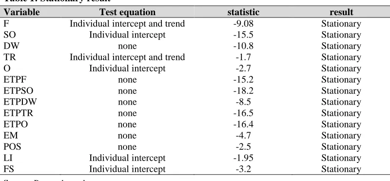
The results of stationary test using the Lin, Levin and Chu have been illustrated in table (1). The test’s equation in this research is examined based on three equations of Individual intercept, Individual intercept and trend and none, which in the best condition its result is reflected.

Table 1: Stationary result

Variable Test equation statistic result

F Individual intercept and trend -9.08 Stationary

SO Individual intercept -15.5 Stationary

DW none -10.8 Stationary

TR Individual intercept and trend -1.7 Stationary

O Individual intercept -2.7 Stationary

ETPF none -15.2 Stationary

ETPSO none -18.2 Stationary

ETPDW none -8.5 Stationary

ETPTR none -16.5 Stationary

ETPO none -16.4 Stationary

EM none -4.7 Stationary

POS none -2.5 Stationary

LI Individual intercept -1.95 Stationary

FS Individual intercept -3.2 Stationary

Source: Research results

344 Estimating the extended linear expenditures system

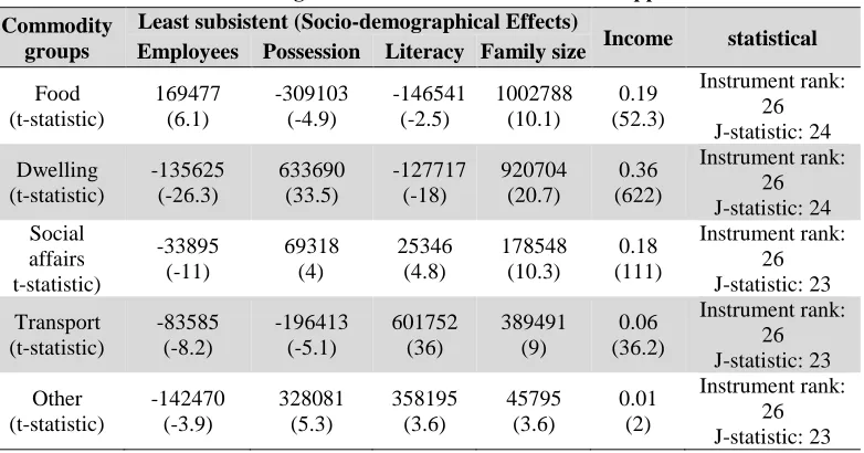
a)Estimating the subsistence level of living: Table (2) shows that the results of Engel’s equations based on equation (9) and based on the 2-stage Generalized Method of Moments (2S-GMM) indicate the complete significance of the variables.

Table: 2 Statistical results of Engel’s functions based on the GMM approach Commodity

groups

Least subsistent (Socio-demographical Effects)

Income statistical Employees Possession Literacy Family size

Food (t-statistic) 169477 (6.1) -309103 (-4.9) -146541 (-2.5) 1002788 (10.1) 0.19 (52.3) Instrument rank: 26 J-statistic: 24 Dwelling (t-statistic) -135625 (-26.3) 633690 (33.5) -127717 (-18) 920704 (20.7) 0.36 (622) Instrument rank: 26 J-statistic: 24 Social affairs t-statistic) -33895 (-11) 69318 (4) 25346 (4.8) 178548 (10.3) 0.18 (111) Instrument rank: 26 J-statistic: 23 Transport (t-statistic) -83585 (-8.2) -196413 (-5.1) 601752 (36) 389491 (9) 0.06 (36.2) Instrument rank: 26 J-statistic: 23 Other (t-statistic) -142470 (-3.9) 328081 (5.3) 358195 (3.6) 45795 (3.6) 0.01 (2) Instrument rank: 26 J-statistic: 23

Source: Research results

Details in table (2) which indicate the amount of effects of four socio-demographical variables on subsistence level of living give us important results. To simplify understanding the results, the type of obtained equation has been shown in table (3):

Table: 3 Socio-demographical variables’ effect on subsistence level of living

Food Dwelling Social affairs Transport Other

Employees Positive negative negative negative negative

Possession negative Positive Positive negative Positive

Literacy negative negative Positive Positive Positive

Family size Positive Positive Positive Positive Positive

Source: table 2

345

b) Estimating the poverty line: since in this research the panel data approach has been used for calculating the subsistence level of living, the results are examined based on separate years and declines. Thus, to calculate the annual subsistence level of living and poverty line, the average of ten income groups has been used. The subsistence level of living is calculated based on equation (5) and the poverty line is calculated based on equation (8). The results are shown in table 4.

Table: 4 Subsistence level of living changes and urban areas poverty line in Iran ($)

Year Least subsistence Monthly poverty line ($)

food dwelling social affairs transport other

1982 5.86 4.02 0.63 1.33 1.91 171.7

1983 6.19 4.03 0.59 1.02 1.67 152.2

1984 5.76 4.25 0.63 0.92 1.78 130.7

1985 5.69 4.05 0.64 1.33 1.92 131.9

1986 5.09 4.26 0.70 1.51 2.28 136.9

1987 5.10 4.23 0.66 1.18 2.03 128.8

1988 4.68 4.64 0.75 1.35 2.41 178.4

1989 5.20 5.14 0.84 1.60 2.77 188.1

1990 6.58 5.10 0.76 1.50 2.60 190.2

1991 6.19 5.02 0.78 1.61 2.63 220.2

1992 5.63 4.55 0.77 1.92 2.60 240.9

1993 6.13 4.01 0.67 2.07 2.38 243.2

1994 5.16 4.58 0.80 2.09 2.78 230.7

1995 6.08 4.77 0.81 2.34 2.97 244.9

1996 5.17 4.66 0.85 2.61 3.19 267.0

1997 6.38 3.94 0.77 3.68 3.50 318.5

1998 5.42 4.59 0.88 3.46 3.77 270.5

1999 5.57 4.94 0.91 3.38 3.93 253.4

2000 5.69 3.66 0.78 3.95 3.57 284.9

2001 5.03 4.00 0.84 3.77 3.66 321.0

2002 4.73 3.95 0.82 3.49 3.48 343.3

2003 4.54 3.85 0.77 2.97 3.10 353.6

2004 4.73 3.71 0.81 3.84 3.64 419.5

2005 4.27 3.34 0.78 4.13 3.70 436.9

2006 4.01 3.33 0.77 3.83 3.52 458.5

2007 3.65 3.15 0.71 3.27 3.08 477.8

Source: Research results

346

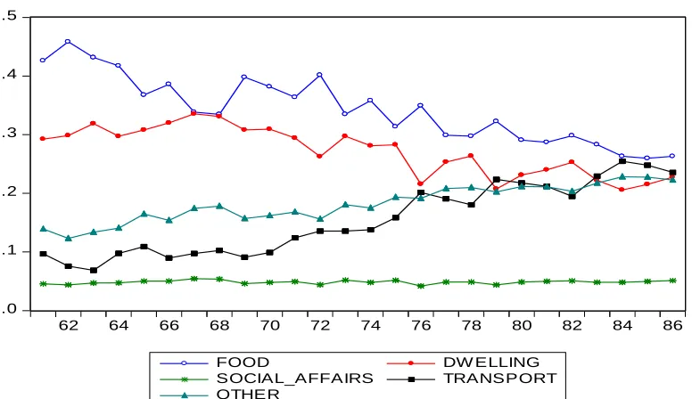
subsistence level of living has changes parallel with changes in socio-demographical variables and share of each subsistence level of living in each year is specifically different. The share of commodity subsistence level of living from the whole least subsistence indicates the degree of provision priority of that commodity group to other commodities. In the following diagram, the process of least subsistence share changes of commodity groups from the whole least subsistence has been determined.

.0 .1 .2 .3 .4 .5

62 64 66 68 70 72 74 76 78 80 82 84 86

FOOD DW ELLING

SOCIAL_AFFAIRS TRANSPORT

OTHER

Figure 1: Changes in subsistence level of living share from the total subsistence level of living

Referring to diagram 1, it is clear that during the study period the share of food and dwelling has given up their places to the transportation and other services share, i.e. the priority of meeting the basic needs such as food and dwelling, has given their place to other needs, while the share of social affairs group is remained almost fixed.

Conclusions

347

family head, and the family size on the subsistence level of living were examined. The poverty line has been estimated based on Engel’s equations through the family expenditures data on eight commodity groups which in this research have been integrated into five groups of food, dwelling, social affairs, transportation, and others. The results of Engel’s equations indicate the complete significance of variables. Two points are important about the socio-demographical variables effects on the subsistence level of living. First, the family size has a positive relationship with all of the commodity groups’ subsistence level of living, and second, while the rate of family employees has a positive relationship with commodity groups, this relationship is negative only for the food group. The most important feature about the estimation results is the increasing trend of poverty line and changes in the subsistence level of living. According to these results, the monthly poverty line for Iran urban areas has increased from 171$ in 1982 to 477$ in 2007, That is, the poverty line has increased 2.8 times during the study period. Furthermore, the results show that the trend share of commodity subsistence level of living from the whole subsistence level of living indicates the degree of priority of commodity group provision compared with other commodities. The results also show that during the food and dwelling share have given their place to the transportation and other services share during the study period, i.e. the priority of meeting basic needs, food and dwelling, is given to other needs, while the social affairs’ share has been remained fixed.

Reference

Sanoy, A., & Safa, M. S. (2005). The effectiveness of agriculture credit on the standard of living browsers in Yemen. An extended expenditure system approach. The Agriculturist, 3(1 & 2): 117-127.

Albacea, Z. (1995). Estimation of provincial poverty incidence in the Philippines. Philippine institute for development studies university of the Philippines los baños, institute of statistics college, los baños, Laguna, Philippines 403.

Arellano, M., & Bond, S. R. (1991). Some tests of specification for panel data Monte Carlo evidence and an application to employment equations. Review of Economic Studies, 58, 277-297.

Grootaert, C. (1997). The determinants of poverty in Côte d’Ivoire in the 1980s. Journal of

African Economies, (6)2, 169–196.

How, H. (1977). Cross-section application of linear expenditure systems: responses to socio demographic effects. American Journal of Agricultural Economics, 1(59), 141-148. Klein, L. R., & Rubin, H. (1947). A constant-utility index of cost of living. The Review of

348

Levin, A., & Lin, C. F. (1992). Unit root test in panel data asymptotic and finite sample properties, university of California, San Diego, DSiscussion Paper, No. 92-93.

Luch, C. (1973). The extended linear expenditure system. European Economic Review, (4), 21- 73.

MacDonald, R. (1996). Panel unit root tests and real exchange rates. Economics Letters, 50, 7-11. Madzingira, N. (1997). Poverty and aging in Zimbabwe. Journal of Social Development in

Africa, 12(2), 5–19.

Narayana, N. S. S., & Vani, B. P. (2000). Earnings and consumption by Indian rural laborers,

analysis with an extended linear expenditure system. Economic analysis unit, Indian Statistical Institute, Bangalore, India, society for policy modeling.

Oh, K. Y. (1996). Purchasing power parity and unit root tests using panel data. Journal of

International Money and Finance, 15, 405-418.

Pollak, R. A., & Wales, T. J. (1969). Estimation of linear expenditure system. Econometrica, 37(4), 611-628.

Statistical Center of Iran, Statistical Yearbook, 1983-2007.

Stone, P. (1954). Linear expenditure system and demand analysis: an application to the pattern of British demand. Economic journal, 64, 511-552.