Surrounding Word Sense Model for Japanese All-words Word Sense
Disambiguation
Kanako KOMIYA1 Yuto SASAKI2 Hajime MORITA3 Minoru SASAKI1 Hiroyuki SHINNOU1Yoshiyuki KOTANI2
1Ibaraki University2Kyoto University3Tokyo University of Agriculture and Technology
kanako.komiya.nlp@vc.ibaraki.ac.jp, 50010268030@st.tuat.ac.jp morita@nlp.ist.i.kyoto-u.ac.jp, minoru.sasaki.01@vc.ibaraki.ac.jp
hiroyuki.shinnou.0828@vc.ibaraki.ac.jp, kotani@cc.tuat.ac.jp
Abstract
This paper proposes a surrounding word sense model (SWSM) that uses the distri-bution of word senses that appear near am-biguous words for unsupervised all-words word sense disambiguation in Japanese. Although it was inspired by the topic model, ambiguous Japanese words tend to have similar topics since coarse semantic polysemy is less likely to occur than that in Western languages as Japanese uses Chi-nese characters, which are ideograms. We thus propose a model that uses the dis-tribution of word senses that appear near ambiguous words: SWSM. We embed-ded the concept dictionary of an Elec-tronic Dictionary Research (EDR) elec-tronic dictionary in the system and used the Japanese Corpus of EDR for the exper-iments, which demonstrated that SWSM outperformed a system with a random baseline and a system that used a topic model called Dirichlet Allocation with WORDNET (LDAWN), especially when there were high levels of entropy for the word sense distribution of ambiguous words.
1 Introduction
This paper proposes a surrounding word sense model (SWSM) for unsupervised Japanese all-words Word Sense Disambiguation (WSD). SWSM assumes that the sense distribution of sur-rounding words varies according to the sense of a polysemous word.
For instance, a word “ ” (possibility) has three senses according to the Electronic Dictionary Research (EDR) electronic dictionary (Miyoshi et al., 1996):
(1) The ability to do something well
(2) Its feasibility
(3) The certainty of something happenings
Although sense (3) is the most frequent in the prior distributions, sense (1) will be more likely when the local context includes some concepts
like “ ” (man) or “ ” (someone’s). It
is challenging in practice to accurately learn the difference in the senses of surrounding words in an unsupervised manner, but we developed an ap-proximate model that took conditions into consid-eration.
SWSM is a method for all-words WSD in-spired by the topic model (Section 2). It treats the similarities of word senses using WORDNET-WALK and it generates word senses of ambigu-ous words and their surrounding words (Section 3). First, SWSM abstracted the concepts of the concept dictionary (Section 4) and calculated the transition probabilities for priors (Section 5). Then it estimated the word senses using Gibbs Sam-pling (Section 6) . Our experiments with an EDR Japanese corpus and a Concept Dictionary (Sec-tion 7) indicated that SWSM was effective for Japanese all-words WSD (Section 8) . We dis-cuss the results (Section 9) and concludes this pa-per (Section 10) .
2 Related Work
There are many methods of all-words WSD. Ped-ersen et al. (2005) proposed calculation of the se-mantic relatedness of the word senses of ambigu-ous words and their surrounding words. Some papers have reported that methods using topic models (Blei et al., 2003) are most effective. Boyd-Graber et al. (2007) proposed a model, called Latent Dirichlet Allocation with WORD-NET (LDAWN), which was a model where the probability distributions of words that the topics had were replaced with a word generation pro-cess on WordNet: WORDNET-WALK. They
ap-35
29th Pacific Asia Conference on Language, Information and Computation pages 35 - 43 Shanghai, China, October 30 - November 1, 2015
plied the topic model to unsupervised English all-words WSD. Although Guo and Diab (2011) also used the topic model and WordNet, they also used WordNet as a lexical resource for sense definitions and they did not use its conceptual structure. They reported that the performance of their system was comparable with that reported by Boyd-Graber et al.
There has been little work, on the other hand, on unsupervised Japanese all-words WSD. As far as we know, there has only been one paper (Bald-win et al., 2008) and there have been no reported methods that have used the topic model. We think this is because ambiguous words in Japanese tend to have similar topics since coarse semantic poly-semy is less likely to occur compared to that with Western languages as Japanese uses Chinese char-acters, which are ideograms. In addition, Guo and Diab (2011) reported that in word sense disam-biguation (WSD), an even narrower context was taken into consideration, as Mihalcea (2005) had reported. Therefore, we assumed that the word senses of the local context are differentiated de-pending on the word sense of the target word like that in supervised WSD. SWSM was inspired by LDAWN, it thus uses WORDNET-WALK and Gibbs sampling but it does not use the topics but the word senses of the surrounding words. We pro-pose SWSM as an approach to unsupervised WSD and carried out Japanese all-words WSD.
3 Surrounding Word Sense Model
SWSM uses the distribution of word senses that appear near the target word in WSD to estimate the word senses assuming that the word senses of the local context are differentiated depending on the word sense of the target word. In other words, SWSM estimates the word sense accord-ing top(s|w), which is a conditional probability of a string of senses,s, given a string of wordsw. SWSM involves three assumptions. First, each word sense has a probability distribution of the senses of the surrounding words. Second, whenci
denotes the sense string of the surrounding words of the target wordwi, the conditional probability
of ci given wi is the product of the those of the
senses in ci givenwi. For example, when wi is
“ ” (possibility) and its surrounding words
are “ ” (both sides) and “ ” (human),
ci = (sboth, shuman) and P(ci|spossibility) = P(sboth|spossibility)P(shuman|spossibility) are
de-fined wherespossibility,sboth, and shuman denote
word senses of “ ” (possibility), “ ”
(both sides), and “ ” (human). Finally, each polyseme has a prior distribution of the senses. Given these assumptions, SWSM calculates the conditional probability ofsthat corresponds tow, under the condition wherewis observed as:
P(s,c|w) = N ∏
i=1
P(si|wi)P(ci|si,w), (1)
wherecdenotes the string ofciandN denotes the
number of all the words in the text. The initial part on the right is the probability distribution of the word sense of each word and the last part is that of the senses of the surrounding words for each word sense. We set the Dirichlet distribution as their prior.
The final equation considering prior is de-scribed using the following parameters:
P(s,c,θ,φ|w, γk, τj) =
W ∏
k=1
P(θk|γk) S ∏
j=1
P(φj|τj) N ∏
i=1
P(si|θwi)P(ci|φsj,w),
(2) where W denotes the number of words, S de-notes the number of senses, θk denotes the
prob-ability distribution of the senses of word k, and
φjdenotes the probability distribution of the word
senses surrounding word sensej.θkandφjare the
parameters of the multinomial distribution. γ and
τ are the parameters of the Dirichlet distribution.
Eq. (2) is the basic form. We
re-place φ, the probability distribution of each sense, with the generation process by using the WORDNET-WALK of the concept dictionary. The WORDNET-WALK in this work does not generate words but word senses using a hyper-transition probability parameter, Sα. We set α
according to the senses to differentiate the sense distribution of the surrounding words before train-ing. By doing this, we can determine which sense in the model corresponds to the senses in the dic-tionary.
SWSM estimates the word senses using Gibbs sampling as:
(1) Pre-processing
Figure 1: Example of WORNET-WALK
2 Calculate the transition parameters using the sense frequencies
(2) Training: Gibbs sampling to estimate the word senses
4 Concept Abstraction
SWSM obtains the sense probability of the surrounding words using WORDNET-WALK. WORDNET-WALK involves the generation pro-cess, which represents the probabilistic walks over the hierarchy of conceptual structures like Word-Net. Figure 1 shows the easy example of the generation probabilities of words by WORDNET-WALK. When circle nodes represent concepts and triangle nodes represent words of leaf concepts ,i.e., X and Y, and numbers represent the transi-tion probabilities, the generatransi-tion probabilities of words A, B, C, and D are 0.03 0.27 0.28 and 0.42. LDAWN calculated the probabilities of word senses using the transition probability from the root node in a concept dictionary. WORDNET-WALK generated words in (Boyd-Graber et al., 2007) but our WORDNET-WALK generates word senses. However, the word senses sometimes do not correspond to leaf nodes but to internal nodes in our model and that causes a problem: the sum of the probabilities is not one. Thus, we added leaf nodes of the word senses directly below the inter-nal nodes of the concept dictionary (c.f. Figure 2). Concept abstraction involves the process by which hyponym concepts map onto hypernym concepts. Most concepts in a very deep hierar-chy are fine grained like the “Tokyo University of Agriculture and Technology” and “Ibaraki Univer-sity” and they should be combined together like “university” to avoid the zero frequency problem.
Figure 2: Addition of Word Sense Nodes
Thus, SWSM combines semantically similar con-cepts in the concept dictionary.
Hirakawa and Kimura (2003) reported that they compared three methods for concept abstraction, i.e, flat depth, flat size, and flat probability meth-ods, by using the EDR concept dictionary, and the flat probability method was the best. Therefore, we used the flat probability method for concept ab-straction.
The flat probability method consists of two steps. First, there is a search for nodes from the root node in depth first order. Second, if the con-cept probability calculated based on the corpus is less than a threshold value, the concept and its hyponym concepts are mapped onto its hypernym concept.
We employed the methods of (Ribas, 1995) and (McCarthy, 1997) to calculate the concept prob-ability. Ribas (1995) calculated the frequency of sensesas:
f req(s) =∑ w
|senses(w)∈U(s)|
|senses(w)| count(w),
(3) wheresenses(w)denotes the possible senses of a wordw,U(s)denotes conceptsand its hyponym concepts, andcount(w)denotes the frequency of word w. This equation weightscount(w) by the ratio of conceptsand its hyponym concepts in all the word senses ofw. probabilityP(si) was cal-culated as:
P(si) = f req(si)
N , (4)
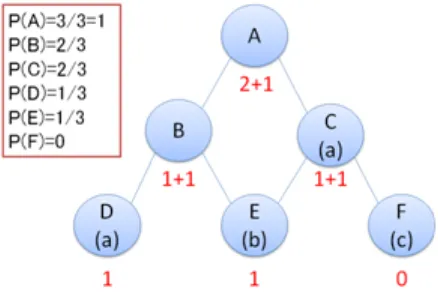
whereN denotes the number of word tokens. Figure 3 demonstrates the example of the con-ceptual structure1. The nodes A∼F represent the
Figure 3: Example of Concept Structure
concepts and (a)∼(c) represent the words, which indicates that word (a) is a polyseme that have two word senses, i.e., C and D. When word (a) appeared twice and word (b) appeared once, the probabilities are as illustrated in Figure 3. Note that C and D share the frequencies of word (a).
A Turing estimator (Gale and Sampson, 1995) was used for smoothing with rounding of the weighted frequencies.
Concept abstraction sometimes causes a prob-lem where some word senses of a polyseme are mapped onto the same concept. The most frequent sense in the corpus has been chosen for the answer in these cases.
5 Transition Probability
SWSM differentiates the sense distribution of the surrounding words of each target word before training usingα: the transition probability param-eter. As our method is an unsupervised approach, we cannot know the word senses in the corpus. Therefore, SWSM counts the frequencies of all the possible word senses of the surrounding words in the corpus. That is, if there are polysemes A and B in the corpus and B is a surrounding word of A, SWSM counts the frequencies of the senses by considering that all the senses of B appeared near all the senses of A. That makes no difference in the sense distributions of A; however, if there is another polyseme or a monosemic word, C, and a sense of C is identical with a sense of A, the sense distributions of A will be differentiated by count-ing the frequencies of the senses of C. As this ex-ample indicates, SWSM expects that words that have an identical sense, like A and C, have similar local contexts.
SWSM uses these counted frequencies to cal-culate the transition parameterαso that the transi-tion probabilities to each concept are proportransi-tional to the word sense frequencies of the surround-ing words. We calculateαsi,sj, i.e., the transition
probability from hypernymsito hyponymsj, like
that in (Jiang and Conrath, 1997) as:
αsi,sj =P(sj|si) =
P(si, sj) P(si)
= P(sj) P(si)
. (5)
In addition, probabilityP(si)is calculated as:
P(si) =
f req(si)
N , (6)
wheref req(si)denotes the frequency of sensesi.
Moreover, f req(si) is calculated like that in
(Resnik, 1995):
f req(si) = ∑ w∈words(si)
count(w). (7)
Here, words(si) denotes a concept set that
in-cludes si and its hyponyms, and N denotes the
number of the word tokens in the corpus. How-ever, the probability that Eq. (7) will have a prob-lem, i.e., the sum of the transition probabilities from a concept to its hyponyms is not one. Thus, we calculate the probability by considering that the same concept that follow a different path is dif-ferent:
f req(si)= ∑
sj∈L(si)
path(si,sj) ∑
w∈words(si)
count(w),
(8) where path(si, sj) denotes the number of the
paths from conceptsito its hyponymsjandL(si)
denotes the leaf concepts belowsi. Consequently,
the transition probability can be calculated by di-viding the frequencies of the hyponym by that of its hypernym.
When word (a) appeared twice and word (b) ap-peared once, the transition probability from A to B, i.e.,αA,B is 1/2 because the frequencies of A
and B are six2and three in Figure 3.
Here,p(pathsl), i.e., a transition probability of
an arbitrary path from the root node to a leaf con-cept,pathsl, is:
p(pathsl)
of target words according to difficulty. Only words that appeared more than four times in the corpus were classified based on difficulty.
Difficulty Entoropy
Easy E(w)<0.5
Normal 0.5≤E(w)<1
Hard 1≤E(w)
Table 2: Difficulty of disambiguation
Difficulty Word types Tokens(N) Tokens(V) All 4,822 12,149 6,199 Easy 399 3,630 1,723 Normal 337 2,929 1,541 Hard 105 1,028 1,196
Table 3: Types and tokens of words according to difficulty
Difficulty Noun polysemy Verb polysemy
All 4.2 5.5
Easy 3.9 4.0
Normal 4.4 5.3
Hard 8.6 10.3
Table 4: Average polysemy of target words ac-cording to difficulty
8 Result
We used nouns and independent verbs in a local window whose size was2N except for marks, as the surrounding words. We set N = 10 in this research. In addition, we deleted word senses that appeared only once through pre-processing.
We performed experiments using the nine set-tings of the transition probability parameters:
Sa={1.0,5.0,10.0}andSb ={10.0,15.0,20.0}
in Eq.(10). We set the hyper-parameterγ= 0.1in Eq.(2) for all experiments. Gibbs sampling was it-erated 2,000 times and the most frequent senses of 100 samples in the latter 1,800 times were chosen for the answers. We performed experiments three times per setting for the transition probability pa-rameters and calculated the average accuracies.
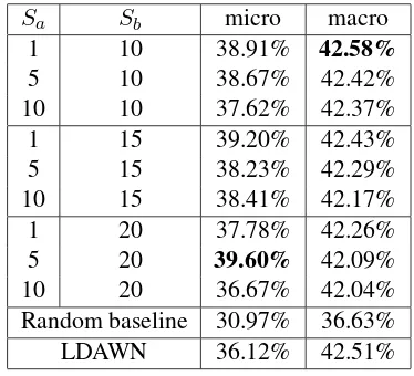
Table 4 summaries the results. It includes the micro- and macro-averaged accuracies of SWSM for the nine settings of the parameters, those of the
random baseline, and those of LDAWN5. The ex-periments for the random baseline were performed 1,000 times. The best results are indicated in bold-face.
Sa Sb micro macro
1 10 38.91% 42.58%
5 10 38.67% 42.42%
10 10 37.62% 42.37%
1 15 39.20% 42.43%
5 15 38.23% 42.29%
10 15 38.41% 42.17%
1 20 37.78% 42.26%
5 20 39.60% 42.09%
10 20 36.67% 42.04%
Random baseline 30.97% 36.63%
LDAWN 36.12% 42.51%
Table 5: Summary of result
The table indicates that our model, SWSM, was better than both the random baseline and LDAWN. Although the macro-averaged accura-cies of LDAWN were better than those of SWSM except when Sa = 1 and Sb = 10, both the
micro- and macro-averaged accuracies of SWSM outperformed those of LDAWN whenSa= 1and Sb = 10.
Tables 5 and 6 summarize the micro-averaged accuracies of all words and the macro-averaged accuracies of all words. SWSM1 and SWSM2 in these tables denote the SWSMs with the set-ting when the best macro-averaged accuracy for all words was obtained (Sa= 1andSb = 10) and
with the setting when the best micro-averaged ac-curacy for all words was obtained (Sa = 5 and Sb = 20). The best results in each table are
indicated in boldface. These tables indicate that SWSM1 or SWSM2 was always better than both
5
the random baseline and LDAWN.
Method All Easy Normal Hard
Random 30.97 33.01 29.35 13.47
LDAWN 36.12 42.06 30.66 13.52
SWSM1 38.91 46.87 33.44 19.92
SWSM2 39.60 48.90 32.85 23.95
Table 6: Micro-averaged accuracies for all words (%)
Method All Easy Normal Hard
Random 36.63 36.91 32.09 16.03
LDAWN 42.51 44.65 34.83 17.80
SWSM1 42.58 44.78 36.38 21.06
SWSM2 42.09 43.68 36.01 20.44
Table 7: Macro-averaged accuracies for all words (%)
Table 6 indicates that the macro averaged accu-racies of LDAWN (42.51%) outperformed those of SWSM2 (42.09%) when all the words were evaluated. However, the same table reveals that the reason is due to the results for the easy class words, i.e., the words that almost always had the same sense. In addition, Tables 5 and 6 indicate that SWSM clearly outperformed the other sys-tems for words in the normal and hard classes.
9 Discussion
The examples“ (possibility)” and “
(wash)” were cases where most senses were cor-rectly predicted. “ (possibility)” is a hard-class word and it appeared 18 times in the corpus. SWSM correctly predicted the senses of∼70% of them. It had three senses as described in Section 1: (1) the ability to do something well, (2) its fea-sibility, and (3) the certainty of something hap-penings. First, SWSM could correctly predict the first sense. The words that surrounded them were, for instance, “ (both sides)” and “
(hu-man)”, and “ (research)”, “
(in-dustrial complex)”, and “ (hereafter)”. Sec-ond, SWSM could correctly predict almost none of the words that had the second sense. The words surrounding an example were “ (every day)”,
“ (various)”, “ (to face)”, and “
(people)”, and SWSM predicted the sense as sense (1). We think that “ (people)” misled the an-swer. The words surrounding another example
were “ (break through)”, “ (music)”, and “ (spread)”, and SWSM predict the sense as sense (1). We think that “ (spread)” could be a clue to predict the sense, but “ (music)” misled the answer because it appeared many times in the corpus. Finally, SWSM could correctly pre-dicted the last sense. The words surrounded them were, for instance, (1) “ (situation)”, “ (arise)”, and “ (appear)”, (2) “ (apprecia-tion)”, “ (escalate)”, and “ (appear)”, and
(3) “ (read)” and“ (deny)”.
“ (wash)” is a normal-class word and it ap-peared five times in the corpus. SWSM correctly predicted the senses of∼80%, viz., four of them. It has two senses in the corpus: (1) sanctify (some-one’s heart) and (2) wash out a stain with wa-ter. The words surrounding the example that were incorrectly predicted were “ (tonight)”, “ (body)”, and “ (not)”, and SWSM answered the sense as (1) even though it was (2). The words surrounding the examples that were correctly pre-dicted were (1) “ (islander)”, “ (tear)”, and “ (stone)”, (2) “ (look at)” and “ (heart)”, (3) “ (limb)”, “ (face)”, “ (I)”, and “ (bath)”, (4) “ (body)”, “ (water)”, and “ (drain)”.
These examples demonstrate that the surround-ing words were good clues to disambiguate the word senses.
10 Conclusion
References
Timothy Baldwin, Su Nam Kim, Francis Bond, Sanae Fujita, David Martinez, and Takaaki Tanaka. 2008. Mrd-based word sense disambiguation: Further ex-tending lesk. In Proceedings of the 2008 Interna-tional Joint Conference on Natural Language Pro-cessing, pages 775–780.
David Blei, Andrew Ng, and Michael Jordan. 2003. Latent dirichlet allocation. Journal of Machine Learning Research, 1(3):993–1022.
Jordan Boyd-Graber, David M. Blei, and Xiaojin Zhu. 2007. A topic model for word sense disambiguation. In Proceedings of the 2007 Joint Conference on Empirical Methods in Natural Language Process-ing and Computational Natural Language LearnProcess-ing, pages 1024–1033.
W. Gale and G. Sampson. 1995. Good-turing smooth-ing without tears. Journal of Quantitative Linguis-tics, 2(3):217–237.
Weiwei Guo and Mona Diab. 2011. Semantic topic models: Combining word distributional statistics and dictionary definitions. In Proceedings of the 2011 Conference on Empirical Methods in Natural Language Processing, pages 552–561.
Hideki Hirakawa and Kazuhiro Kimura. 2003. Con-cept abstraction methods using conCon-cept classifica-tion and their evaluaclassifica-tion on word sense disam-biguation task. IPSJ Journal, 2(44):421–432, (In Japanese).
Jay J. Jiang and David W. Conrath. 1997. Semantic similarity based on corpus statistics and lexical tax-onomy. InProceedings of International Conference Research on Computational Linguistics, pages 19– 33.
Jun S Liu. 1994. The collapsed gibbs sampler in bayesian computations with applications to a gene regulation problem. Journal of the American Statis-tical Association, 427(40):958–966.
Diana McCarthy. 1997. Estimation of a probability distribution over a hierarchical classification. InThe Tenth White House Papers COGS - CSRP, pages 1– 9.
Rada Mihalcea. 2005. Unsupervised large-vocabulary word sense disambiguation with graph-based algo-rithms for sequence data labeling. InProceedings of the 2005 Conference on Empirical Methods in Nat-ural Language Processing, pages 411–418.
Hideo Miyoshi, Kenji Sugiyama, Masahiro Kobayashi, and Takano Ogino. 1996. An overview of the edr electronic dictionary and the current status of its uti-lization. InProceedings of the COLING 1996 Vol-ume 2: The 16th International Conference on Com-putational Linguistics, pages 1090–1093.
Ted Pedersen, Satanjeev Banerjee, and Siddharth Pat-wardhan. 2005. Maximizing semantic relatedness to perform word sense disambiguation. InResearch Report UMSI.
Philip Resnik. 1995. Using information content to evaluate semantic similarity in a taxonomy. In Inter-national Joint Conferences on Artificial Intelligence, pages 448–453.
Francesc Ribas. 1995. On learning more appropriate selectional restrictions. In Proceedings of the Sev-enth Conference of the European Chapter of the As-sociation for Computational Linguistics, pages 112– 118.
Yuto Sasaki, Kanako Komiya, and Yoshiyuki Kotani. 2014. Word sense disambiguation using topic model and thesaurus. In Proceedings of the fifth corpus Japanese workshop, pages 71–80 (In Japanese).