Technical Article
Quantitation of 3D ureteric branching morphogenesis
in cultured embryonic mouse kidney
LUISE A. CULLEN-M
CEWEN
1,
GABRIEL FRICOUT
2, IAN S. HARPER
1, DOMINIQUE JEULIN
2and JOHN F. BERTRAM*
,11Department of Anatomy and Cell Biology, Monash University, Clayton, Victoria, Australia and 2Centre de Morphologie Mathématique, Ecole des Mines de Paris, France
ABSTRACT The growth and branching of the epithelial ureteric tree is critical for development of the permanent kidney (metanephros). Current methods of analysis of ureteric branching are mostly qualitative. We have developed a method for measuring the length of individual branches, and thereby the total length of the ureteric tree in 3 dimensions (3D). The method involves confocal microscopy of whole-mount immunostained metanephroi and computer-based image segmenta-tion, skeletonisation and measurement. The algorithm performs semi-automatic segmentation of a set of confocal images and skeletonisation of the resulting binary object. Length measurements and number of branch points are automatically obtained. The final representation can be recon-structed providing a fully rotating 3D perspective of the skeletonised tree. After 36 h culture of E12 mouse metanephroi, the total length of the ureteric tree was 6103 ±±±±± 291 µµµµµm (mean±±±±±SD), a four-fold increase compared with metanephroi cultured for just 6 h (1522 ±±±±± 149 µµµµµm). Ureteric duct length increased at a rate of 153 µµµµµm/h over the first 30 h period and was maximal between 18 and 24 h at 325 µµµµµm/h. The distribution of branch lengths at the six time points studied was similar, suggesting tight control of ureteric lengthening and branching. This method will be of use in analysing ureteric growth in kidneys cultured in the presence of specific molecules suspected of regulating ureteric growth. The method can also be used to analyse in vivo kidneys and to quantify branching morphogenesis in other developing organs.
KEY WORDS:
branching, image analysis, kidney development
0214-6282/2002/$25.00
© UBC Press Printed in Spain
www.ijdb.ehu.es
*Address correspondence to: John F. Bertram, PhD. Department of Anatomy and Cell Biology, School of Biomedical Sciences, Monash University, Clayton, Victoria, Australia 3800. Fax: +61-3-9905-2766. e-mail: [email protected]
Abbreviations used in this paper: 3D, three dimensional; TVP, total vertical
projection.
Introduction
Branching morphogenesis is a key event in the development of many epithelial organs, including the lung, prostate gland, mam-mary gland, salivary gland and kidney. The branching pattern within each organ is generally considered to be highly organised, and certainly is important in establishing the characteristic histoarchitecture of the adult organ.
The development of the permanent kidney (metanephros) is characterised by a series of inductive interactions between the epithelial ureteric bud and the metanephric mesenchyme. The epithelial bud emerges from the Wolffian duct and grows caudally into the adjacent mesenchyme. The mesenchymal cells induce growth and branching of the ureteric bud. Through repeated branching, the ureteric bud ultimately gives rise to the collecting duct system of the kidney and the ureter. Simultaneously, the tips of the branching duct induce the surrounding mesenchyme to condense, epithelialise and differentiate into nephrons. Current understanding of the genetic and molecular regulation of kidney
development has been described in a number of recent reviews
(Davies and Davey, 1999; Horster et al., 1999; Burrow, 2000; Clark
and Bertram, 2000; Kuure et al., 2000).
Ureteric branching morphogenesis in the developing metaneph-ros is believed to be a major determinant of the total number of nephrons that form in the metanephros. After successive genera-tions of branching, the normal human kidney can contain between 300,000 and over 1 million nephrons (Nyengaard and Bendsten, 1992). Reduced nephron number has been associated with the
development of essential hypertension (Brenner et al., 1988), chronic
renal failure (Brenner et al., 1988, Brenner and Chertow, 1994) and
The molecular regulation of metanephric development and ure-teric branching morphogenesis has been extensively studied using whole metanephric organ culture. However, despite the utility of metanephric organ culture as a model for defining the roles of specific molecules in ureteric branching morphogenesis, the growth and structure of the ureteric tree is most often described in subjective and qualitative terms. Moreover, those quantitative methods that are available do not take into account the 3-dimensional (3D) shape of the ureteric “tree”.
We have developed a new method for analyzing ureteric tree lengths in 3D. A preliminary report describing the algorithm perform-ing semi-automatic skeletonisation and preliminary ureteric tree length measurements for 10 kidneys cultured for 12 and 24 hours has
previously been published (Fricout et al., 2001). The present report
describes an improved version of the method for measuring in 3D the growth of the mouse ureteric tree, and a full set of data demonstrating ureteric tree length measurements over six time periods. We have used the method to measure branches in embryonic day 12 (E12) mouse metanephroi cultured for up to 48 h. The data suggest tight regulatory control of branch initiation and lengthening which ulti-mately results in the recognizable architectural ‘pattern’ of the ureteric tree.
Experimental Protocols
Animals
Whole mouse (Balbc) kidneys were obtained at E12. Embryonic bodyweights were restricted to 0.060-0.080 g prior to culture.
washing, metanephroi were mounted whole on a cavity slide.
Confocal Microscopy
Whole metanephroi were optically sectioned parallel to the polycarbon-ate filter with a 10x lens on a Leica TCS NT confocal microscope. Since the lens has a measured axial resolution
(FWHM) of 10 µm, sections were taken
at intervals of 5 µm to satisfy the
re-quirements for Nyquest sampling. The resulting 2D optical slices were 8 bit (256 grey level) images, typically 512 x 512 pixels (Fig. 1A). Between 20 and 60 images were required to sample each metanephros.
Image Analysis
Binarisation Production of the binary images used to produce skeletons was done using MicroMorph for Windows (Version 1.4) developed by the Centre de Morphologie Mathématique, Ecole des Mines de Paris, France.
The main image analysis steps were as follows:
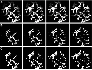
Production of ‘Maximum’ Images: To remove additional information com-ing from the depth of each section, the confocal (grey level) images were
Fig. 1. Binarisation of confocal images.Four consecutive grey level images (A) are first converted to
‘maximum’ images by selecting those X,Y points which are at their maximal intensity and therefore at the correct depth (B). These maximum images are then converted to binary images (C) through thresholding and smoothing using a filtering parameter.
Bodyweight restrictions have proven reliable in our laboratory in reducing variation in metanephric size and therefore metanephric development, thereby increasing the statistical power of experi-ments. Metanephroi were cultured on polycarbonate filters (Transwell, Corning Star Corporation, Cambridge, Massachusetts, USA) for up to 48 h (6, 12, 18, 24, 36 and 48 h) in serum-free Dulbecco’s modified Eagle’s medium (DMEM): Ham’s F12 liquid medium (Trace
Bio-sciences, Castle Hill, NSW, Australia) supplemented with 5 µg/ml
transferrin (Sigma-Aldrich Pty. Ltd., Castle Hill, Australia) and 12.9 µl/
ml L-glutamine (Trace Biosciences, Castle Hill, NSW, Australia), 100
µg/ml penicillin/ 100 U/ml streptomycin (Trace Biosciences) and 5
mg/ml transferrin (Sigma-Aldrich Pty. Ltd., Castle Hill, Australia), at
37°C and 5% CO2. Culture media was changed every 24 h. All
experiments were approved in advance by a Monash University animal ethics committee and were conducted in accordance with the “Australian Code of Practice for the Care and Use of Animals for Scientific Purposes.”
Immunofluorescence
At the end of the culture period metanephroi were fixed in 100%
methanol at -20°C for 15 minutes. After washing in PBS for 15
minutes at room temperature non-specific binding was blocked using 5% fetal calf serum (FCS) in PBS. To visualise the branches of the ureteric tree, whole metanephroi were incubated in primary antibody
Calbindin-D28K (Sigma-Aldrich Pty. Ltd., Castle Hill, Australia) at
1:200 for 2 h at 37°C. After washing overnight at 4°C metanephroi
were incubated in secondary antibody; Alexa 488 goat anti-mouse
IgG (Molecular Probes) at a dilution of 1:100 for 2 h at 37°C. After
A
B
binarised image was first superimposed on the maximum projec-tion allowing the missing binarised areas evident on the maximum image to be corrected with considerable accuracy.
3D SkeletonisationThe second and main part of the algorithm involved construction of a 3D skeleton of the tree, which is a representation of the original tree using thin lines connected through the centre of each branch. The skeletonisation algorithm is based on image processing libraries developed in the Centre de
Morphologie Mathématique (Fricout et al., 2001) and is run on a
Linux operating system (Linux 7). The method to process a skeleton was to first find pixels centred within the tree and then to connect these pixels by a path also centred within the tree. These steps are described below:
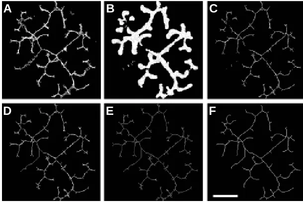
(1) Due to the differing scale of the images in the X and Y plane compared to the Z axis of the 3D object, the calculation of the centred pixels was made firstly according to the X and Y directions. Based on a distance function of an object, the algorithm first calculates the 2D skeleton of each frame by finding pixels centred in the X,Y directions within the binary image and then connecting these pixels. The resulting skeleton is centred and connected most of the time (Fig. 2A).
(2) To convert the skeleton into 3D, the pixels centred in the Z axis were then selected (Fig. 2B).
(3) The intersection of these two sets of pixels (2D skeleton and pixels centred in the Z axis) are then processed resulting in an image containing pixels centred in all three directions (X, Y and Z) (Fig. 2C). (4) These disconnected segments are linked using the path of minimum length between two pixels whose voxels are all contained within the tree. Linking all the disconnected segments of this set completes the skeleton, but the result is somewhat noisy due to small irregularities in the segmentation (Fig. 2D).
(5) The first cleaning phase thins lines which are wider than one pixel (Fig. 2E).
(6) Detecting branch points. A branch point is defined as a pixel which has three or more neighbouring pixels. When there are no longer two neighbouring pixels, these branches are labelled termi-nal branches. The bulbous endings of branches often generated two small branches in the skeleton, which is biologically inaccurate. Most of these excess branches are pruned with a final cleaning process where terminal branches are pruned if their length is less than a limit fixed by the user (Fig. 2F).
A text file produced by the algorithm provides all the branch points stored in an array with the address of the pixels of the branch arriving at one node and the length of this branch in number of pixels. Individual lengths are automatically converted to micrometres according to the placement of each individual pixel in 3D space. The final representation of the ureteric tree can be reconstructed by means of 3D volume rendering software, which allows a full rotating 3D perspective of the skeletonised tree. For this purpose we employed the use of Eikona3D (AlphaTec, Version 4) a soft-ware package for 3D image processing, analysis and visualization.
Total Vertical Projections
To check the accuracy of length measurements taken from the skeletons, we employed the stereological method of total vertical projections (TVP) (Cruz-Orive and Howard, 1991). Briefly, the TVP
method provides estimates of length density (LV; length per volume)
without knowledge of the thickness of the sections or physical slices through the specimen. Firstly, a convenient vertical axis is defined. In the case of the cultured metanephros we chose this to be parallel to the first branch or trunk. Then, with a random starting position and with uniform intervals the skeletonised ureteric tree is projected onto
a plane in a systematic set of directions between 0° and 180°, all
Fig. 2. Skeletonisation procedure.Each binary image is first skeletonised in 2D by
selecting points centred in both the X and Y directions (A). To implement into 3D, those points centred in the Z axis are then selected (B). The intersection between those points centred in X,Y and those centred in Z are then selected (C). Connection of different segments by path of minimum distance within the tree (D). The first cleaning phase thins lines to a single pixel (E). Final cleaning phase removes all terminal branches less than a limit fixed by the user (F). This is the image which is measured. Note: all images are sums of all frames for a kidney cultured for 36 h. Bar, 250 µm.
first converted to ‘maximum’ images. That is, for each (X,Y) pixel in 2D, the pixel was in focus and therefore at the correct depth (Z) when the pixel was displayed at the maximum intensity. Conversely, the pixel was out of focus when at a grey scale less than this maximum. The pixels with the same coordinates in all frames are kept if they realise the maximum intensity of this grey level function. All pixels inferior to the maximum are dis-carded and turned black. This process is conducted for each pixel in the X,Y plane, keeping only those in the Z axis which are at their maximum intensity (Fig. 1B).
Segmentation of the ‘Maximum’ Images: The next step of the algorithm involved segmenting (binarising) each frame (Fig. 1C). The tree is selected by taking the maximum of the greyscale image (described above), in addition to a threshold of these images where the threshold level is chosen according to the maximum projection of all the images. In addition to thresholding the image a filtering parameter was used to smooth the result, minimising irregularities in the segmentation.
Interactive Correction of the Result: Regions within the tree with less intense staining, such as those of the trunk, were often lost with binarisation of the maximum image. These discontinuous sections required manual correction. Interactive corrections to the segmented binary images can be made frame by frame. The
A
B
C
perpendicular to the vertical axis. These images are the TVPs. On each TVP, a cycloid test system is superimposed with uniform random position, where the shorter principal axis of the cycloids is perpendicular to the fixed vertical direction. Intersections of the skeletonised tree with the cycloid arcs in each TVP are counted. The length of the ureteric tree is then estimated using the formula:
Li = 2 x (a/l) x M-1 x n-1 x I
i where
a/l is the known ratio of test area to test line length for the test system used M is the magnification of the TVPs
n is the number of TVPs analysed, and
Ii is the number of intersections between the cycloid arcs and the ureteric tree skeleton.
Statistics
Length estimates and number of branch points were analysed using a one-way analysis of variance. Where a difference was identified, the Tukey test was used to locate the difference(s). Comparisons between TVP and values obtained with the algo-rithm were analysed using a student’s T-test. Chi-square tests were used to analyse the distribution data for both length distribu-tion and contribudistribu-tion to total length. A probability of 0.05 or less
was accepted as statistically significant. Values are mean ±
standard deviation (SD).
Results and Discussion
We have developed a new quantitative method for measuring in 3D the lengths of individual ureteric branches and the total length of the ureteric tree in the developing mouse metanephros. The tech-nique involves: (1) whole mount immunofluorescent staining of the ureteric tree; (2) optical sectioning of the whole tree using confocal microscopy; (3) conversion of the grey level images to binary images; (4) skeletonisation of each 2D optical section; (5) implementation into 3D; (6) identification of branch points resulting in a final 3D skeleton; and (7) computerised 3D measurement of the length of the whole skeleton and individual branches. The data generated with this new method represent quantitative 3D measurements of ureteric duct growth and branching.
Goodness of Fit of Skeletons
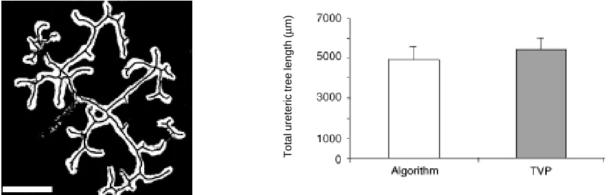
The method was able to repeatedly generate skeletons that closely matched the ureteric trees. Figure 3 shows the skeleton of
Fig. 3. (Left) Final skeleton. Superposition of the skeleton onto the original confocal image. Bar, 250 µm.
Fig. 4.(Right) Estimates of total ureteric tree length obtained with the skeletonisation algorithm and total vertical projections (TVP). Values
are for 10 E12 kidneys cultured for 24 h. The values are not significantly different.
the ureteric tree of a mouse metanephros cultured for 36 h superimposed on the original confocal image. The skeleton is observed to be thin and centred within each branch.
Precision, Accuracy and Reproducibility of Length Measurements
Importantly, the length estimates obtained were precise, accu-rate and reproducible. With regards to precision, the standard deviations of total ureteric length were on average just 11% of the mean values. Length estimates obtained with the technique were highly reproducible. Repeat measures of two E12 mouse kidneys cultured for 24 h differed by just 1 or 2% (Table 1). Estimates of total ureteric tree lengths obtained with image analysis algorithms and TVP for 10 metanephroi cultured for 24 h are shown in Fig. 4. No significant difference between the two sets of estimates was observed (p=0.28). Furthermore, estimates for branch point num-ber given by the algorithm also showed excellent agreement with manual estimates. Taken together, the precision, accuracy and reproducibility of the estimates, suggest this technique will facili-tate the detection of slight changes in ureteric tree growth in future studies.
In Vitro Growth of the Ureteric Tree
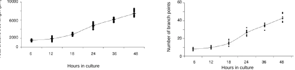
Ureteric branching and growth was analysed in 60 mouse metanephroi cultured for 6, 12, 18, 24, 36 or 48 h. It was essential that each metanephros be contained within the 512 x 512 pixel frame for laser scanning confocal microscopy. Unfortunately, many of the 48 h cultures failed to fit within this frame and were excluded from the study. Therefore, data presented for 48 h are underestimates and all mean values and growth rates will be presented without this data unless otherwise stated. Data for all six time periods are shown in Table 2 and Fig. 5. Note that measure-ments on uncultured E12 metanephroi were attempted. However, while specific staining of ureteric epithelium was achieved in uncultured E12 explants high background staining was also ob-served. This background staining made binarisation unreliable and accurate measurement problematic. Total ureteric duct length increased substantially over the culture period (p<0.001). Between
6 and 36 h, total tree length increased by approximately 4500 µm,
a 4-fold increase. There was no significant difference in total ureteric tree length between 6 and 12 h of culture. However,
Total ureteric tree length (
µ
between 12 and 18 h, 18 and 24 h and 24 and 36 h the ureteric tree significantly increased in length (p<0.05). Ureteric tree length
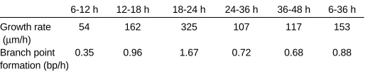
increased between 6 and 36 h at an average rate of 153 µm/hr.
Growth was maximal between 18 and 24 h at 325 µm/ h after which
the rate of growth rapidly declined (Table 3).
The extent of ureteric growth in vitro under control conditions
was somewhat surprising. After just 36 h of culture, the ureteric duct was approximately 6.1mm in length, a 4-fold increase in length in 30 h culture. Interestingly, maximal growth was observed be-tween 18 and 24 h, after which ureteric growth continued but at a slower rate. The reasons for this slowing in growth are not known,
but presumably reflect the impact of the in vitro environment
(versus the in vivo environment) including the lack of blood supply,
and perhaps the inhibition of diffusion of nutrients in the enlarging explant.
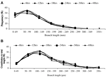
As expected, branch point number increased throughout the culture period (Fig. 6). At 6 h, ureteric trees contained an average 8 branch points, compared with 35 branch points at 36 h, a more than 4-fold increase. Branch points formed at an average rate of 0.9 branches/h. The maximum rate (1.67 branch points/h) occurred between 18 and 24 h. This coincided with the period of highest ureteric duct growth. The rate of branch point formation fell be-tween 24 and 36 h to approximately 0.7 branch points/ h (Table 3). The distribution of individual branch lengths was very similar for all culture groups (Fig. 7A). Chi-square tests showed the distribu-tions to be not significantly different. For all six groups, most
branches (∼33%) were between 50 and 99 µm in length,
irrespec-tive of their generation. 83% of branches were less than 150 µm in
length, 10% were between 150-199 µm and the remaining 7% were
200 µm or longer. Figure 7B shows the contributions of branches
of specified lengths to total tree length irrespective of their position within the tree. Again the pattern is similar for all six time periods. Those branches contributing the most (~30%) to total tree length
were 100-149 µm in length.
The similarity of the length distributions in Fig. 7 suggests the existence of a programmed pattern of ureteric branching and growth. In other words, although the ureteric tree continues to grow
and branch in vitro, an underlying pattern of branch lengths is
maintained. For this reason, the final tree-like structure resembles the ureteric tree of the kidney, and not for example, the bronchial tree of the lung or the epithelial ducts of the prostate gland. While we have learnt a great deal in recent years about the molecules that
regulate branch initiation and lengthening (Davies et al., 1999;
Horster et al., 1999; Burrow 2000; Clark and Bertram 2000; Kuure
et al., 2000). in the developing kidney, the molecular regulation of ureteric branching pattern, which ultimately plays a key role in establishing the histoarchitecture of the adult kidney, remains largely unresolved. However, two recent studies have revealed a role for specific gene products in establishing the axes of the
metanephros. Raatikainen-Ahokas et al. (2000) showed that bone
morphogenetic protein 4 (BMP4) when added to whole meta-nephric culture severely inhibited ureteric growth in the posterior area of the kidney. They concluded that BMP4 regulates an anterior/posterior axis in the embryonic kidney. More recently,
Patterson et al., (2001) provided data showing that two Hox genes
(Hoxa11, Hoxd11) control development of the dorsoventral axis of the kidney.
While this new method provides precise and accurate measures of ureteric branch length, a number of improvements can still be made, and a number of limitations are yet to be overcome. These developments would improve both the speed and flexibility of the technique. One limitation at present concerns overlapping branches (branches which either touch or lie close to each other). Binarisation of overlapping branches frequently results in the joining of these branches in the skeleton. Presently, these branches need to be
TABLE 1
REPRODUCIBILITY OF TOTAL LENGTH MEASURES OF URETERIC TREES
Kidney Estimate 1 Estimate 2 Estimate 3
1 5345 5376 5295
2 5564 5684 5618
Repeat measurements for two kidneys cultured for 24 h. Units are µm.
TABLE 2
TOTAL URETERIC DUCT LENGTH
6 h 12 h 18 h 24 h 36 h 48 h
Mean (µm) 1522 1844 2816 4765 6103 7452
SD (µm) 149 393 271 523 291 657
Length measurements for metanephroi cultured for 6, 12, 18, 24, 36 or 48 h (n=10/ group). Note that the 48 h value is an underestimate as explained in the text.
Total ureteric tree length (
µ
m)
Hours in culture Hours in culture
Number of branch points
Fig. 5.(Left) Total ureteric tree length. Total lengths of ureteric trees in E12 metanephroi cultured for 6, 12, 18, 24, 36 and 48 h (n=10/group). Mean
values are indicated by the line. Note that while the 10 estimates for 48 h are correct, the mean value is an underestimate because some metanephroi were too large to be measured.
0
6hrs 12hrs 18hrs 24hrs 36hrs 48hrs
0
6hrs 12hrs 18hrs 24hrs 36hrs 48hrs
A
B
manually separated on the binary images, a time-consuming process. Automatic separation of overlapping branches would lead to significant savings in time. We also intend to extend the program to measure branch angles, volumes and surface areas. Such data will be valuable in studying the pattern of ureteric growth under different conditions. Volume and surface area can be determined from volume/surface rendering in Voxblast, although we do not present such data here.
Uniform immunofluorescence staining is critical to the success of the segmentation algorithm. If the immunofluorescence is not reasonably uniform, then parts of the tree can be removed by the program and then have to be manually replaced. In future studies
we intend to use kidneys from the Hoxb7/GFP transgenic mice
generated by Srinivas et al., (1999). Our preliminary studies with
these kidneys indicate strong and uniform fluorescence throughout the ureteric tree, and improved segmentation. Another limitation of the method in its present form is the size of the metanephroi beyond 36 h culture. Metanephroi cultured for 48 h were frequently too large to fit within the 512 x 512 frame of the confocal microscope. Tiling software and a motorized stage will overcome this problem, enabling reconstruction of images prior to segmentation and skeletonisation. At present, the image analysis portion of the technique takes approximately 4-5 hours per metanephros. With the improvements discussed above, the method should soon be quicker and able to analyse larger kidneys.
Another exciting potential development with this technique involves the analysis of the same kidney on multiple occasions.
This will be possible with the culture of kidneys from the Hoxb7/
GFP transgenic mice (Srinivas et al., 1999). There are at least
three significant advantages of this approach. First, as discussed
of ureteric duct length using fluorescein-labelled ureteric trees from E14 rat metanephroi. The kidneys were optically sectioned every
15 µm, and the sections were segmented, smoothed and
thresholded prior to skeletonisation. The skeletonisation was per-formed automatically. These skeletons were compared to the original images, and the “mean skeleton” and measurements of total length of the ureteric tree were calculated in 2-dimensions. The number of branch pixels and analysis of their location was also performed on the binary skeleton. Despite the final data being in two dimensions and not taking account of the fact that even in culture the ureteric tree grows in three dimensions, this contribution
by Gilbert et al., (1996) is important because it demonstrated for the
first time how confocal microscopy can be used in conjunction with automatic image analysis to quantify ureteric branching and growth.
Since Gilbert et al., (1996), three other groups have analysed
the branching pattern of the ureteric bud. Qiao et al., (1999)
produced 3-dimensional reconstructions of the ureteric tree, also
from a set of fluorescein-labelled 10 µm optical sections. However,
no quantitation was performed. van Adelsberg (1999) also analysed the branching pattern of the ureteric duct, and paid particular attention to the symmetry of the dichotomous branches. Again, image analysis was used in combination with confocal microscopy of immunostained whole mounts. The technique assesses the relative proportions of symmetric and asymmetric branch points.
Thirdly, Lin et al. (2001) produced computer generated skeletons.
The images were obtained from confocal optical sections and skeletonised using ‘Scion Image’ in order to compare lung and kidney branching patterns.
In future studies, we will use this technique to further define the
growth of the ureteric tree in vitro, under both normal conditions
Fig. 7. Branch length distributions and contribution to total length of the ureteric tree. (A) Distributions of branch lengths. Similar distributions are seen for all six culture time points. Most branches for all periods were 50-99 µm in length. (B) Contribution of specific branch lengths to total length of the ureteric tree. Similar distributions are seen for all six culture groups.
above, uniform and strong immunofluores-cence is achieved. Second, branch genera-tions can be assigned with confidence. In the present study, we have not assigned genera-tions since the analysis of a kidney at one fixed time point does not provide information on branch generation or the temporal order at which branching occurs. Observation of ure-teric trees at multiple time points as with
cul-ture of kidneys from the Hoxb7/GFP transgenic
mice (Srinivas et al., 1999) will enable
accu-rate assignation of branch generations and the timing of branch initiation. A third potential advantage of imaging a growing ureteric tree on multiple occasions concerns the study of remodelling. At present, very little is known about how the ureteric tree remodels as it grows. The present study provides some pre-liminary observations on the pattern of ureteric growth, and suggests that branches do not lengthen significantly once they themselves have branched. However, multiple analyses of a growing tree will enable more sophisticated studies of growth, branch initiation and length-ening, as well as remodelling.
Image analysis and processing has previ-ously been used to measure the length of ureteric branches. In a landmark study, Gilbert
and in the presence of increased and decreased levels of specific growth factors suspected of regulating ureteric growth. The method can also be used to analyse the growth of ureteric trees from knockout and transgenic mice, and we have commenced
dy-namic studies of ureteric tree growth in Hoxb7/GFP transgenic
mice. Clearly, an important step is to quantify the 3D growth of the
ureteric tree in vivo, in both wildtype and mutant mice. However,
although the kidneys from Hoxb7/GFP transgenic mice (Srinivas
et al., 1999) would provide uniform staining in the in vivo kidney
there remain several technical issues. Firstly, the depth of in vivo
kidneys makes confocal analysis difficult if not impossible after
approximately E13. The size and therefore depth of in vivo
kidneys makes the time frame for analysis extremely narrow. Furthermore, of the kidneys that are able to be optically sectioned by the confocal microscope the extensive arborisation (and
there-fore the overlapping of branches) of the ureteric tree grown in vivo
would make segmentation and subsequent skeletonisation im-possible.
The data obtained in future studies will not only provide funda-mental information on ureteric growth, branching and patterning, but also on the development of renal histoarchitecture. Such information will also presumably increase our understanding of the regulation of nephron number in both normal and diseased kid-neys. The method is also being used to assess branching morpho-genesis in developing prostate glands, and should be amenable to quantifying branching morphogenesis in other developing organs.
Acknowledgements
This research was supported by a grant from the Australian Kidney Foundation. In addition, Luise Cullen-McEwen is supported by a Biomedi-cal Research Scholarship from the Australian Kidney Foundation.
References
BRENNER, B.M., GARCIA, D.L. and ANDERSON, S. (1988). Glomeruli and blood pressure. Less of one, more the other? Am J Hypertens 4:335-347.
BRENNER, B.M., and CHERTOW, G.M. (1994). Congenital oligonephropathy and the etiology of adult hypertension and progressive renal injury. Am J Kidney Dis 23:171-175.
BRENNER, B.M. and MILFORD, E.L. (1993). Nephron underdosing: a programmed cause of chronic renal allograft failure. Am J Kidney Dis 21: 66-72.
BURROW, C. (2000). Regulatory molecules in kidney development. Pediatr Nephrol 14: 240-253.
CLARK, A.T. and BERTRAM, J.F. (2000). Advances in renal development. Curr Opin NephrolHypertens 9: 247-251.
CRUZ-ORIVE, L.M. and HOWARD, C.V. (1991). Estimating the length of a bounded curve in three dimensions using total vertical projections. J Microsc 163:101-113.
DAVIES, J.A. and DAVEY, M.G. (1999). Collecting duct morphogenesis. Pediatr Nephrol 13: 535-541.
FRICOUT, G., CULLEN-MCEWEN, L.A., HARPER, I.S., JEULIN, D. and BERTRAM, J.F. (2001). A quantitative method for analysing 3-D branching in embryonic kidneys: development of a technique and preliminary data. Image Anal Stereol 20 (Suppl 1):36-41.
GILBERT, T., CIBERT, C., MOREAU, E., GERAUD, G., and MERLET-BENICHOU, C. (1996). Early defect in branching morphogenesis of the ureteric bud in induced nephron deficit. Kidney Int 50:783-95.
HORSTER, M.F., BRAUN, G.S. and HUBER, S.M. (1999). Embryonic renal epithelia: induction, nephrogenesis, and cell differentiation. Physiol Rev 79:1157-1191.
KUURE, S., VUOLTEENAHO, R. and VAINIO, S. (2000). Kidney morphogenesis: cellular and molecular regulation. Mech Dev 92:31-45.
LIN, Y., ZHANG, S., REHN, M., ITARANTA, P., TUUKKANEN, J., HELJASVAARA, R., PELTOKETO, H., PILHLAAJANIEMI, T. and VAINIO, S. (2001). Induced repatterning of type XVIII collagen expression in ureter bud from kidney to lung type: association with sonic hedgehog and ectopic surfactant protein C. Develop-ment 128(9):1573-85.
NYENGAARD, J.R. and BENDSTEN, T.F. (1992). Glomerular number and size in relation to age, kidney weight, and body surface in normal man. Anat Rec 232:194-201.
PATTERSON, L.T., PEMBAUR, M., and POTTER, S.S. (2001). Hoxa11 and Hoxd11 regulate branching morphogenesis of the ureteric bud in the developing kidney. Development: 128:2153-61.
QIAO, J., SAKURAI, H. and NIGAM, S.K. (1999). Branching morphogenesis indepen-dent of mesenchymal-epithelial contact in the developing kidney. Dev Biol 96:7330-7335.
RAATIKAINEN-AHOKAS, A., HYTONEN, M., TENHUNEN, A., SAINIO, K. and SARIOLA, H. (2000). BMP-4 affects the differentiation of metanephric mesen-chyme and reveals an early anterior-posterior axis of the embryonic kidney. Dev Dyn 217:146-58.
SRINIVAS, S., GOLDBERG, M.R., WATANABE, T., D’AGATI, V., AL-AWQATI, Q. and COSTANTINI, F. (1999). Expression of green fluorescent protein in the ureteric bud of transgenic mice: a new tool for the analysis of ureteric bud morphogenesis. Dev Genet 24:241-51.
VAN ADELSBERG, J. (1999). Peptides from the PKD repeats of polycystin, the PKD1 gene product, modulate pattern formation in the developing kidney. Dev Genet 24:299-308.
Received: June 2002 Reviewed by Referees: July 2002 Modified by Authors and Accepted for Publication: September 2002 Edited by: Patrick Tam
TABLE 3
RATE OF URETERIC GROWTH AND BRANCH POINT FORMATION PER HOUR
6-12 h 12-18 h 18-24 h 24-36 h 36-48 h 6-36 h
Growth rate 54 162 325 107 117 153
(µm/h)
Branch point 0.35 0.96 1.67 0.72 0.68 0.88