Boundary layer over a flat plate

(1)

BSc Report

Boundary Layer

over a Flat Plate

P.P. Puttkammer

FACULTY OF ENGINEERING TECHNOLOGY Engineering Fluid Dynamics

Examination Committee:

prof. dr. ir. H.W.M Hoeijmakers dr. ir. W.K. den Otter

dr.ir. R. Hagmeijer

Engineering Fluid Dynamics Multi Scale Mechanics Engineering Fluid Dynamics

(2)

(3)

Summary

Air flowing past a solid surface will stick to that surface. This phenomenon - caused by viscosity - is a description of the no-slip condition. This condition states that the velocity of the fluid at the solid surface equals the velocity of that surface. The result of this condition is that a boundary layer is formed in which the relative velocity varies from zero at the wall to the value of the relative velocity at some distance from the wall.

The goal of the present research is to measure the velocity profile in the thin boundary layer of a flat plate at zero angle of attack at Reynolds numbers up to 140,000, installed in the Silent Wind Tunnel at the University of Twente. The measured velocity profiles are compared with results from theory. In the present study this boundary layer is investigated analytically, numerically and experimentally. First, the boundary-layer equations are derived. This derivation and the assumptions required in the derivation are discussed in some detail.

Second, the boundary-layer equations are solved analytically and numerically for the case of laminar flow. The analytical similarity solution of Blasius is presented. Then approximation methods are carried out and a numerical approach is investigated. These calculations showed that the numerical approach yields velocity profiles that are very similar to Blasius’ solution.

(4)

(5)

-List of symbols

length of flat plate Reynolds number

Local skin friction

coefficient Surface

Skin friction coefficient Time

Correction factor for

HWA close to the wall Stress Vector

Force vector Horizontal velocity

Gravitational

acceleration

Horizontal velocity on edge of boundary layer

Viscous length Velocity vector

Mass Friction velocity

Momentum Free stream velocity

Normal vector Vertical velocity

Pressure Volume

Pressure on edge of

boundary layer Position

Reynolds number at _{the end of the plate} Scaled length

Displacement in

x-direction Dynamic viscosity

Displacement in

y-direction Kinematic viscosity

Boundary layer

thickness Density

Displacement thickness Stress tensor

Momentum thickness Shear stress

Dimensionless

(8)

(9)

1. Introduction

Since the physical description of the boundary layer by Ludwig Prandtl in 1904, there have been many developments in this field. There are improved analytical relations for certain situations and mathematical models, for example implemented in computational methods. However, there is not as much research done on the manipulation of the boundary layer since the 'discovery' of the boundary layer. This can be of interest for studies on efficiency or drag of wings of aircrafts or blades of wind turbines.

The problem addressed in the present research is to carry out experiments on boundary layers. Such experiments are needed to verify the positive effect that is inflicted by techniques to manipulate the boundary layer. In practise, it is still difficult to measure the velocity profiles within the boundary layer. The present study will compare results from the theory of boundary layers with the results from experiments in the most simple setting; a flat plate at zero degrees of incidence at modest Reynolds numbers. In the wind tunnel of the University of Twente measurements have been carried out on the velocity profile within the boundary layer. These measurements will be compared with the relations from theory to assess the accuracy at the measurements.

(10)

(11)

2 Boundary Layer

2.1 Prandtl’s boundary layer

[1]

Early in the 20th century the theory of the mechanics of fluids in motion had two seemingly compelling fields of study. On one hand there was hydrodynamics – the theory that described the flow over surfaces and bodies assuming the flow to be inviscid, incompressible and irrotational – and on the other hand there was the field of hydraulics which was a mainly experimental field concerning the behaviour of fluids in machinery like pipes, pumps and ships. Hydrodynamics appeared to be a good theory for flows in the region not close to solid boundaries; however it could not explain concepts like friction and drag. Hydraulics did not provide a solid base to design their experiments since there was too little theory. Ludwig Prandtl provided a theory to connect these fields. He presented his boundary layer theory in 1904 at the third Congress of Mathematicians in Heidelberg, Germany. A boundary layer is the thin region of flow adjacent to a surface, the layer in which the flow is influenced by the friction between the solid surface and the fluid [2]. The theory was based on some important observations. The viscosity of the fluid in motion cannot be neglected in all regions. This leads to a significant condition, the no-slip condition. Flow at the surface of the body is at rest relative to that body. At a certain distance from the body, the viscosity of the flow can again be neglected. This very thin layer close to the body in which the effects of viscosity are important is called the boundary layer. This can also be seen as the layer of fluid in which the tangential component of the velocity of the fluid relative to the body increases from zero at the surface to the free stream value at some distance from the surface.

2.2 Laws of conservation

While nobody will question the genius of Prandtl, he did not write down his boundary layer theory after he saw the boundary layer on an apple falling from a tree. Prandtl started with two important physical principles; the conservation of mass and that of momentum. First we will derive the continuity equation and after that the Navier-Stokes equation.

2.2.1 Continuity Equation

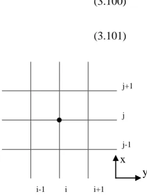
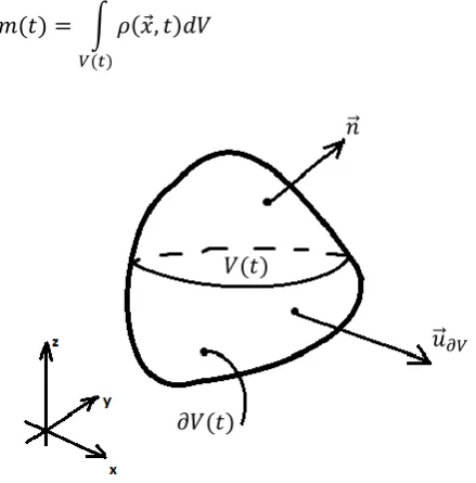
The continuity equation describes the conservation of mass. We will start with the definition of the mass within a control volume :

∫ ⃗

(2.1)

Figure 2.1 Schematic view of control volume

𝑛 ⃗

𝑢 ⃗_𝜕𝑉

(12)

(13)

(14)

⃗ ⃗ ⃗ ⃗ ̿ (2.17) Both terms can be rewritten. First we will use the chain rule of differentiations to transform the first term:

⃗ ⃗ ⃗ [ ⃗ ⃗ ] ⃗ ( ⃗ ⃗) ⃗ ⃗ ⃗ (2.18)

̿ ̿ ⃗ ̿ (2.19)

For a Newtonian fluid, the viscous stress tensor holds:

̿ [ ⃗ ⃗ ( ⃗ ⃗ ) ] [ ⃗ ⃗ ] ̿ (2.20) For incompressible flow [ ⃗ ⃗ ] . Furthermore for incompressible flow and , equation (2.18) transforms in:

̿ ⃗ ̿ ̿ ( ⃗ ⃗) ⃗ (2.21)

This leads to the following representation of the Navier-Stokes equation:

( ⃗ ⃗) ⃗ ⃗ ( ⃗ ⃗) ⃗ ⃗ (2.22) Now we expand the equation for and dividing it by :

𝒊=1

( )

(2.23) 𝒊=2

( )

Before continuing with the derivation of the boundary layer equations, we need to discuss another important assumption. This assumption is that the boundary layer is very thin in comparison with the length of the body. That is

(2.24)

Figure 2.2 Schematic view of flat plate with boundary layer[2]

This important assumption reduces the Navier-Stokes equations yet again. Prandtl used the concept of dimensional analysis from which he found the similarity parameters. Similarity parameters are used for flows for which streamline patterns are geometrically similar and distributions of dimensionless forces, temperatures and velocities are the same when plotted against nondimensional coordinates. That is the case in this particular problem. Let us introduce the following dimensionless variables:

(2.25)

(15)

(16)

( ) (2.36)

(2.37)

The result for the y-component of the momentum equation tells us that the pressure gradient in vertical direction is zero, so the pressure in vertical direction in the boundary layer is constant. This also tells us that the pressure on the outer edge of the boundary layer is imposed directly to the surface of the body.

(2.38)

Now we have the boundary layer equations for a flat plate at angle of attack of zero incidence in 2D steady, incompressible flow without effects of gravity or other volumetric forces.

( )

(2.39)

The above equations are subjected to the boundary conditions at the solid surface, i.e. the no-slip condition. The no-slip condition implies that there is no velocity in the x- and y-direction at the surface of the body. Furthermore at the edge of the boundary layer the velocity in x-direction is the identical to the free stream velocity in front of the plate. So the three boundary conditions are:

(2.40)

Note that due to the last boundary condition and the fact that at the edge of the boundary layer the change of velocity in y-direction is zero, i.e. , the x-component of the momentum equation applied at the edge of the boundary layer reduces to:

(17)

(18)

(3.10) This results in:

_(3.11)

For a similarity solution, equation (3.11) should be independent of . So this means that the power of x should be zero:

(3.12)

But there are two unknowns, so we need a second expression for P and Q in order to obtain the solution. For this we consider the boundary conditions, equation (2.40). The first boundary condition is . Substituting this with the new parameters:

(3.13)

A nor B will not be zero, this is a trivial solution. So this means that . The second boundary equation is . This results in:

(3.14) Since already, it follows that . The last boundary condition is . When we substitute this we obtain:

(3.15)

For the same reason at equation (3.12), we can state this boundary condition should be independent of x, so that:

(3.16)

We now have two equations - (3.12) and (3.16) - for P and Q. So we find:

(3.17)

We still need an expression for A and B. Considering equation (3.11) we choose for convenience:

(3.18)

And from equation (3.15) we set:

(3.19)

Equations (3.18) and (3.19) give us the opportunity to find the parameters A and B:

√ √ (3.20)

(19)

_√ _√

(3.21)

Note that and are dimensionless. The three boundary conditions required for the third-degree ordinary differential equation to solve are:

(3.22)

Let us look more closely to this result. We went from the partial differential equation of the x-momentum, equation (2.39), to an ordinary differential equation for . Since we found the stream function, we can use the definition of the stream function of equation (3.2) to obtain the velocity of the flow in x-direction :

(3.23)

For the velocity of the flow in y-direction it follows:

_(3.24)

This means that since the Blasius solution is only depending on , the velocity in x-direction depends on only. The vertical component of the velocity is a function of times a scaling factor proportional to .

3.1.2 Shooting method

To solve the Blasius equation, i.e. a third-order nonlinear ordinary differential equation, we rewrite the equation to three first-order ordinary differential equations. We then have three so-called initial value problems which can be solved. The Blasius equation is rewritten in such a way that it is an equation involving only a first-derivative:

(3.25)

(3.26)

(3.27)

The problem now is the missing third initial value . But since we know , we can use the shooting method. The shooting method is a procedure using a guess for the third, missing, initial value, carrying out the calculations and comparing the result with the result for which should be . To solve the initial value problem use is made of the Euler forward method. The goal of this technique is to approximate the first derivative in the differential equation. It is based on finding the next value of a graph by adding the old value plus the derivative of the curve at the old value times an arbitrary step size. This numerical method works well for small enough chosen step sizes. So Euler’s forward method for the three differential equations above results in:

(3.28)

(3.29)

(20)

3.1.3 Results

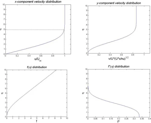
3.1.3.1 Velocity profile for flat plate

Using the guess for we can evaluate the three equations above and repeat this for up to large values of until does not change anymore. After this we check whether the result of the Euler forward method for high values of gives . If not, we choose another value for , repeat the calculations etc.. Using the shooting method we find:

(3.31)

The solutions for the components of the dimensionless velocity components in x- and y-direction are plotted in figure 3.1 and so are the functions and . Consider the plot of which corresponds to the distribution of the dimensionless x-component of the velocity; is dependent on and . So at two different -positions along the flat plate the velocity profile is the same. This means that in order to have the same value of , needs to compensate the change in . So along the plate the boundary layer will grow in vertical direction due to the increasing in such a way that the distribution remains identical in terms of . Such a result is called a self-similar solution.

(21)

(22)

( ) (3.38)

So the skin friction coefficient decreases as ( ) with increasing distance from the leading edge. For the skin friction coefficient of the entire plate we use the following equation:

∫ √

∫

(3.39)

This shows that with increasing the skin friction coefficient of the plate decreases.

3.1.3.4 Displacement thickness

This frequently used boundary layer property describes the difference between the case with hypothetical flow over a flat plate without a boundary layer and the actual flow with a boundary layer.

Figure 3.1 Schematic view explaining the influence of the boundary layer on external streamlines [2]

Because of the presence of a boundary layer, the streamlines passing through point are deflected upward over a distance . We can calculate this distance by equating the mass flow between the solid surface and the external streamline at point 1:

̇ ∫ (3.40)

And similarly at point 2:

̇ ∫ (3.41)

The mass flow through the surface at point 1 and through the surface at point 2 are equal since the streamline passes from point 1 to point 2. This means:

∫ ∫ (3.42)

We obtain from this equation the displacement thickness :

∫ ∫ ( ) (3.43)

(23)

∫ ( ) (3.44) We can transform this equation in terms of the transformed variables and from equation (3.21) and (3.23). This results in:

√

√ (3.45)

(3.46)

Substituting this in equation (3.44), results in:

√ ∫ ( )

( )

√ (3.47)

When we consider the numerical result of , we see that for all values above the result is 1.727. So when we reach the point of the edge of the boundary layer . This results in an equation for the displacement thickness:

( ) (3.48)

We see that also the displacement thickness is proportional to the square root of the x-position. This agrees with the definition of the displacement thickness, it is impossible to have a growing boundary layer and a decreasing displacement thickness. Now we can express the boundary layer thickness in terms of the displacement thickness:

√

(3.49)

This result tells us that the displacement thickness is about 3 times smaller than the boundary layer thickness itself.

3.1.3.5 Momentum Thickness

Another frequently used characteristic of a boundary layer is the momentum thickness. This property gives us an index proportional to the decrement of the flux of momentum due to the presence of the boundary layer. We will derive the momentum thickness with the help of figure 3.2.

(24)

We consider a mass flux across a segment of . Then consider the momentum flux (mass flux times the velocity) at segment with and without the presence of the boundary layer. First the momentum flux with the boundary layer:

(3.50)

And then without the boundary layer:

(3.51)

Integrating over the boundary layer, from and we obtain the total momentum flux. When we subtract equation (3.50) and (3.51) and take the integral, we obtain the total decrement in momentum flux:

̇ ∫ (3.52)

Now we assume that the missing momentum flux is the product of and the height , and compare these two definitions for the missing momentum flux due the presence of the boundary layer:

∫ (3.53)

We obtain from this equation the momentum thickness :

(∫ ) ∫ ( ) (3.54)

Again let us return to the situation where we have an incompressible flow ( and the velocity at the edge of the boundary layer is . Then the momentum thickness becomes:

∫ ( ) (3.55)

Also here we will use the similarity variables and from equation (3.21) and (3.23). This results in:

√ ∫ ( ) (3.56)

The equation in the integral ( ) cannot be integrated analytically. However, for will not change anymore and will be equal to 1.0. The numerical result of the integral is . So we obtain the momentum thickness in our case:

( ) (3.57)

So also the momentum thickness is proportional to ( ) . Therefore, also the momentum thickness grows with the square root of the x-position on the flat plate. The momentum thickness can be expressed in terms of the boundary-layer thickness and the displacement thickness:

(25)

(26)

(27)

(28)

(29)

(30)

( ) (3.98)

( ) (3.99)

∫

(31)

(32)

(33)

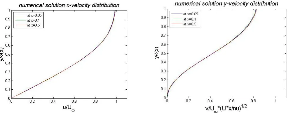
Figure 3.5 x- and y-component of the velocity in the boundary layer as function of of

We carried out these calculations for a flat plate of . The results are as expected; the solution is similar, independent of the x position. The second result we derive from this numerical approach is the skin-friction coefficient. By using a three-point formula using , we find the shear stress:

( )

) (3.112)

To find the skin-friction drag coefficient, we need to integrate this shear stress following equation (3.39). With the use of the trapezoidal rule we can carry out the integration. We find for the skin-friction drag coefficient:

√ (3.113)

(34)

(35)

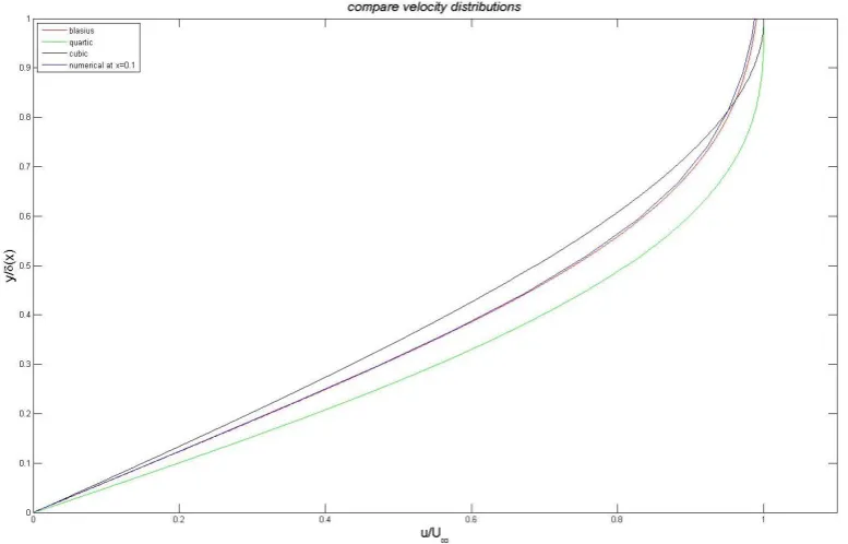
Figure 3.6 Comparison of Blasius’ velocity profile with velocity profiles computed using polynomial profiles and numerical method

We observe the failure of the polynomial approximation methods to represent the velocity profile of the Blasius solution. The cubic profile starts with a more accurate slope but fails the curvature near . The quartic profile starts too slow (or better, it has too high a speed close to the wall), but appears to match the exact solution more accurate near . The numerical solution shows a very similar velocity profile in comparison with Blasius’ solution. This is because in contrast with the approximation methods, the numerical approach has more degrees of freedom. That is the reason that the Blasius and numerical approach are not exactly the same, but agrees quite satisfactorily.

3.4.2 Skin friction coefficient

In contrast to the velocity profile, the skin friction drag coefficient of the numerical results is less accurate than the values obtained from the approximation methods based on the Integral Momentum Equation.

Blasius Cubic Quartic Numerical

√

(36)

Figure 3.7 Skin friction coefficient as function of x. The green curve is Blasius solution, the red curve the numerical solution

3.4.3 Boundary layer Thickness

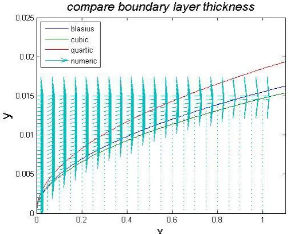
Also we consider the comparison of the boundary thickness obtained from the different approaches. With each method (analytical, approximation and numerical) we found solutions for the boundary layer thickness. With the use of the quiver function from Matlab, we can obtain a velocity plot for the numerical approach. We only show the velocity vectors for which , see figure 3.8:

Figure 3.8 Comparison of boundary layer thickness of Blasius’ solution with results from the Integral momentum equation and from the numerical solution

To look more closely, we will derive the boundary layer thickness at . For this comparison we take and _{, i.e.} _.

Blasius Cubic Quartic Numerical

(37)

(38)

(4.4)

4.1.2 Calibration of the Hot Wire

To measure the flow velocity with the Hot Wire, it is necessary to calibrate the probe. For making sure the manner in which calibration is carried out will not affect the measurements, the calibration is carried out in the wind tunnel itself. Also it is necessary to calibrate the probe at the same angle of attack as the angle of attack during the measurements. Bruun [9] describes that the angle of the probe influences the measurement. So the flow needs to come from the same direction as where the flow will come from when the wind tunnel is turned on. Using the funnel shown in the picture in figure 4.1 we are able to blow air in the direction of the probe. This funnel is connected with a device which can measure the pressure in terms of the heights of a water column, a Betz micro manometer. With this we can carefully set the speed of the flow from the funnel and we can calibrate the Hot Wire. Calibration and measurements are executed with the program Streamware Pro V5.02.

Figure 4.1 left: Betz manometer Right: Funnel with probe for calibration

It is also important to calibrate the position of the probe, since the position in the boundary layer influences the velocity. This is carried out with a broken Hot Wire and a multimeter. The multimeter is attached to the surface of the plate (which is of metal) and the ground of the probe. When the broken probe touches the surface, a current will flow which we can measure with the multimeter. Since we suppose that this position is the same for all individual probes, this gives a measure for the position of the probe with respect to the surface of the flat plate. In the discussion of the experiment we will discuss that this method has significant limitations. With this technique we obtain the first data point at a height of with respect to the surface of the plate.

4.1.3 Flap

(39)

(40)

Figure 4.4 Measured velocity distributions at x=0.095 m

(41)

4.2.2 With Flap

The second measurements has been carried out for the flat plate with the flap attached to the trailing edge. The flap is set at an angle of , in order to have the same pressures on both sides of the leading edge of the plate. Again, free stream velocities of and are used in the experiments. The results are presented in figure 4.6.

Figure 4.6 Comparison experimental velocity distributions for the flat plate with flap

Here we observe more agreements between the results for the two free stream velocities. Since the flap ensures equal pressures on both sides of the leading edge of the flat plate, the graphs should be similar to each other. Still there are some derivations between both graphs. This can be the cause of failures in the measurements. To find out if the measured dimensionless velocities agree, more experiments should be carried out.

4.3 Comparison of data

4.3.1 Comparison data with and without flap

(42)

Figure 4.7 Comparison experimental velocity distribution with and without flap

Indeed, the velocity distributions are higher for the experiments with the flap than the experiments without the flap.

4.3.2 Comparison experimental data with theory

Now we can compare the data from the experiments with the results from theory described in chapter 3. We only plot the data from the experiments with the flap and we compare this with the Blasius’ solution. The results are presented in figure 4.8.

Figure 4.8 Compare experiment with theory

(43)

The results can also be presented in another way. We now take the y-axis in a similar way as for the Blasius solution, i.e. as . Then we compare the Blasius solution with the data from the experiment with the flap for the free stream velocity of .

Figure 4.8 Comparison Blasius’ velocity profile with the measured data from

This graph confirms the conclusions, that the Hot Wire is capable to measure the velocity in the laminar boundary layer properly. This, because we observe a close similarity between Blasius’ solution and the data for a free stream velocity of . Same procedure is done for the measurement for a free stream velocity of . This graph is not put in this report since the figure shows great agreements with figure 4.8 and therefore also confirms the conclusion that the Hot Wire seems to be capable to measure the velocity in the laminar boundary layer properly.

4.3 Discussion

Some procedures had certain difficulties which we will discuss here. A major flaw in the experiment is the calibration of the position of the probe.

We used a broken Hot Wire in order to find the location of the probe with respect to the surface of the plate. This is carried out with a broken probe since Hot Wires are fragile and are likely to break when touching the surface of the plate. Here we assume that for every probe and for every measurement the location of the surface of the plate is the same. But since we are working in the very small region of the boundary layer ( , differences of tens of millimetres will affact the measurement significantly. Since the data from the experiments with the flap attached to the trailing edge did not match the solution of Blasius, we presume a failure of positioning the Hot Wire. Therefore we measured the location of the surface of the plate with three different broken Hot Wires. Before every measurement the probe was taken out of the probe support. The results are presented in figure 4.9. The probe was turned for measurements 6 to 10.

Figure 4.9 Height measurements with different Hot Wires

measurement 1 2 3 4 5 mean 6 7 8 9 10 mean

Probe 1 (mm) 4.34 4.39 4.43 4.41 4.31 4.38 5.29 5.31 5.33 5.28 5.29 5.30

Probe 2 (mm) 4.91 4.98 5.02 4.95 4.92 4.96 5.15 5.18 5.27 5.19 5.21 5.20

(44)

These results show differences in the position of the surface of the plate for different probes but also variations within the results for each probe itself. It also shows that the measurement of the height changes when the probe is turned . Where the average height for probe 2 and 3 differ when turning the Hot Wire, for probe 1 the difference is almost . It can be concluded that probe 1 is bent and therefore we cannot use this probe for calibrating the position of the surface of the plate. So in order to determine the height of the surface we only use probe 2 and 3. Since the heights vary for each probe it is not possible to determine the height within a margin less than . Therefore the height that is used in the presentation of the results is most likely not accurate. With this knowledge, we can fit the results from the experiments with Blasius’ solution. What we mean by this is we set the position of our first measured data point with a certain measured velocity equal to the corresponding height for this velocity from Blasius’ solution. With this we can investigate the measurement follow the curve from the Blasius euation. The graph was fitted with the first data point height of , a difference of with measured position. The results of fitting the experimental data with the Blasius solution is presented in figure 4.10.

Figure 4.10 Fitting experimental data with Blasius’ solution

This result shows satisfactory agreements with results from Blasius’ solution. Three factors can have contributed to this difference in height. First factor can be the unequal lengths of the probes. A slight difference in length of the Hot Wire probes can already contribute substantial to the deviation. Second factor can be the design of the probe holder. The probe is placed in the probe holder like a plug in a socket. The probe can twist slightly in the probe holder. But since we are searching for differences in the range of hundredths of millimetres, this can play a role. Third factor is the wing profile to which the probe holder is attached. This wing can also move slightly. This can also play a role in the deviation of the height of the surface.

Let us secondly discuss the use of the Betz micro manometer. We set the Betz manometer at a particular pressure to obtain a chosen flow velocity. At low speeds ( ) the pressure is not varying much, so it is difficult to set the right velocity. Furthermore, it is difficult to read off the pressure precisely. Fluctuations in the use of the Betz manometer give flaws in the calibration of the Hot Wire and therefore in the measurements.

4.4 Conclusions

(45)

(46)

(47)

5 Conclusions and Recommendations

5.1 Main Conclusions

In the present study analytical, numerical and experimental data has been obtained and analysed concerning the laminar boundary layer over a flat plate at zero degree incidence. In figure 3.6 the comparison between Blasius’ solution, the Integral Momentum equation based on von Karman’s integral momentum method and the numerical approach is presented. It is clear that the numerical approach produces a velocity distribution that compares very well with Blasius’ solution. This numerical approach can be used in situations for which analytical results are not available.

Experiments in the wind tunnel showed that Hot Wire Anemometry measurements are able to fit Blasius’ solution. This fitting is presented in figure 4.10. With the use of the flap at the trailing edge, we were able to vary the stagnation point at the leading edge such that the experiments could be compared properly with the theory. Due to the limitations of positioning the probe accurately, we cannot draw the conclusion that the Hot Wire is able to measure the velocity distribution in the boundary layer. However, we can conclude that the results of the measurements with the Hot Wire fit to Blasius’ solution and therefore it is expected that in the case of more accurate positioning of the probe, the Hot Wire is able to measure the velocity distribution within the boundary layer.

5.2 Recommendations

The most important limitation of this experiment was the positioning of the probe with respect to the surface of the flat plate. On one hand the Hot Wire is very fragile and may not touch the wall, on the other hand the laminar boundary layer was less than thick. Since we are working in this thin boundary layer, a difference in position of only a tenth of a millimetre has a significant impact on the results. In section 4.3 we discussed the used method to position the probe and the shortcomings of this method. We will discuss a number of suggestions for improving positioning of the probe.

There are two ways for to position the probe more accurate. First way is to look for a Hot Wire where its lengths are known with small margins of error. In this case, the probe support should be fixed more firmly. With these two conditions, we can calibrate the position of the probe with less margin of error. When these probes are not available, we should find another method to determine the height of the probe with respect to the surface of the plate. Since the probe is so fragile, we should either calibrate the probe contactless or make contact with the surface such that the probe will not break. A specially designed magnetic cube could be mounted to the wall. It should be magnetic to attach it to the wall. This cube has at a specific height a hole of diameter less than from which air is flowing. With the Hot Wire, we can detect the location of this flow and then the position of the probe is at a certain distance from the wall of the plate. This is positioning the probe contactless. Another option is to develop a probe support with some sort of antenna. The antenna can touch the wall to measure the height of the probe to the wall. The difference between the height of the antenna and the probe itself should then be measured, possibly using lasers.

(48)

(49)

6 References

1. Young, A.D., Boundary layers. AIAA education series 1989, Washington, DC: American Institute of Aeronautics and Astronautics : BSP Professional Books. xvii, 269 p.

2. Anderson, J.D., Fundamentals of aerodynamics. 4th ed. McGraw-Hill series in aeronautical and aerospace engineering 2007, Boston: McGraw-Hill Higher Education. xxiv, 1008 p. 3. Çengel, Y.A., Heat & Mass Transfer: A Practical Approach2007: McGraw-Hill Education

(India) Pvt Limited.

4. Schlichting, H. and K. Gersten, Boundary-layer theory. 8th rev. and enl. ed2000, Berlin ; New York: Springer. xxiii, 799 p.

5. Schobeiri, M., Fluid mechanics for engineers : a graduate textbook 2010, Berlin: Springer. xxi, 504 p.

6. Schetz, J.A., Boundary layer analysis 1993, Englewood Cliffs, N.J.: Prentice Hall. xxii, 586 p. 7. Dynamics, D., Probes for Hot-wire Anemometry, N. Instruments, Editor 2012. p. 25.

8. Durst, F., E.S. Zanoun, and M. Pashtrapanska, In situ calibration of hot wires close to highly heat-conducting walls. Experiments in Fluids, 2001. 31(1): p. 103-110.