1521
Assessing Quality Estimation Models for Sentence-Level Prediction
Hoang Cuong and Jia Xu
Cuny University of New York
Abstract
This paper provides an evaluation of a wide range of advanced sentence-level Quality Estimation models, includingSupport Vector Regression,Ride Regression,Neural Networks,Gaussian Pro-cesses,Bayesian Neural Networks,Deep Kernel LearningandDeep Gaussian Processes. Beside the accurateness, our main concerns are also the robustness of Quality Estimation models. Our work raises the difficulty in building strong models. Specifically, we show that Quality Estima-tion models often behave differently in Quality EstimaEstima-tion feature space, depending on whether the scale of feature space is small, medium or large. We also show that Quality Estimation mod-els often behave differently in evaluation settings, depending on whether test data come from the same domain as the training data or not. Our work suggests several strong candidates to use in different circumstances.
1 Introduction
Quality Estimation (QE) (Blatz et al., 2004; Specia et al., 2009) is an important topic in Natural Language Processing (NLP). QE aims to predict the quality of Machine Translation (MT) outputs without human references. QE has a lot of potential. Such a case is automatically optimizing MT systems without having reference of translation outputs. Another example is MT for gisting by users of online translation systems. QE can also reduce post-editing human effort in disruptive ways. As most QE research has conducted at sentence level, we focus on the sentence level in this study.
Prior work developed strong QE predictors by creating powerful QE features. Hand-craft and syn-tactic feature templates have been proposed for a while (e.g. see Specia et al. (2009) and Martins et al. (2017)). The representation of words, phrases and sentences can also be learned automatically using Neural Networks, serving as powerful QE features (Kreutzer et al., 2015; Shah et al., 2015b; Kim and Lee, 2016; Kim et al., 2017; Chen et al., 2017; Bic¸ici, 2017; Martins et al., 2017).
Meanwhile, using a relevant QE model is also very important in QE. Various QE models have been applied in different QE settings, such asSupport Vector Regression(Cortes and Vapnik, 1995; Specia et al., 2009),Ride Regression(Hoerl and Kennard, 2000; Wisniewski et al., 2013),Neural Networks(NNs) (Avramidis, 2017; Paetzold and Specia, 2016; Paetzold and Specia, 2017) andGaussian Processes(GPs) (Rasmussen and Williams, 2005; Cohn and Specia, 2013).
Given that there are many powerful regression models, it is tempting to have an understanding of which sentence-level QE models we should use. Prior work has been attempted to provide an answer (e.g. see Cohn and Specia (2013), Soricut et al. (2012), Wisniewski et al. (2013), and Beck et al. (2016)). However, the assessment of QE models is often limited in the number of QE features. For instance, Cohn and Specia (2013) conduct experiments with only17 QE features. Also, the assessment is in only the
Standardsetting (i.e. test data come from the same domain as training data), which is often violated in practice.
Interesting and important questions are still open to date. For instance, given different scale of feature space, it is not clear which QE models we should use and how to build them properly (e.g. howdeep
a NN we should use). Given different training/test settings, it is also not clear which models produce more robust QE performance than others.1 Specifically, we are interested in bothStandardandDomain Adaptation(DA) settings (i.e. test data come from a different domain to the training data). We also focus onKnowledge Transfer(KT) setting (i.e. QE model is trained on a dataset from a specific language pair but the model is tested on a test set with a different language pair).
This work provides an evaluation of a wide range of QE models and settings as the main contribution. Not only assessing popular QE models, we also propose to use several novel models for QE including
Bayesian Neural Networks(Neal, 1996),Deep Kernel Learning(Wilson et al., 2016b),Deep Gaussian Processes(Damianou and Lawrence, 2013). Our results also raise concern about overfitting in applying QE models in different settings. We also show how complex the interactions are between QE features. Meanwhile, we also show that our proposed models work very well in certain circumstances.
In detail, we summarize the most interesting findings as follows. First, Support Vector Regression, despite being considered a strong QE model, is far from achieving top performance. It also provides a rather weak performance in DA and KT setting. Meanwhile, our experiments show that the QE feature space is highly complex. Specifically, we show that while the feature space could be large, most of the features in the space are usually useful so that applying sparse QE models is often less effective than non-sparse QE models.
Second, a shallow NN seems to gain a strong performance in the Standard setting. This is interesting, as previous attempt to use shallow NNs for QE (e.g. see Avramidis (2017)) failed to deliver a competitive result in the standard WMT setting (see Bojar et al. (2017) for a reference). Perhaps, their network parameter settings are not good enough to make the model work. We also attempt to use deep NNs for QE, and show that they do not contribute a better performance in the Standard setting. This is because training deep NNs for QE requires lots of labeled data to control the risk of overfitting.
Increasing the number of units in the hidden layer larger could degrade the performance. Specifically, we show that training a large NN could be overfitting, and available QE datasets are not large enough to reduce the risk. But can we still make a very large NN work for QE? This paper shows that we can do so by using Gaussian Processes (GPs).
We investigate GPs from the viewpoint of a non-parametric version of shallow NNs, and analyze their advantages over NNs: GP has an infinite number of hidden units in the hidden layer, GP has a built-in feature weighting mechanism and model is more robust to over-fitting. We also analyze their disadvantages, showing the cases where GPs completely fail to deliver good results. Finally, we also propose a solution to address their drawbacks.
Third, we observe a very weak performance of NNs in the DA and KT setting. While we are aware of concerns of applying NNs to different domains in other NLP tasks (e.g. Machine Translation (Koehn and Knowles, 2017) and Sentiment Analysis (Radford et al., 2017)), this is the first study to raise this issue in QE. We propose three methods that make NNs work well with the challenging setting.
First, we propose to use deep NNs for QE to DA and KT settings. We attribute this observation to the fact that deep NNs learn high-level (instead of low-level) features, which may work well across domains/datasets. Second, we propose to use GPs under these conditions because of their robustness.
These models, however, work well only when we train them with a small set of features. We then propose to use a combination of the two, a.k.a Deep Kernel Learning, to address the problem. For this deep model, the GP is put on top of a NN, aiming to combine the best of both worlds. We show that it provides an even stronger performance.
Third, we propose to use Bayesian NNs to the DA and KT setting. It is a type of neural networks with a prior distribution on its weights. The common perception is that it is hard to apply the model to NLP because of its difficulty in training. This paper shows that it is not the case, thanks to recent advances in Variation Inference (with stochastic variational inference (Hoffman et al., 2013), black-box variational inference (Ranganath et al., 2014) and the reparameterization trick (Kingma and Welling, 2014; Rezende et al., 2014)). We show that Bayesian NNs provide another powerful solution to the problem.
1We should note that we focus on the accurateness and robustness of QE models. However, calculation cost is not considered
2 Related Work
Developing different regression QE model at sentence-level has been one of the main focuses in QE.
Support Vector Regression is perhaps the most popular QE sentence-level model (Specia et al., 2009; Soricut et al., 2012; Kozlova et al., 2016). Gaussian Processes(GPs) (Cohn and Specia, 2013; Shah et al., 2013; Beck et al., 2015; Beck et al., 2016) andRide Regression(Wisniewski et al., 2013) are also popular models in QE. NNs have been widely deployed as a non-linear classification model in QE (e.g. see Blatz et al. (2004), Espl`a-Gomis et al. (2015) and Espl`a-Gomis et al. (2016)). Recently, NNs have also been attempted to use as a regression QE model at sentence-level (Avramidis, 2017; Paetzold and Specia, 2016; Paetzold and Specia, 2017). Other less popular models are proposed, e.g. Regression Trees (Soricut et al., 2012; Wisniewski et al., 2013), Extremely Randomized Trees (Negri et al., 2014).
Given different QE models, it is tempting to have an understanding of which QE models we should use. There have been several attempts to answer this important question (e.g. (Cohn and Specia, 2013; Soricut et al., 2012; Wisniewski et al., 2013; Beck et al., 2016)). For instance, Cohn and Specia (2013) and Beck et al. (2015) show that choosing a model between GPs and SVR could make a difference. Meanwhile, Avramidis (2017) compares NNs with SVM. The comparison, however, limits in only a specific pair of models (e.g. GPs-SVR and SVR-NNs). Experiments are also with only medium-size feature space (17 features) and in the Standard setting. We extend the work extensively in regards to having a larger number of QE models, and having a systematic manner with different settings (testing with different feature space, different training/test settings). Moreover, our results not only provide a better understanding in regards to QE Models for sentence-level prediction, but also raise concern about overfitting in applying QE models in different settings.
Our work also puts attention to the setting where test data comes from different distributions or do-mains to the training/dev data (i.e. DA and KT). We share the same views with the work of R´ıos and Sharoff (2016), Shah and Specia (2016), de Souza et al. (2014a), de Souza et al. (2014b) and de Souza et al. (2015) in regards to this setting. Specifically, we believe utilizing a dataset from one specific dis-tribution/domain to use for other disdis-tribution/domain is very useful. The related studies focus on using multiple task learning (Shah and Specia, 2016; de Souza et al., 2014a), or utilizing unlabeled data (R´ıos and Sharoff, 2016) to address the problem. Meanwhile, our work focuses on assessing the robustness of QE models to improve model performance in this setting.
Prior work revealed that the interactions between QE features are non-linear (e.g. see Shah et al. (2015a)). We extend the result in the sense that we show the interactions are not only non-linear but also highly complex. However, we show that we do not need a non-stationary function to model the relationship (i.e. whether there is a jump discontinuity or an isolated tall peak).
A distant research line is feature selection. Specifically, Soricut et al. (2012) use a computationally intensive method to find all 224 possible combinations, from an initial set of 24 features to find the best combinations. Another distantly related work focuses on developing non-linear methods for feature selection in QE (Shah et al., 2015a). While the research line is distant to our study, we share the same views with the studies in that a complex combination of features, rather than a simple linear combination, may bring significant benefits to QE.
Our work also introduces Deep Kernel Learning, a hybrid NN with GPs, as a regression model to not only QE but also NLP for the first time. This combination model has been attempted recently in the Machine Learning community, pioneered by the work of Wilson et al. (2016a) and Al-Shedivat et al. (2017). Specifically, Wilson et al. (2016a) apply the framework toairlineandimageclassification. Al-Shedivat et al. (2017) apply the framework to different regression problems in Machine Learning. Recently, Bradshaw et al. (2017) also apply the framework to image classification andtransferlearning.
3 Models
approximate the inverse of the covariance matrix with the inverse of theM×M“pseudo matrix” instead. For this reason, we do not observe any problem with scaling GPs to QE datasets in our experiments. For our implementation, GPs are implemented in the standard GPflow, a Gaussian process library using TensorFlow (de G. Matthews et al., 2016).
3.3.2 Deep Gaussian Processes
This work will show that the relationship between the space of input features and corresponding output is non-linear and highly complex. A further question we asked is whether we need a non-stationary
function to model the relationship (i.e. whether there is a jump discontinuity or an isolated tall peak). One additional contribution of this work is to provide an understanding of this issue.
Specifically, we introduce another kind of deeper NNs for QE, namely Deep Gaussian Processes
(Damianou and Lawrence, 2013). Deep GPs combine GPs with deep architectures. Let us denote a GP model forY asY ∼GP(0, K(X, X)). Instead of having only a simple layer of GP, we can stack many more. This is mathematically equivalent to having the form:
Y ∼fL(fL−1(. . . f1(X, X). . .)), (3)
wherefl(·)∼GP(0, Kl(·,·)). Stacking many more layers helps the model able to learn to approximate non-stationary functions (e.g. see Damianou and Lawrence (2013) and Vafa (2016)).
Training the model is more complicate, but doable with recent advanced approximate methods (e.g. Approximate Expectation Propagation (Bui et al., 2016), Doubly Stochastic Variational Inference (Sal-imbeni and Deisenroth, 2017)). In this work we choose the work of Sal(Sal-imbeni and Deisenroth (2017) to train the model because of its simplicity and efficiency.
3.3.3 Deep Kernel Learning
In theory, GP with the SE kernel function is an universal approximator (Micchelli et al., 2006). Unfor-tunately, the representational power offered by the kernel can be very limited as the kernel is perhaps too simple. This may make it less effective when applying the model to a high dimensional QE feature space. It is not easy to address the problem.
In this work, we propose to use Deep Kernel Learning (DKL) to address the challenge. This type of network is a deep network: it has input layer, hidden layers, and a GP model on the top. The formulation for the model is thusY ∼GP(0, N N(X))instead ofY ∼GP(0, K(X, X)), whereN N(X)represents a NN instead of a simple kernel functionK(·,·). In our experiments, DKL is a shallow NN plus a GP model stacked on the top.
Technically, all GPs parts are differentiable (Rasmussen and Williams, 2005), including the Cholesky decomposition that computes the inverse of the M ×M “pseudo matrix”. For this reason, the model can be trained in an end-to-end fashion with back-propagation. Specifically, the model can be trained end-to-end using stochastic variational approach (Wilson et al., 2016a) or semi-stochastic block-gradient approach (Al-Shedivat et al., 2017). We choose the work of Al-Shedivat et al. (2017) to train the model because of its efficiency.
We propose to use DKL for QE because of two potential benefits. First, such a combination may work well with high dimensional input space since the flow goes from a NN to the GP layer. Second, it may be more robust because the model enjoys the robustness of GPs in general. Indeed, while deep NNs are found to be overfitting, DKLs are found to be very robust in our experiments.
3.3.4 Bayesian Neural Networks
Bayesian NNs are a type of NNs with a prior distribution on the weights. We introduce the model to QE because of their robustness.
Pre-dictive distribution of outputy∗ given a new inputx∗can be computed as follows:
p(y∗|x∗, X, Y) = Z
p(y∗|x∗,w)p(w|X, Y)dw.
p(w|X, Y) = p(w) QN
i=1p(yi|xi,w)
p(Y|X) .
Given a new inputx∗, Monte Carlo estimation can be used to get an unbiased estimate of it by sampling from the variational posterior
p(y∗|x∗, X, Y)' 1
M
M
X
i=1
p(y∗|x∗,wi). (4)
where eachwi is sampled fromp(w|X, Y). We use Bayesian NNs with50hidden units in our experi-ments. We found that using a larger number of units hurts the performance.
The model comes with a cost: it is non-trivial to compute the posterior distribution of network param-etersp(w|X, Y)because of the intractable marginal distributionp(Y|X). Variational Inference can be used to address the problem. It uses a variational distributionqθ(w) =QiL=1qθi(wi)to directly approx-imatep(w|X, Y). Eachqθi(wi)is basically a normal distribution paramaterized by mean and standard deviation:
qθi(wi) =N(wi|µi, δ2i) (5)
Training the model is efficient, thanks to stochastic variational inference (Hoffman et al., 2013) and the reparameterization trick (Kingma and Welling, 2014; Rezende et al., 2014)).
As a side note, our Bayesian NNs implementation is based on ZhuSuan, a well-developed framework for Bayesian Deep Learning (Shi et al., 2017).
4 Experiments Settings
Our training data is a collection of a pair of source/target sentences together with a HTER score (Snover et al., 2006) - the minimum edit distance between the machine translation and its manually post-edited version. All the datasets we conducted experiments in our study are standard WMT shared task datasets. The datasets are all publicly available. We also release our implementation for the code,3 making it available for reproducing results.
This work studies three different QE scenarios:
• Standard Setting: The test data comes from the same distribution as the training/validating data.
• Domain Adaptation Setting: The test data comes from a different distribution as the train-ing/validating data.
• Knowledge Transfer Setting: The test data comes from a different language pair as the train-ing/validating data.
Previous QE studies mainly focus on Standard setting. Our focus is also on DA setting, because we inevitably will come across data that is sampled from a different distribution to our training data when using QE models in the wild. Closely related to this is fine-tuning models on a new domain. However, we are interested in the aspect of NOT fine-tuning our models. This is because information of test data is not provided in advance when applying a QE model in the wild.
We are also interested in KT setting. Utilizing a dataset from one language pair to use for other language pairs is very useful, given that QE datasets are limited and language-specific.
Our experiments are with different feature sets. For medium-scale QE feature space, we use the standard17QE features (see Bojar et al. (2017)). For large-scale QE feature space, we enrich the feature
Model
Standard Setting Domain Adaptation Knowledge Transfer Train/Valid: Train/Valid: Train/Valid: WMT EN-DE 2016 WMT DE-EN 2017 WMT DE-ES 2015
EN-DE DE-EN Test: Test: Test:
WMT EN-DE 2017 WMT EN-DE 2017 WMT EN-DE 2017
Linear Model 23.48 29.47 − − −
Support Vector Regression 17.47 17.79 20.28 20.69 22.68 Kernel Ridge Regression 17.41 17.47 20.55 28.67 21.19 Shallow Neural Networks 17.46 17.15 20.81 24.96 23.46
Deep Neural Networks 17.51 17.32 19.45 22.85 20.51
Gaussian Processes 17.39 17.05 20.23 21.03 21.12
Deep Gaussian Processes 17.70 17.36 20.20 22.46 21.15
Deep Kernel Learning 17.35 17.28 19.68 21.93 19.93
Bayesian Neural Networks 17.57 17.76 20.65 21.64 23.77 Deep Bayesian Neural Networks 18.44 18.34 18.83 21.19 20.23
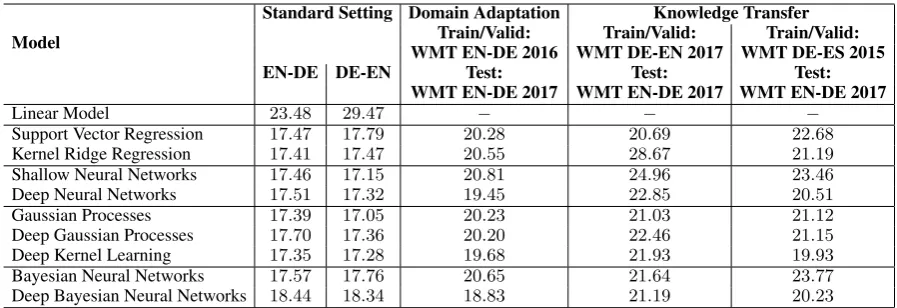
Table 1: Assessing QE Models for Sentence-Level Prediction (Medium-scale QE feature space).
set using unsupervised learning. Specifically, we trained a multiplicative LSTM (Krause et al., 2017) with4,096units on a very large publicEnglishcorpus (see McAuley et al. (2015)) to predict the next character for a string. These4,096units are found to be meaningful in NLP tasks in general such as Sentiment Analysis (Radford et al., 2017). This work shows that they are very useful to QE as well. While we can add all units as extra features, this turns out to be expensive. We rather use only arandom
subset of them (53and123units). In the end, our large-scale QE feature space experiments are with two feature sets with70and140features respectively.4
5 Standard Setting
We first present results with WMT QE 2017 shared task (EN-DE and DE-EN). There are various eval-uation metrics that are often used in Quality Estimation, including Pearson’s correlation, Mean Average Error and standard Root Mean Squared Error. Because of space constraints, we report only root-mean-square error (RMSE):
RM SE = s
PN
1 (HT ERref −HT ERpred)2
N ∗100, (6)
whereN is the size of test data. Meanwhile, we emphasize that the important findings in our work are consistent with the other metrics.
5.1 Medium-scale setting
Table 1 presents the result with medium-scale QE feature space. We detail most important findings. First, in this setting, we do not observe important advantages of using different models. There is not a clear winner, and the difference between the best model and other top models is quitemarginal. As a site note, SVR is far from achieving top performance (e.g. 17.79vs17.01for WMT QE DE-EN 2017 task). Meanwhile, Table 1 reveals that the relationship between the space of input features and corresponding output is fully non-linear. Specifically, having a linear QE model provides a far suboptimal performance (e.g. 23.48 with EN-DE), compared to other complex models (e.g. Deep Kernel Learning: 17.35. We also do not observe any significant improvement by using SVR instead of KRR. The fact that a sparse model (SVR) does not help over a non-sparse model (KRR) indicates most features are useful. Combining with the fact that the feature space is non-linear, the QE feature space seems highly complex. Shallow NNs with512units produce a competitive result. This is interesting, as previous attempt to use shallow NNs for QE (e.g. see Avramidis (2017)) failed to deliver a competitive result in the standard WMT setting (see Bojar et al. (2017) for a reference). Perhaps, their network parameter settings are not good enough to make the model work. For the sake of completeness, our network parameter setting is
4Surprisingly, we found that training a good QE model only with the set of53or123extra features improves the performance
as follows. The models were regularized with dropout (Srivastava et al., 2014) with rate0.5and were trained with Adam (Kingma and Ba, 2014) with rate0.0001.
Meanwhile, Bayesian NNs do not shine with this setting. Given that Bayesian NNs are suitable to the scenario of having little training data, we conclude that the quantity of being “little” should be much smaller than our QE training data. (Our training data are with around10K-20Ksentences.) Deep NNs and deep Bayesian NNs do not help much with Standard setting. Table 2 presents results with other settings of hidden layers for deep NNs.
DNNs EN-DE DE-EN NNs EN-DE DE-EN DGPs DE-EN GPs DE-EN EN-DE
1 Layer 17.46 17.15 512 17.46 17.15 1 Layer 17.01 w. FW 17.36 17.01 2 Layers 17.47 17.26 1024 17.44 17.14 2 Layers 17.28 w.o. FW 17.72 17.56 3 Layers 17.51 17.29 16384 17.51 17.34 3 Layers 17.36
4 Layers 17.48 17.37 32768 17.40 17.32 4 Layers 17.22 5 Layers 17.54 17.35 Infinite (GP) 17.36 17.05 5 Layers 17.34
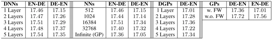
Table 2: Detailed analyses with different models in the Medium-scale setting. Specifically, using deep NNs (DNNs) does not help much. Using large NNs improves the performance, but only if the model is robust in training (i.e. as in GPs). It is also unlikely to need a QE model that is capable of approximating non-stationary functions, as we found deep GPs (DGPs) does not gain any significant improvements. Finally, feature weighting (F.W.) mechanism in GPs is also important. Turning it off rather gives worse results.
GPs are competitive with Standard setting and medium-scale QE feature space. We recall that GP is a non-parametric version of a shallow NN with an infinite number of units in the hidden layer (Neal, 1996). Detail analyses confirm that it is a good fit to medium-scale QE feature space because of the following reasons. First, having a substantially larger number of hidden units may help. However, we notice that having a larger NN may not improve performance, as in Table 2. That is, it helps only the case when the model is robust in training, as in GPs.
Second, most features in the feature space are useful. However, each of them should have a certain degree of relevance to the task. GPs can capture this. As in Eq 1, ifλdis larger, then thedthfeature is less important. Meanwhile, a smallλdindicates that the feature is crucial to the task. To this end, we noticed that their values are different in our experiments, and neither of them are too large or too small. We also noticed that once we use only a single hyper-parameterλfor all the features, we observe a significant drop in performance, as shown in Table 2. This confirms that the feature weighting mechanism is also important in GPs.
Meanwhile, deep GPs do not provide any improvement over GPs. We provide detailed statistics with other configurations of deep layers in Table 2. It is therefore unlikely to need a QE model that is capable of approximating non-stationary functions. In other words, the relationship between the space of input features and corresponding output is unlikely to have jump discontinuities or isolated tall peaks.
5.2 Large-scale setting
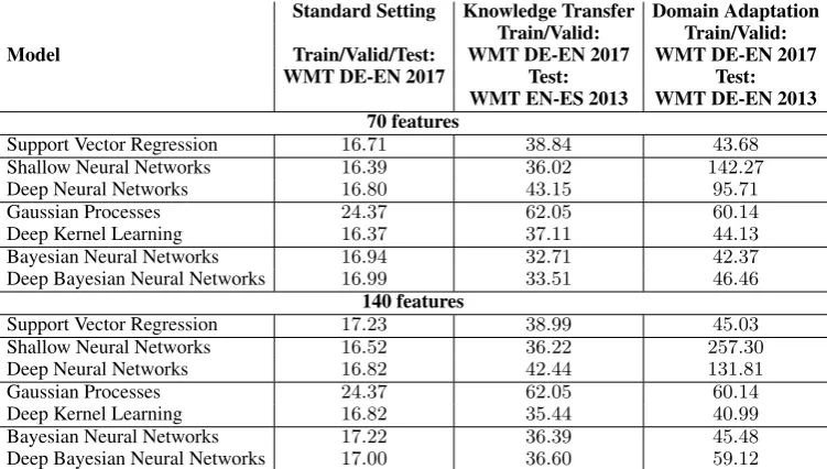
We now turn our attention to large-scale setting.5 Table 3 presents the result in detail. Here, we do not report KRR and Deep GPs because they seem not to be a right model for QE.6
The three most important observations are as follows. First, it is surprising to see that there is also not a clear winner, and the difference between the best model and other top models is also quitemarginal. Second, GPs do not provide competitive results with this setting. This is because simple SE kernel function is not representative enough to learn the similarity in high-dimensional QE feature space. We also tried other advanced kernel functions, such as Matern kernel (Rasmussen and Williams, 2005), Polynomial kernel (Rasmussen and Williams, 2005), mixture of SE kernels (Wilson and Adams, 2013) and Additive Kernels (Duvenaud et al., 2011) without success.
5
We report the Standard setting for large-scale experiments only for DE-EN. Specifically, the pretrained LSTM model is made available athttps://github.com/openai/generating-reviews-discovering-sentimentby Radford et al. (2017). Our large-scale feature experiments are thus reproducible.
to the fact that deep NNs learn high-level features, which may work well across domains/datasets. Un-fortunately, this seems to be only the case with medium-scale QE feature space. With large-scale setting deep NNs produce a suboptimal performance. It is indeed non-trivial to train deep NNs with the settings given small training data we have. Deep NNs also often produce HTER scores that are outside the range of[0:1]with these settings.
Third, using GPs for QE gains robust performance across various medium-scale QE feature space adaptation/knowledge transfer tasks. Unfortunately, this is not the case with large-scale setting.
Using Bayesian NNs and DKL provides a powerful solution to the DA and KT setting. Robustness is the key to their success under these settings. As a side note, deep Bayesian NNs provide good solution to DA and KT setting only with medium-scale setting.
Finally, our work shows if we choose a right QE model to apply in the wild, the QE prediction is robust. For instance, the performance of using deep NNs, DKL and deep Bayesian NNs is still very promising (19.45,19.68and18.83respectively) when they are trained with WMT EN-DE 2016 dataset but tested with WMT EN-DE 2017 test data.
Moreover, our results show that it is promising to utilize a QE dataset from one language pair to use for other language pairs. Let us present our good results with the WMT QE 2017 EN-DE test set as an example. Our result with DKL trained with WMT DE-ES 2015 is19.93while the best QE model trained on the in-domain training/validating data is17.35.
Our work also raises the challenge of building a better QE model with a large feature set. As in Table 3, model performance is often far from being robust/accurate across different domains/datasets.
7 Conclusion
This paper contributes a significant amount of efforts of assessing advanced sentence-level QE models. We show that having powerful features is not enough, as we also need a right model to use. We recom-mend to use shallow NNs with Standard setting, but we do NOT recomrecom-mend deep NNs with this setting. When it comes to medium-scale QE feature space, we recommend using GPs.
Meanwhile, we observe a very weak performance of NNs when applying the model in the wild (i.e. Adaptation and Knowledge Transfer setting). GPs model is a right option in these cases, but only with medium-scale setting. Bayesian NNs work well for both DA and KT settings, but not Standard setting.
Each model works well in certain circumstances. There is an exception, though, with Deep Kernel Learning. We found that the QE model is a strong candidate to use in real-world scenario.
Acknowledgements
We would like to thank reviewers for their insightful comments on the paper. This research was partially supported by National Science Foundation (NSF) Award No. 1747728 and National Science Foundation of China (NSFC) Award No. 61672524. We express our gratitude to the Provost office, the Dean’s office, the Department of Computer Science, and the Research Foundation of Hunter College at CUNY for partially funding our research.
References
Maruan Al-Shedivat, Andrew Gordon Wilson, Yunus Saatchi, Zhiting Hu, and Eric P. Xing. 2017. Learning scalable deep kernels with recurrent structure. https://arxiv.org/abs/1610.08936.
Eleftherios Avramidis. 2017. Sentence-level quality estimation by predicting hter as a multi-component metric. pages 534–539. Association for Computational Linguistics.
Daniel Beck, Trevor Cohn, Christian Hardmeier, and Lucia Specia. 2015. Learning structural kernels for natural language processing. Transactions of the Association for Computational Linguistics, 3:461–473.
Ergun Bic¸ici. 2017. Predicting translation performance with referential translation machines. InProceedings of
the Second Conference on Machine Translation, Volume 2: Shared Task Papers, pages 540–544, Copenhagen,
Denmark, September.
John Blatz, Erin Fitzgerald, George Foster, Simona Gandrabur, Cyril Goutte, Alex Kulesza, Alberto Sanchis, and Nicola Ueffing. 2004. Confidence estimation for machine translation. InProceedings of the 20th International
Conference on Computational Linguistics, COLING ’04.
Ondˇrej Bojar, Rajen Chatterjee, Christian Federmann, Yvette Graham, Barry Haddow, Shujian Huang, Matthias Huck, Philipp Koehn, Qun Liu, Varvara Logacheva, Christof Monz, Matteo Negri, Matt Post, Raphael Rubino, Lucia Specia, and Marco Turchi. 2017. Findings of the 2017 conference on machine translation (wmt17). In
Proceedings of the Second Conference on Machine Translation, Volume 2: Shared Task Papers, pages 169–214,
Copenhagen, Denmark, September.
John Bradshaw, Alexander G. de G. Matthews, and Zoubin Ghahramani. 2017. Adversarial examples, uncertainty, and transfer testing robustness in gaussian process hybrid deep networks. https://arxiv.org/abs/1707.02476.
Thang D. Bui, Jos´e Miguel Hern´andez-Lobato, Daniel Hern´andez-Lobato, Yingzhen Li, and Richard E. Turner. 2016. Deep gaussian processes for regression using approximate expectation propagation. InProceedings of
the 33rd International Conference on International Conference on Machine Learning - Volume 48, ICML’16,
pages 1472–1481. JMLR.org.
Zhiming Chen, Yiming Tan, Chenlin Zhang, Qingyu Xiang, Lilin Zhang, Maoxi Li, and Mingwen WANG. 2017. Improving machine translation quality estimation with neural network features. InProceedings of the Second
Conference on Machine Translation, Volume 2: Shared Task Papers, pages 551–555, Copenhagen, Denmark,
September.
Trevor Cohn and Lucia Specia. 2013. Modelling annotator bias with multi-task gaussian processes: An application to machine translation quality estimation. InACL (1), pages 32–42. The Association for Computer Linguistics.
Corinna Cortes and Vladimir Vapnik. 1995. Support-vector networks.Mach. Learn., 20(3):273–297, September.
Andreas C. Damianou and Neil D. Lawrence. 2013. Deep gaussian processes. InAISTATS, volume 31 ofJMLR
Workshop and Conference Proceedings, pages 207–215. JMLR.org.
Alexander G. de G. Matthews, Mark van der Wilk, Tom Nickson, Keisuke Fujii, Alexis Boukouvalas, Pablo Le´on-Villagr´a, Zoubin Ghahramani, and James Hensman. 2016. Gpflow: A gaussian process library using tensorflow. https://arxiv.org/abs/1705.08933.
Jos´e G. C. de Souza, Marco Turchi, and Matteo Negri. 2014a. Machine translation quality estimation across domains. InCOLING, pages 409–420. ACL.
Jos´e G. C. de Souza, Marco Turchi, and Matteo Negri. 2014b. Towards a combination of online and multitask learning for mt quality estimation: a preliminary study.
Jos´e Guilherme Camargo de Souza, Matteo Negri, Elisa Ricci, and Marco Turchi. 2015. Online multitask learn-ing for machine translation quality estimation. InACL (1), pages 219–228. The Association for Computer Linguistics.
David K Duvenaud, Hannes Nickisch, and Carl E. Rasmussen. 2011. Additive gaussian processes. InAdvances
in Neural Information Processing Systems 24, pages 226–234. Curran Associates, Inc.
Miquel Espl`a-Gomis, Felipe S´anchez-Mart´ınez, and Mikel L. Forcada. 2015. Using on-line available sources of bilingual information for word-level machine translation quality estimation. InProceedings of the 18th Annual
Conference of the European Association for Machine Translation, pages 19–26, Antalya, Turkey, May.
Miquel Espl`a-Gomis, Felipe S´anchez-Mart´ınez, and Mikel Forcada. 2016. Ualacant word-level and phrase-level machine translation quality estimation systems at wmt 2016. InProceedings of the First Conference on Machine
Translation: Volume 2, Shared Task Papers, pages 782–786. Association for Computational Linguistics.
Arthur E. Hoerl and Robert W. Kennard. 2000. Ridge regression: Biased estimation for nonorthogonal problems.
Technometrics, 42(1):80–86.
Matthew D. Hoffman, David M. Blei, Chong Wang, and John Paisley. 2013. Stochastic variational inference.
Journal of Machine Learning Research, 14:1303–1347.
Hyun Kim and Jong-Hyeok Lee. 2016. Recurrent neural network based translation quality estimation. In
Hyun Kim, Hun-Young Jung, Hong-Seok Kwon, Jong-Hyeok Lee, and Seung-Hoon Na. 2017. Predictor-estimator: Neural quality estimation based on target word prediction for machine translation. ACM Trans.
Asian & Low-Resource Lang. Inf. Process., 17(1):3:1–3:22.
Diederik P. Kingma and Jimmy Ba. 2014. Adam: A method for stochastic optimization.CoRR, abs/1412.6980.
Diederik P. Kingma and Max Welling. 2014. Auto-encoding variational bayes.ICLR, abs/1312.6114.
Philipp Koehn and Rebecca Knowles. 2017. Six challenges for neural machine translation. InProceedings of the
First Workshop on Neural Machine Translation, pages 28–39, Vancouver, August.
Anna Kozlova, Mariya Shmatova, and Anton Frolov. 2016. Ysda participation in the wmt’16 quality estimation shared task. InProceedings of the First Conference on Machine Translation, pages 793–799, Berlin, Germany, August. Association for Computational Linguistics.
Ben Krause, Liang Lu, Iain Murray, and Steve Renals. 2017. Multiplicative lstm for sequence modelling. https://arxiv.org/abs/1609.07959.
Julia Kreutzer, Shigehiko Schamoni, and Stefan Riezler. 2015. Quality estimation from scratch (quetch): Deep learning for word-level translation quality estimation.
Andr´e Martins, Marcin Junczys-Dowmunt, Fabio Kepler, Ram´on Astudillo, Chris Hokamp, and Roman Grund-kiewicz. 2017. Pushing the limits of translation quality estimation. Transactions of the Association for
Compu-tational Linguistics, 5:205–218.
Julian McAuley, Rahul Pandey, and Jure Leskovec. 2015. Inferring networks of substitutable and complementary products. InProceedings of the 21th ACM SIGKDD International Conference on Knowledge Discovery and
Data Mining, KDD ’15, pages 785–794, New York, NY, USA. ACM.
Charles A. Micchelli, Yuesheng Xu, and Haizhang Zhang. 2006. Universal kernels.Journal of Machine Learning
Research, 6:2651–2667.
Radford M. Neal. 1996.Bayesian Learning for Neural Networks. Springer-Verlag New York, Inc., Secaucus, NJ, USA.
Matteo Negri, Marco Turchi, Jos´e G. C. de Souza, and Daniele Falavigna. 2014. Quality estimation for automatic speech recognition. InCOLING, pages 1813–1823. ACL.
Gustavo Paetzold and Lucia Specia. 2016. Simplenets: Quality estimation with resource-light neural networks. In
WMT, pages 812–818. The Association for Computer Linguistics.
Gustavo Paetzold and Lucia Specia. 2017. Feature-enriched character-level convolutions for text regression. In
WMT, pages 575–581. Association for Computational Linguistics.
Alec Radford, Rafal J´ozefowicz, and Ilya Sutskever. 2017. Learning to generate reviews and discovering senti-ment.CoRR, abs/1704.01444.
Rajesh Ranganath, Sean Gerrish, and David M. Blei. 2014. Black box variational inference. AISTAT, abs/1401.0118.
Carl Edward Rasmussen and Christopher K. I. Williams. 2005. Gaussian Processes for Machine Learning
(Adap-tive Computation and Machine Learning). The MIT Press.
Danilo Jimenez Rezende, Shakir Mohamed, and Daan Wierstra. 2014. Stochastic backpropagation and approxi-mate inference in deep generative models. InICML, volume 32 ofJMLR Workshop and Conference Proceed-ings, pages 1278–1286. JMLR.org.
Miguel R´ıos and Serge Sharoff. 2016. Language adaptation for extending post-editing estimates for closely related languages.
Hugh Salimbeni and Marc Deisenroth. 2017. Doubly stochastic variational inference for deep gaussian processes. https://arxiv.org/abs/1705.08933.
Kashif Shah and Lucia Specia. 2016. Large-scale Multitask Learning for Machine Translation Quality Esti-mation. InNAACL HLT 2016 : The 2016 Conference of the North American Chapter of the Association for Computational Linguistics: Human Language Technologies : Proceedings of the Conference, June 12-17, 2016
San Diego, California, USA, pages 558–567, Stroudsburg, PA, Jun. 2016 Conference of the North American
Kashif Shah, Trevor Cohn, and Lucia Specia. 2013. An investigation on the effectiveness of features for translation quality estimation.
Kashif Shah, Trevor Cohn, and Lucia Specia. 2015a. A bayesian non-linear method for feature selection in machine translation quality estimation. Machine Translation, 29(2):101–125, June.
Kashif Shah, Varvara Logacheva, Gustavo Paetzold, Fr´ed´eric Blain, Daniel Beck, Fethi Bougares, and Lucia Specia. 2015b. Shef-nn: Translation quality estimation with neural networks. In Proceedings of the Tenth
Workshop on Statistical Machine Translation, pages 342–347, Lisbon, Portugal, September. Association for
Computational Linguistics.
Jiaxin Shi, Jianfei Chen, Jun Zhu, Shengyang Sun, Yucen Luo, Yihong Gu, and Yuhao Zhou. 2017. Zhusuan: A library for bayesian deep learning. cite arxiv:1709.05870Comment: The GitHub page is at https://github.com/thu-ml/zhusuan.
Edward Snelson and Zoubin Ghahramani. 2006. Sparse gaussian processes using pseudo-inputs. InAdvances in
Neural Information Processing Systems 18, pages 1257–1264. MIT Press.
Matthew Snover, Bonnie Dorr, R. Schwartz, L. Micciulla, and J. Makhoul. 2006. A study of translation edit rate with targeted human annotation. InAMTA.
Radu Soricut, Nguyen Bach, and Ziyuan Wang. 2012. The sdl language weaver systems in the wmt12 quality estimation shared task. InProceedings of the Seventh Workshop on Statistical Machine Translation, WMT ’12, pages 145–151, Stroudsburg, PA, USA. Association for Computational Linguistics.
Lucia Specia, Marco Turchi, Nicola Cancedda, Marc Dymetman, and Nello Cristianini. 2009. Estimating the Sentence-Level Quality of Machine Translation Systems. InEAMT.
Nitish Srivastava, Geoffrey Hinton, Alex Krizhevsky, Ilya Sutskever, and Ruslan Salakhutdinov. 2014. Dropout: A simple way to prevent neural networks from overfitting.J. Mach. Learn. Res., 15(1):1929–1958, January.
Keyon Vafa. 2016. Training deep gaussian processes with sampling. NIPS 2016 Workshop on Advances in
Approximate Bayesian Inference.
Andrew Wilson and Ryan Adams. 2013. Gaussian process kernels for pattern discovery and extrapolation. In
Proceedings of the 30th International Conference on Machine Learning, volume 28 ofProceedings of Machine
Learning Research, pages 1067–1075, Atlanta, Georgia, USA, 17–19 Jun. PMLR.
Andrew Gordon Wilson and Hannes Nickisch. 2015. Kernel interpolation for scalable structured gaussian pro-cesses (kiss-gp). InProceedings of the 32Nd International Conference on International Conference on Machine
Learning - Volume 37, ICML’15, pages 1775–1784. JMLR.org.
Andrew Gordon Wilson, Christoph Dann, and Hannes Nickisch. 2015. Thoughts on massively scalable gaussian processes. CoRR, abs/1511.01870.
Andrew G Wilson, Zhiting Hu, Ruslan R Salakhutdinov, and Eric P Xing. 2016a. Stochastic variational deep kernel learning. InAdvances in Neural Information Processing Systems 29, pages 2586–2594.
Andrew Gordon Wilson, Zhiting Hu, Ruslan Salakhutdinov, and Eric P. Xing. 2016b. Deep kernel learning. In
Proceedings of the 19th International Conference on Artificial Intelligence and Statistics, volume 51, pages
370–378, Cadiz, Spain, 09–11 May. PMLR.