Approximation Algorithms for Connected
Graph Factor Problems
Marten Waanders
University of Twente
Abstract
Acknowledgements
Contents
1 Introduction 3
1.1 Motivation . . . 3
1.2 Notation and Definitions . . . 5
1.2.1 Graph Theory . . . 5
1.2.2 Metrics . . . 11
1.3 Approximation Algorithms . . . 12
1.4 Problem Statement . . . 12
1.5 Related Work . . . 16
2 First Algorithm for Approximating d-Regular k-Edge-Connected Subgraphs 20 2.1 Preliminaries . . . 21
2.2 Algorithm and proof of correctness . . . 29
2.3 Generalization . . . 35
3 Second Algorithm for Approximating d-Regular k-Edge-Connected Subgraph 37 3.1 Vertex Connectivity Case . . . 42
4 Summary and future work 45 4.1 Summary . . . 45
Chapter 1
Introduction
1.1
Motivation
Creating a low cost network that satisfies some connectivity requirement is one of the main concerns within network design. Examples of this problem include VLSI design, vehicle routing and communication networks. These network design problems can easily be translated to graphs. For instance, in transportation networks one can make a complete graph where the various locations of interest are vertices and where weights on edges indicate the cost of connecting and maintaining a connection between two locations (e.g. the cost of maintaining certain roads). A common requirement is that the graph must be connected. However for some networks higher connectivity requirements need to be met, such that when a few connections break down the network can still function. An example of such systems is the telephone system where emergency numbers should be reachable at all times. For telecommunications networks, an important requirement is the resilience to link failures [15].
effective manner [7].
More formally the survivable network design problem for edge connectiv-ity can be stated as follows:
Deterministic survivable network design problem (NDP)
Input: An undirected graphG= (V, E), edge costswe, and a|V| × |V|
matrix r defining the edge connectivity requirements.
Output: A minimum cost set of edges E0 ⊆E such that for all i, j with
i 6=j, there exist at least rij edge disjoint path between vertices i and
j.
For vertex connectivity the problem is analogously:
Deterministic survivable network design problem (vertex
connectivity case) (NDP)
Input: An undirected graphG= (V, E), edge costswe, and a|V| × |V|
matrix r defining the vertex connectivity requirements.
Output: A minimum cost set of edges E0 ⊆E such that for all i, j with
i6=j, there exist at least rij vertex disjoint path between verticesiand
j.
In some cases it is also useful to add limits on the degree of vertices (the amount of direct connections to a single node in the network) or even fixing them. Upper bounds can be useful when vertices can only handle a certain amount of connections. For example, in applications of network design prob-lems to multicasting, the degree constraint on a switch corresponds to the maximum number of multicast copies it can make in the network. Fixing the degree specification completely can also be useful though. For instance adding the specific degree specification that all vertices have a degree of 2 leads to the well known traveling salesman problem (TSP).
Traveling salesman problem (TSP)
input: An undirected graph G= (V, E), edge costs we.
Output: A minimum weight Hamiltonian cycle ofG. Note that a Hamil-tonian cycle is a connected spanning subgraph where every vertex has a degree of 2.
Traveling Salesman Problem has many other applications, examples of which are designing the route a guard should follow and designing the most efficient ring topology that connects hundreds of computers.
Allowing one specific vertex to have a degree 2m while fixing the rest at degree two gives the vehicle routing problem with m vehicles, which is a generalization of TSP.
Vehicle routing problem with
m
vehicles (
m
-VRP)
input: An undirected graphG= (V, E), edge costswe, a starting vertex
vd and a numberm.
Output: A minimum weight set of m cycles of G. These cycles are
disjoint with the exception that they all include vertex vd, and every
vertex in Gis contained in at least one of these m cycles.
The most commonly mentioned application of the vehicle routing problem is designing a set of m least-cost vehicle routes in such a way that every city is visited exactly once by exactly one vehicle and all vehicle routes start and end at a specific vertex (vd). This specific vertex is often called the depot.
1.2
Notation and Definitions
In this section we introduce some notation and definitions that we use through-out this document.
1.2.1
Graph Theory
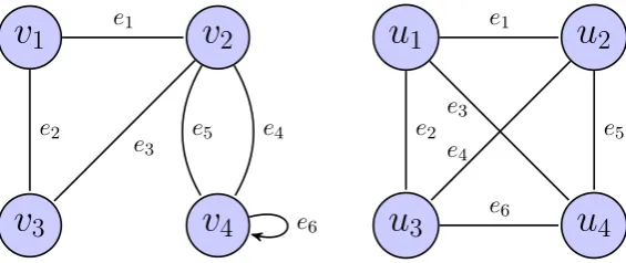
A graph is a representation of a set of objects where some pairs of objects are connected by links. The objects are represented by mathematical abstrac-tions called vertices, and the links are called edges. A graph is commonly depicted as a set of dots for the vertices, joined by lines or curves for the edges. Figure 1.2.1 depicts some example graphs. A simple graph is an undi-rected graph that does not contain loops (edges connected at both ends to the same vertex) and for any pair of verticesuandv it does not contain multiple edges from u to v. A simple graph is commonly defined as an ordered pair
G= (V, E), whereV is the set of vertices andE is the set of edges. An edge is often described as a pair of vertices. Thus if an edgeeconnects the vertices
u and v it can be written as e:= (u, v) (depending on the writer edges may instead be defined as {u, v} or simply uv). Note that in undirected graphs for any edge (u, v) ∈E we will always have that (u, v) = (v, u). A graph is finite if both the set of vertices and the set of edges are finite. In this case
v
1v
2v
3v
4v
5Figure 1.2: two edge disjoint paths that are not vertex disjoint)
vertices have a degree ofk is called ak-regular graph. For v ∈V let N(v;G) be the set of vertices adjacent to v in G.
In graphG1 edge e1 is adjacent to edgee2, as they both have the vertex
v1 in common. The edge e1 is incident to both v1 and v2. Thus vertex v1 is adjacent tov2. The degree of vertexv1 is 2, asv1 is incident to the two edges
e1 and e2. Thus d(v1) = 2. Similarly d(v2) = 4, d(v3) = 2 and d(v4) = 4. Graph G2 is a 3-regular graph, as all vertices ofG2 have a degree of 3.
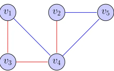
A path in a graph is a finite or infinite sequence of edges which connect a sequence of vertices. A simple path is a path which does not repeat vertices. For example, two possible (simple) paths fromv2tov3inG1 are{e3} {e1, e2}. Two paths are (internally) vertex-disjoint (alternatively, vertex-independent) if they do not have any internal vertex in common. Similarly, two paths are edge-disjoint (or edge-independent) if they do not have any edge in common.
Lemma 1.1. Two internally vertex-disjoint paths are edge-disjoint, but the converse is not necessarily true.
Proof. Let P1 and P2 be internally vertex-disjoint paths in a graph G. As-sume to the contrary that they are not edge disjoint. Then we must have that they both contain the same edge (u, v). However this means that both paths must contain vertices uand v. ForP1 and P2 to be internally vertex-disjoint we must have that u and v are both endpoints of P1 and P2. However as
G is a simple graph (remember that we assume all graphs are simple unless stated otherwise), it then follows that P1 =P2 and thus that P1 and P2 are not edge disjoint.
For the converse note that figure 1.2.1 contains a counterexample where the blue and the red edges are two edge-disjoint paths from v1 to v2, but they are not internally vertex-disjoint as they both contain the same internal vertex v4.
where each two consecutive vertices in the sequence are adjacent to each other in the graph. A circuit can also be defined as a path that starts and ends at the same vertex. A cycle is a circuit where no repetitions of vertices is allowed, other than the necessity of the starting vertex being the same as the ending vertex. A cycle can also be described by its set of edges, instead of a sequence of vertices. In graph G1 an example of a cycle is{v1, v2, v3, v1}, or equivalently {e1, e2, e3}.
Two verticesuandvare connected in a graphG, ifGcontains a path from
u to v. If u and v are not connected in G they are called disconnected. We define a graph G to be connected if all vertex pairs within G are connected.
An edge cut C is a group of edges whose removal disconnects the graph.
Thus a set of edges C ⊆ E is an edge cut if the graph G0 = (V, E \C) is disconnected. We call C ⊆E ak-edge cut if C is an edge cut and|C|=k.
ForX, Y ⊆V denote by Cut(X, Y;G) the set of edges ofGwith one end-point in X\Y and one endpoint inY \X. Letd(X, Y;G) := |Cut(X, Y;G)|. Also, for X ⊆ V define Cut(X;G) := Cut(X, V \X;G) and d(X;G) :=
|Cut(X;G)|. Note that the definition of the function d(X, Y;G) here does not conflict with the degree function d(v;G) defined on vertices, and can be seen as a generalization of it. This is becaused({v};G) =d({v}, V\{v};G) =
|Cut({v}, V \ {v};G)|is the number of edges fromv to the all other vertices in G, which is just the degree of v. Thus we have d({v};G) = d(v;G) and we can use these notations interchangeably.
The edge connectivity of a graph G, for which we will use the notation
λ(G)∈R, is the size of the smallest edge cut in G. We denote by λ(u, v;G) the local edge-connectivity of two vertices u, v in a graph G, which is the size of a smallest edge cut disconnecting u fromv. Menger’s theorem allows us to give an alternative interpretation to local edge-connectivity in terms of edge-independent paths rather than edge cuts: Let x and y be two distinct vertices. The size of the minimum edge cut disconnecting x and y is equal
to the maximum number of pairwise edge-independent paths from x to y.
Note that local k-edge-connectivity is a relation between vertices. It is in fact an equivalence relation as we prove in Lemma 1.2. Let k ∈ Z, a graph
G is called k-edge-connected if the edge connectivity of the graph is at least
k, thus if λ(G)≥k.
Lemma 1.2. Local k-edge-connectivity an equivalence relation.
For transitivity, we need that when λ(u, v)≥k and λ(v, w)≥k, we will also have λ(u, w) ≥ k. Take an arbitrary set of k −1 edges C ( E. As
λ(u, v)≥k,uandv are still connected inG−C (by Menger’s theorem there are at leastk edge disjoint paths fromutov (at least one of these paths still exists after removing the edges in C from the graph G)). The same holds for v and w. Clearly u and w are then also still connected in G−C. As C
was arbitrary we see there exists no k−1 edge cut that disconnects u from
w. Thus λ(u, w)≥k.
A subgraph G0 = (V0, E0) of a graph G = (V, G) is a graph such that
V0 ⊆ V, E0 ⊆E and E0 contains no edges incident to vertices inV \V0. A subgraph G0 is a spanning subgraph of G if Ghas the same vertex set as G. A subgraph G0 of a graphGis said to be an induced subgraph if, for any pair of vertices u, v ∈ G0, the edge (x, y) is contained in G0 if and only if (x, y) is contained in G. Thus an induced subgraph of a graph G has exactly the edges as G over its vertex set, where its vertex set is a subset of G. When an induced subgraph G0 = (V0, E0) of G is k-edge-connected we call G0 a
k-edge-connected component.
Let X ⊆ V be a nonempty set of vertices. We call X(G) ⊆ V a locally k-edge-connected component of G if for every two vertices u, v ∈ X(G) we have that λ(u, v;G) ≥ k. Clearly, if X is a k-edge-connected component it is also a locally k-edge-connected component. Though the reverse does not hold in general.
The definitions for vertex connectivity are similar to those of edge con-nectivity, except that they work with vertex cuts rather than edge cuts. A vertex cut C is a group of vertices whose removal disconnects the graph. Letting E(C) be the sets of edges incident to the vertices C, we have that a set of vertices C⊆V is an vertex cut if the graph G0 = (V \C, E\E(C)) is disconnected. Or equivalently a set of vertices C ⊆V is an vertex cut if the graph induced by V \C is disconnected. We call C ⊆E ak-vertex cut if C
is an vertex cut and |C|=k.
The vertex connectivity of a graphG, for which we will use the notation
κ(G)∈R, is the size of the smallest vertex cut inG. We denote byκ(u, v;G) the local vertex-connectivity of two vertices u, v in a graph G, which is the size of a smallest vertex cut disconnecting u from v. Let k ∈ Z, a graph
G is called k-vertex-connected if the vertex connectivity of the graph is at least k, thus if κ(G) ≥ k. A complete graph is a graph such that every
vertex u ∈ G is adjacent to every other vertex v ∈ G. Graph G2 is an
j = 1, . . . , B, we define ij as the minimum integer such that P ij
l=1b(vl)≥j,
and i0
j as the minimum integer such that
Pi0j
l=1b(vl) ≥ B +j. Notice that
Pij−1
l=1 b(vl) < j holds by definition if ij ≥ 2. Then we can see that ij 6= i0j
since otherwise we would haveb(vij) =
Pij
l=1b(vl)−
Pij−1
l=1 b(vl)>(B+j)−j =
B if ij ≥ 2 and b(vij) ≥ B +j > B otherwise, which contradicts to the
assumption.
LetM ={ej =vijvij0|j = 1, . . . , B}. Then M contains no loop by ij 6=i
0
j.
Moreover GM is a perfect b-matching since |{j|ij = l or i0j = l}| =b(vi), as
required.
In this thesis the problem of finding a minimum cost perfect b-matching is of importance.
Minimum cost perfect
b
-matching
Input: An undirected graph G = (V, E), edge costs we, and a vector
b= (bv :v ∈V) defining the degree requirements.
Output: A a minimum cost set of edgesE0 ⊆Esuch that for all vertices
v, d(v) =b(v)
We call a vertex set X a k-special component in G if X is a locally k -edge-connected component satisfying d(X) ≤ k −1. Note that each vertex with a degree lower than k is trivially a k-special-component.
1.2.2
Metrics
A metric or distance function is a function that defines a distance between elements of a set. If a metric is defined on a set X it must be a function w
of the form w:X×X →R. Such a function w(x, y) is a metric on a setX, if is satisfies the following conditions for all x, y, z ∈X:
• w(x, y)≥0 (non-negativity, or separation axiom),
• w(x, y) = 0 if and only if x = y (identity of indiscernibles, or coinci-dence axiom),
• w(x, y) = w(y, x) (symmetry),
1.3
Approximation Algorithms
For mathematical problems an instance of a problem is a possible input of that problem. For example, for many graph problems an instance of the problem is a specific graph. The set of solutions to a problem is the set of all possible outputs the algorithm may generate. The abstract problem can be seen as the relation that associates an instance of the problem to the correct answer.
Many real-world optimization problem are challenging from a computa-tional standpoint. Large instances of a problem may not be solvable due to the amount of computation that would be needed to find the optimal solution.
An approximation algorithm is an algorithm that runs in polynomial time and finds a solution of provable quality in that its solution is at most a constant factor m larger than that of the optimal solution. Approximation algorithms are commonly used for problems that are N P-hard because, un-less P =N P, it is impossible to find a deterministic algorithm that always finds the optimal solution of the instance in polynomial running time. They are also being used for problems where polynomial running time algorithms that solve the problem optimally are known, but where the running time of these algorithms is too slow for the problems at hand. The approximation ratio of such an algorithm is the bound on how much worse the algorithm’s solution is compared to the optimal solution in the worst case.
An approximation algorithm with an approximation ratio m finds a so-lution to any instance the problem, such that the cost of the soso-lution is at most m·w(OP T), whereOP T is the optimal solution of that instance and
w(OP T) be the cost of this solution.
Such an algorithm is also called an m-approximation algorithm. The smaller the approximation ratio, the better the algorithm is at guaranteeing a low cost solution to the problem. For instance when an algorithm has an approximation ratio of 2, the solution to an instance can be at worst twice as expensive compared to the optimal, but when the approximation ratio is 1.05 the solution can be at most 1.05 times as large.
1.4
Problem Statement
vertices {u, v}, a prescribed value r(u, v) is then given for the needed edge-connectivity (or vertex edge-connectivity). The higher the value r(u, v), the more important it is that vertex u stays connected to vertex v. Rather than spec-ifying a value r(u, v) for each edge (u, v), it may be sufficient to specify a valuer(u) for each vertexu. In this caser(u) is a measure of how important it is to have the vertex u stay connected to the rest of the graph, and u
should stay connected to the rest of the graph if less than r(u) edges are deleted. Some vertices can be considered more important that others and will thus have a higher value for r(u). For instance in a electricity system it is more important that a power plant stays connected than that a single home stays connected to the grid. When every vertex is considered of equal importance regarding connectivity, these connectivity requirements simplify to r(u) =k for some integer k. In this case the problem becomes finding an
k-edge-connected or k-vertex-connected graph. Note that the case of hav-ing connectivity requirements defined on vertices is a special case of the one where we define connectivity requirements for each edge. To see this, note that we can write r(u, v) = max(r(u), r(v)) for all vertices u and v.
When assigning degree constraints the most commonly used constraints either completely fix the degrees of the vertices or bound them from above. These constraints are most commonly used as they tend to arise in various real world problems. As already mentioned, upper bounds are useful when vertices can only handle a certain amount of connections. Fixing the degree specification completely on the other hand can be useful as it can ensure creating a network with a specific structure, such as a ring topology for computer networks.
the following:
• Restriction: When restricting the structure of the input (e.g., requiring distances to be metric), it may be possible to find faster algorithms.
• Parameterization: At times there are fast algorithms when certain pa-rameters of the input are fixed. Many problems have the following form: given an object x and an integer k, does x have some property that depends on k? For instance, when requiring a d-regular k -edge-connected graph, the parameter can be the either the number d or the number k. For some applications the parameter k may be small com-pared to the total input size. For such applications it is useful to have an algorithm whose computation time is exponential only in k.
• Randomized algorithms: Use randomness to get a faster average
run-ning time. Generally randomization algorithms attempt to give a
good performance in the average case over all possible choices of ran-dom input. These algorithms are commonly allowed to fail with some small probability when used on large instances of NP-hard problems to achieve faster running times.
• Heuristic algorithms: The objective of a heuristic is to find a solution in a reasonable time frame that works reasonably well in most cases. For heuristic algorithms there is no proof that the algorithm is both always fast and always produces a good result.
• Approximation algorithms: Instead of searching for an optimal solu-tion, search for a solution that is close to optimal. Unlike heuristics, the solution is required to have a provable solution quality and provable run-time bounds.
In this thesis we will in particular look at the problem of approximating a minimum weightk-edge connectedd-regular graph and the minimum weight
k-vertex connected d-regular graph.
minimum weight
k
-edge connected
d
-regular graph
Input: An undirected complete graph G = (V, E), edge weights w and numbers d, k ∈N with d≥k.
minimum weight
k
-vertex connected
d
-regular graph
Input: An undirected complete graph G = (V, E), edge weights w and numbers d, k ∈N with d≥k.
Output: A minimum weight k-vertex-connected d-regular graph R of
G.
Note that TSP can not be approximated at all when edge weights do not satisfy the triangle inequality [1, 2, 17], and for general T SP it is therefore impossible to find an approximation algorithm unless P =N P.
Lemma 1.4 (proof from pages 30 and 31 of the book Approximation algo-rithms [17]). For any polynomial time computable functionα(n), TSP cannot be approximated within a factor of α(n), unless P = NP.
Proof. Assume, for a contradiction, that there is a factor α(n) polynomial
time approximation algorithm, A, for the general TSP problem. We will
show that A can be used for deciding the Hamiltonian cycle problem (which is NP-hard) in polynomial tine, thus implying P =NP.
The central idea is a reduction from the Hamiltonian cycle problem to the TSP, that transforms a graph G onn vertices to an edge-weighted complete graph G0 onn vertices such that
• if G has an Hamiltonian cycle, then the cost of an optimal TSP tour in G0 isn and
• if G does not have a Hamiltonian cycle, then an optimal TSP tour in
G0 is of cost > α(n)·n
Observe that when run on graph G0, algorithm a must return a solution of cost ≤α(n)·nin the first case, and a solution of cost> α(n)·n in the second case. Thus, it can be used for deciding whether G contains a Hamiltonian cycle.
The reduction is simple. Assign a weight of 1 to edges of G, and a weight of
α(n)·n to nonedges, to obtain G0. Now, ifG has a Hamiltonian cycle, then the corresponding tour in G0 has a cost of n. On the other hand, if G, has no Hamiltonian cycle, any tour in G0 must use an edge of cost α(n)·n, and therefore has cost > α(n)·n.
1.5
Related Work
A lot of research has already been done on network design problems and a lot of approximation algorithms have already been created. Below we review some related work on this subject.
Note that when the connectivity requirements are removed, the problem becomes finding a minimum cost perfect b-matching. This problem can be solved in polynomial time [13, 16]. This is done by extending the graph using a construction that was first observed by Tutte and is described on pages 385 and 386 of the book Matching Theory [13]. This will construct a new graph G0 which contains a perfect matching if and only if the original graph has a perfect b-matching. Afterwards a minimum weight matching is computed over G0. Note that a minimal weight matching can be found in polynomial time [9]. Note that when all vertices are given large degrees some weak connectivity constraints may become trivially satisfied. For instance, when every vertex has a degree of at least |V|/2, any perfect b-matching is automatically connected.
For the case where the degree requirements are removed we get the deter-ministic survivable network design problem (NDP) as mentioned in the moti-vation section. There does not exist a polynomial time algorithm for finding the optimal solution to this problem. However, there do exist approxima-tion algorithms. Jain designed an algorithm for finding a 2-approximaapproxima-tion for the edge-connectivity version of the problem [8]. The algorithm uses the ILP corresponding to the problem. The ILP is relaxed to an LP and is then solved with the ellipsoid algorithm. Then all solutions with value above 0.5 are rounded up to 1 and then these variables are fixed. Now the LP is again solved for the remaining variables and this process is continued until all variables are fixed (the paper proves that there is always at least one edge with a value over 0.5). This process of finding a solution by round-ing up some variables and then solve the residual LP iteratively is called iterative rounding. For the vertex connectivity variant, Kortsarz and Nu-tov gave approximation algorithms for the special case ofk-vertex connected graphs [10]. For arbitrary costs, they designed a k-approximation algorithm for undirected graphs and a (k + 1)-approximation algorithm for directed graphs. For metric costs, they created a (2 + (k−1)/n)-approximation al-gorithm for undirected graphs and a (2 +k/n)-approximation algorithm for directed graphs. When the vertex connectivity requirements can be written as r(u, v) = max(r(u), r(v)) where r(u) is the connectivity requirement for
vertex u, the best known approximation algorithm has an approximation
ratio of 2(k−1), where k= maxu∈V(r(u)) [14].
de-gree constraints are involved.
Recall that TSP asks for a connected graph where each vertex has degree 2. Such a graph is automatically 2-edge-connected as the conditions placed on the graph automatically ensure the graph is a cycle. For the case of TSP where edges satisfy the triangle inequality, Christofides’ approximation algorithm has an approximation ratio of 3/2 [4]. The algorithm is described in Algorithm 1
input : undirected complete graph G= (V, E), edge weights w output: low weight Hamiltonian cycleH (2-edge-connected 2-regular
subgraph) of G
1 Compute a minimum spanning treeT of G.
2 LetVO be the set of vertices with odd degree in T. Compute a
minimum weight perfect matching M in the complete graph over the vertices from VO.
3 Combine the edges ofM and T to form a multigraph H. 4 Form an Eulerian circuitC inH (H is Eulerian because it is
connected, with only even-degree vertices).
5 Obtain a Himiltonian cycleH by skipping repeat visits to vertices of
the circuit C (shortcutting).
Algorithm 1: Christofides algorithm for TSP
Cornelissen et al. [5] designed an approximation algorithm for the problem of finding a 2-edge-connected d-regular subgraph where edge weights satisfy the triangle inequality.
minimum weight 2-edge-connected
d
-regular spanning
sub-graph
Input: An undirected complete graph G = (V, E), edge weights w and an integerk.
Output: A minimum weight spanning subgraph R of G that is
2-edge-connected and d-regular.
Their approximation ratio is 3 when d is odd and 2.5 for even d. The algorithm first computes a minimum cost d-regular graph, which is a special case of a minimum cost b-matching. Then the graph is transformed into a 2-edge-connected graph without changing the degree of any vertex.
in-clude algorithns by Lau et al. [11, 12]. For instance, Lau et al. [11] designed an algorithm for approximating a minimum cost spanning subgraph which satisfies edge-connectivity requirements r(u, v) between vertices and which also satisfies degree upper bounds b+(v) on the vertices. Their result is an (2,2b+(v) + 3)-approximation algorithm. This means that the cost of the graph is at most twice that of the optimal solution and the degree of each vertex v is at most 2b+(v) + 3.
Lau et al. [3] created an algorithm to construct a minimum cost k -edge-connected spanning subgraph under specific degree constraints.
minimum weight
k
-edge-connected
b
-matching
Input: An undirected complete graph G = (V, E), edge weights w and an integer valued function b defined on V and an integerk.
Output: A minimum weight spanning k-edge-connected subgraph R of
G such thatd(v;R) =b(v) for every vertex v.
They proved that anyk-edge-connected graphGcan be transformed into
a graph with maximum degree k + 1 without increasing its cost. As we
already noted there exists a 2-approximation algorithm for finding a mini-mum cost k-edge-connected spanning subgraph [8]. This thus translates into a 2-approximation algorithm for finding a minimum cost k-edge-connected spanning subgraph where each vertex has a maximum degree ofk+ 1. To re-duce the maximum degree down tok the cost of a minimum weight matching needs to be added to the approximation ratio. The cost of such a matching is proven to be at most 1/k times the cost of the minimum weight k -edge-connected subgraph. In total this gives a (2 + 1/k)-approximation algorithm for finding the minimum weight k-edge-connectedk-regular subgraph. Their results can be generalized to the case of general connectivity requirements.
The deterministic survivable network design problem with
degree constraints
Input: An undirected complete graph G = (V, E), edge weights w and an integer valued function b defined on V and a |V| × |V| matrix r
defining the edge connectivity requirements.
Output: A minimum cost set of edges E0 ⊆E such that for all i, j with
i 6=j, there exist at least rij edge disjoint path between vertices i and
j. Furthermore for every vertex v, exactly b(v) edges are incident to v.
Let rmax := maxu,vr(u, v). Any graph G satisfying the general
connec-tivity requirements can be transformed into a graph with maximum degree
algorithm when rmax is even. When rmax is odd this leads to a (4, +1)-approximation algorithm (where the +1 indicates the degree constraints can be off by one and the 4 is the approximation ratio on the cost function). Reducing the maximum degree to rmax in the case of odd rmax gives an 4. 5-approximation ratio instead. For the case of vertex connectivity Lau et al. [3] also find a (2 + k−1
n +
1
k)-approximation algorithm for finding the minimum
k-vertex connected k-regular graph.
One possible alteration to the problem is to allow multigraphs rather than simple graphs. Fukunaga and Nagamochi [6] give an approximation algorithm for finding a minimum cost k-edge-connected multigraph under the constraint that the degree of each vertex v ∈V is equal to a given value
b(v). As additional condition they require thatb(v)≥2 for all verticesv. The problem admits an approximation algorithm with approximation ratio 2.5 if
k is even and an approximation ratio 2.5 + 1.5/k if k is odd. The algorithm first creates a minimum cost perfect b-matching. Then if |V| ≤ 3, this b -matching is the solution. Otherwise a Hamiltonian cycle Gh is computed
using Christodes’ algorithm and this cycle is copied k
2
times. The perfect
b-matching and the k
2
copies of Gh are merged to a single graph. Then
the algorithm uses operations that reduce the number of edges of the perfect
Chapter 2
First Algorithm for
Approximating d-Regular
k-Edge-Connected Subgraphs
In this chapter we will generalize the algorithm of Cornelissen et al. [5]. The original algorithm is a 3-approximation algorithm for the problem of finding a d-regular 2-edge-connected graph. This algorithm start with a minimum weightd-regular graph. Given this graphG, it creates a treeT(G) as follows: The tree has a vertex for every maximum edge-connected subgraph (a 2-edge connected component) of G, and two such vertices are connected in
T(G) if the corresponding 2-edge connected components are connected inG. It is provable that every 2-edge connected component Li(G) of G contains
an edge ei = (ui, vi) for which both ui and vi are not incident to any vertex
outside Li(G).
Then the algorithm of Cornelissen et al. computes a minimum spanning tree and shortcuts it too a Hamiltonian cycle H. This cycle is shortcutted further to create a cycle H0 that trough the vertices {u
1, . . . , uk} where k is
the number of 2-edge connected components. We now assume w.l.o.g. that
H0 traversed these vertices in the order u
1, . . . , uk. Now a d-regular
2-edge-connected graph is constructed by removing the edges (ui, vi) and adding the
edges (ui, vi+1).
approxima-tion for the minimum weight d-regular k-edge-connected spanning subgraph by repeatedly using this algorithm, although the approximation ratio does grow in the size of k.
2.1
Preliminaries
Let us first prove some lemmas on localk-edge-connectivity and on the struc-ture of locally k-edge-connected components.
Lemma 2.1. Let X ⊆ V be a nonempty set of vertices satisfying d(X) ≤
k−1. Assume every vertex in X has at least degree k. Then we must have
|X| ≥k.
Proof. Assume to the contrary that there exists a set of verticesX ⊆V with
d(X)≤k−1 having |X| ≤k−1. Each vertex v ∈X satisfiesd(v)≥k and thus has at leastk neighbours. Also note that each vertexv can have at most
|X|−1 neighbours withinX. Thus, it has at leastd(v)−(|X|−1)≥k+1−|X|
edges to vertices outside of X. Adding over all vertices in X this gives us
d(X)≥(k+ 1− |X|)|X|= (k+ 1)|X| − |X|2 edges to vertices outside ofX. Clearly for |X|= 1 this gives us k+ 1−1 =k and for|X|=k this also gives us (k+ 1)k−k2 =k edges to vertices outside ofX. Noting that this function is a parabola we know that for |X| ∈(1, k) we have d(X)> k. We attained
d(X) ≥ k, which is a contradiction to d(X) ≤ k−1. Thus our assumption of |X|< k was wrong and we must have |X| ≥k.
Corollary 2.2. Assume every vertex in X has at least degreek. Then every k-special-component X satisfies |X| ≥k.
Lemma 2.3. Let G be a (k −1)-edge-connected graph. Every vertex set X (V either contains a k-special-component or satisfies d(X)≥k.
Proof. Assume to the contrary that we can find a setXthat does not contain a k-special-component and satisfiesd(X)≤k−1.
Now let us take a minimal set X with this property. As X is minimal, there is no set of vertices Y ( X that satisfies d(Y) < k and does not contain a k-special-component. Clearly for any set of vertices Y ( X we know Y does not contain ak-special-component as X does not contain such a component (If Y contains a k-special-component, X would also contain that k-special-component as Y (X). Therefore, for each subsetY of X we must have d(Y)≥k.
X does not containk-special-components and thusX cannot be ak -special-component. Thus, X is not locally k-edge-connected. As X is not locally
k-edge-connected, we can find vertices u, v ∈X such that λ(u, v)≤k−1. As λ(u, v) ≤ k−1 there exists an edge cut of size at most k −1 that disconnects u fromv. This cut must split up the graph in two sets U and U
with u∈U, v ∈U, such thatd(U)≤k−1.
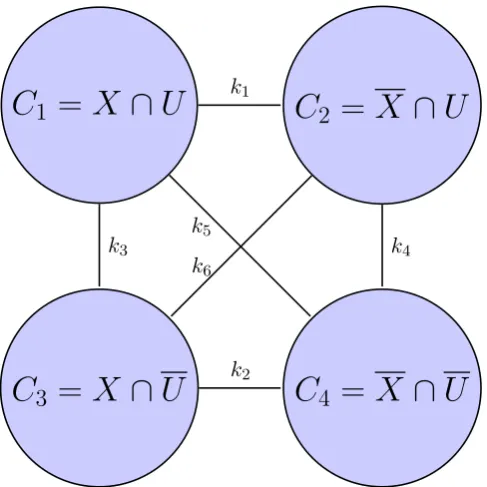
Figure 2.1 illustrates how the graph is split up by these edge cuts. We can now see the graph G as being divided into the following four sections:
• C1 =X∩U,
• C2 =X∩U,
• C3 =X∩U,
• C4 =X∩U.
We can also count the number of edges between these segments as follows:
• k1 is the number of edges between C1 and C2 (k1 =d(C1, C2)),
• k2 is the number of edges between C3 and C4 (k2 =d(C3, C4)),
• k3 is the number of edges between C1 and C3 (k3 =d(C1, C3)),
• k4 is the number of edges between C2 and C4 (k4 =d(C2, C4)),
• k5 is the number of edges between C1 and C4 (k5 =d(C1, C4)),
• k6 is the number of edges between C2 and C3 (k6 =d(C2, C3)).
In the following we specify constraints that the variables{ki, i∈ {1, . . . ,6}}
must satisfy. Then we show that it is impossible to satisfy all these con-straints and thus come to a contradiction. We know that by construction
C1 6= ∅ and C3 6= ∅ (as they contain u and v respectfully). We also know
C2∪C4 6=∅as X is a proper subset of V. However we can have that either
C2 orC4 is empty. Let us first assumeC2, C4 6=∅.
Case 1: C2, C4 6=∅.
First of all we haved(X)< k. This translates intok1+k2+k5+k6 ≤k−1. We also have d(U)≤k−1 and thus k3+k4+k5+k6 ≤k−1.
Note that we haveC1, C3 (Xas by construction we have thatv ∈X∩U and u ∈ X ∩U. We can translate this to constraints k1 +k3+k5 ≥ k and
k2 +k3+k6 ≥k respectively.
C
1=
X
∩
U
C
2=
X
∩
U
C
3=
X
∩
U
C
4=
X
∩
U
k1
k3
k5
k4 k6
k2
Figure 2.1: The graph divided by two edge cuts (one horizontal and the other vertical)
contains at least k − 1 edges. This gives us the following bound on k4:
k4 ≥ k−1−min(k1, k2, k3)−k5 −k6. To see this, note that we want to
find the maximum number of edge independent paths from C2 to C4 that
the graph can possibly have. This total number of paths needs to be at least
k −1. We know that we can have at most one such path for each of the
k4 direct edges and at most min(k1, k2, k3) paths following a detour through
C2, C1, C3, C4. There can then still be paths going trough C2, C3, C4 and
C2, C1, C4, however we can upper bound those by the number of edges k6 and k5 respectfully.
Thus our system of equations becomes:
Find k1, k2, k3, k4, k5, k6 ∈N (2.1.1)
s.t. k1+k2+k5+k6 ≤k−1 (2.1.2)
k3+k4+k5+k6 ≤k−1 (2.1.3)
k3+k1+k5 ≥k (2.1.4)
k3+k2+k6 ≥k (2.1.5)
First note that the constraint 2.1.6 can be rewritten as the following three constraints:
• k4 ≥k−1−k1−k5−k6
• k4 ≥k−1−k2−k5−k6
• k4 ≥k−1−k3−k5−k6
We can rewrite constraint 2.1.3 as k4 ≤ k −1−k3 −k5 −k6. From this constraint and the constraint k4 ≥k−1−k3−k5−k6 we see that we have
k4 =k−1−k3−k5−k6. Filling this in into the equationsk4 ≥k−1−k1−k5−k6 and k4 ≥ k−1−k2 −k5 −k6, we get −k3 ≥ −k1 and −k3 ≥ −k2. Thus
k3 ≤k1 and k3 ≤k2.
We also havek1+k3+k5 ≥k and k2+k3+k6 ≥k which we add giving us the constraint k1+k2+ 2k3+k5+k6 ≥2k. We know k1+k2+k5+k6 ≤
k −1 according to constraint 2.1.2, and we multiply this by two giving us 2k1+ 2k2+ 2k5+ 2k6 ≤2k−2. We know that k3 ≤k1 and k3 ≤k2, thus we also havek1+k2+2k3+2k5+2k6 ≤2k−2. Finally we note that 0≤k5+k6as
k5 andk6 can not be negative, and thus we getk1+k2+2k3+k5+k6 ≤2k−2. Clearly k1+k2+ 2k3+k5+k6 ≥2k andk1+k2+ 2k3+k5+k6 ≤2k−2 can not both be satisfied and thus we have found a contradiction.
Case 2: C2 =∅. Let us assume C2 =∅, we get the following equations
(just a simplification of the equations for the general case): Findk2, k3, k5 ∈N
s.t. k2+k5 ≤k−1
k3+k5 ≤k−1
k3+k5 ≥k
k3+k2 ≥k
Clearly we can not have both k3+k5 ≥k and k3+k5 ≤k−1 leading to an immediate contradiction.
Case 3: C4 =∅. We now get the following equations:
Findk1, k3, k6 ∈N s.t. k1+k6 ≤k−1
k3+k6 ≤k−1
k3+k1 ≥k
k3+k6 ≥k
We find the equations of k3+k6 ≥k and k3+k6 ≤k−1, again leading to a contradiction.
incorrect. As there is no smallest set with this property there exists no set with this property and thus the result follows.
Lemma 2.4. Let X and Y be locally k-edge-connected components in G. If there exists no (k−1)-edge-cut that disconnects X from Y in G, thenX∪Y is a locally k-edge-connected components in G.
Proof. Take an arbitrary x ∈ X and y ∈ Y and take an arbitrary set of (k−1) edgesC. As there exists no (k−1)-edge-cut that disconnectsX from
Y we know that for some wi ∈ X and some wj ∈ Y, wi is still connected
to wj in G−C. As X is a locally k-edge-connected component we know
that in G−C any vertex inX is still connected to every other vertex within
this component (by Menger’s theorem). The same holds for Y. Thus x is
connected to wi and y is connected to wj. Now x is connected to y, as x is
connected to wi, which is connected to wj, which is connected to y. As x, y
and C were arbitrary we have that for every vertex u∈X and every vertex
v ∈ Y we have λ(u, v;G) ≥ k. Thus X ∪Y is a locally k-edge-connected component of G.
The following two lemmas show that we can find a unique list containing allk-special-components of a graph by showing that they are maximal locally
k-edge-connected components and they do not overlap with each other.
Lemma 2.5. Let X be a k-special-component of G, then X is a maximal locally k-edge-connected component of G.
Proof. By definition of k-special-components we know that X is a locally
k-edge-connected component and d(X)< k. As X is nonempty we can find a vertex v ∈ X. Let u 6∈ X. Every path from u to v requires at least one of the edges from Cut(X). A set of i edge disjoint paths from u to v will require at least iof the edges from Cut(X). Asd(X)< kthere exist at most
k−1 such edges and thus there exist at mostk−1 edge disjoint paths from
u to v. Thus λ(u, v) ≤ k −1. As v was arbitrary we see that no vertex
v 6∈X is locallyk-edge-connected touand thus we can not addv toX while still keeping X a locallyk-edge-connected component. Thus X is a maximal
k-edge-connected component of G.
Corollary 2.6. If U and X arek-special-components of G, then either U =
X or U ∩X =∅.
Proof. Assume thatU∩X 6=∅and thus that there exists a vertexu∈U∩X.
discon-ui touj. From Lemma 2.13 we know that if a k−1 edge cut disconnectsuk
from vk then it is impossible for that cut to also disconnects ul from vl for
any l 6=k. Thus there can be at most one pair (uk, vk) that is disconnected
by the k −1 edge cut. However this means that either path P1 or path P2 connects ui touj. This follows from the fact that we have edges going from
each ui to each vi+1 and for only a single k we can not find a path from vk
to uk to connect these (ui, vi+1) edges into a path (only one path P1 or P2 requires a path from vk to uk, thus the other path is a valid path contained
inR−C). We have now proven thatui is connected to uj inG−C which is
a contradiction. Thus we can not find a k−1 edge cut disconnecting some verticesui anduj from each other. Thus for alli, j ∈ {1, . . . , m}we have that
ui and uj are locallyk-edge-connected with each other in the new graph.
Lemma 2.18. InR =G+S−Q as created by Algorithm 2 we have that Li
and Lj are locally k-edge-connected for all i, j ∈ {1, . . . , m}.
Proof. To prove this lemma we want to show that every vertex v ∈Li is
lo-cally k-edge-connected to every vertex u∈Lj for arbitrary i and j. Lemma
2.17 already gives us this result if we choose v =ui and u=uj. We first
ex-tend this by adding the option of choosing verticesvi. We know that for alli,
ui−1andvi are locallyk-edge-connected. We also already knowui−1 is locally
k-edge-connected to any uj. Thus using the fact that k-edge-connectivity is
transitive, we find that all vertices vi are locally k-edge-connected to all ui
and all other vj.
Now take some vertex v ∈ Li with v 6=ui and v 6=vi. We need to prove
that it is locally k-edge-connected to ui. Let us assume to the contrary that
v is not locally k-edge-connected toui and thus that we can find ak−1 edge
cut C disconnecting v fromui. AsG−Q is (k−1)-edge-connected we know
allk−1 of the edges inC are not contained inS. Thus we can also take this cut in the original graph G. We know v and ui are locallyk-edge-connected
in G. Thus there is still a path from v to ui in G−C. Necessarily it uses
one or more edges (uj, vj) ∈ Q, as they are the only edges contained in R
that are not contained in G−Q (otherwise the path would exist in R−C
and thus C would not be an edge cut disconnectingv fromui). Let us write
the path from v to ui as P1(uj, vj)P2. As we already showed each uj and
vj are locally k-edge-connected in G−Q+S, we know that uj and vj are
still connected in G−Q+S −C. Thus we can find a path P3 contained in G−Q+S −C, that connects ui and vi. Thus we have a path P1P3P2 going fromv toui. Note thatP3 contains no edges (ui, vi)∈Qand thus this
new path P1P3P2 has a lower number of edges contained in Q compared to the old path P1(uj, vj)P2. We can repeat this procedure for any other edge
ui only uses edges withinG+S−Q. Thus contradicting our assumption that
a k −1 edge cut C disconnecting v from ui exists. Thus we have that that
any vertex v ∈Li is locally k-edge-connected toui. We have by transitivity
of k-edge-connectivity that every vertex v ∈ Li is locally k-edge-connected
to every vertex u∈Lj for arbitraryi and j.
Theorem 2.19. The graph R = G+S −Q as created by Algorithm 2 is k-edge-connected.
Proof. Our previous Lemma already gave us the result that Li and Lj are
locally k-edge-connected for all i, j ∈ {1, . . . , m}.
Thus we are only left to look at the vertices not contained in any com-ponents Li. Let v be a vertex not contained in one of the components and
assume that we have a k−1 edge cut C disconnecting it from a part of the graph. Take the largest set X such that v ∈X and every vertex in X is con-nected tov inG−C. We now know d(X;R−C) = 0 as otherwise we would have taken a larger set X. As |C| ≤k−1 we have d(X;R)≤ k−1. From Lemma 2.3 we know that d(X) ≥k for any set X that does not contain an
k-special-component (as we already know G isk−1 edge connected). Thus
X has to contain some k-special-component Li. Thus, after the edge cut, v
is still connected to a vertex u within one of the components Li.
AsC was arbitrary we find that there exists no k−1 edge cut such that
v is disconnected from all vertices of S
iLi inG. As to create R fromG the
only edges we removed were edges connecting two vertices within S
iLi we
know that this property also holds for the graph R =G+S−Q.
We have already proven that S
iLi is a locally k-edge-connected
compo-nent. A single vertex is a trivial locally k-edge-connected component. Thus we can use Lemma 2.4 to find thatvis locallyk-edge-connected to all vertices inS
iLi. Finally as localk-edge-connectivity is transitive andvwas arbitrary
we find that the entire vertex setX is a locallyk-edge-connected component in R. From this it immaterially follows that R is a k-edge-connected graph.
Lemma 2.20. Assume that the graph R is computed as in Algorithm 2 and let G be the input graph of Algorithm 2. Let M ST be the minimum weight spanning tree. We have w(R)≤w(G) + 2w(M ST).
correctness of this algorithm is now trivial as there exist algorithms for cre-ating a minimum cost perfect b-matching in polynomial time, and we have already proven that 2 works correctly in increasing the edge connectivity of a graph without changing the degree of any vertex.
input : undirected complete graph G= (V, E), edge weights w,
k ∈N, and a vector b= (bv :v ∈V) defining the degree
requirements with the restriction thatbv ≥2
k
2
for allv ∈V output: k-edge-connected spanning subgraph R of G, satisfying
d(v;R) = bv for all vertices v ∈V
1 Compute a minimum cost perfect b-matching G0 of G 2 for p= 1. . . k do
3 Apply algorithm 2 to create a p-edge-connected graphG00 of G0
satisfying d(v;R) = bv for all vertices v ∈V 4 G0 ←G00
5 end
Algorithm 4: Creating a k-edge-connected spanning subgraph, satis-fying degree constraints, with bounded weight
Theorem 2.23. Let R be the k-edge-connected spanning subgraph, satis-fying degree constraints, as was created with Algorithm 4 and let GOP T
k,b be
the minimum weight k-edge-connected b-matching. We have w(R) ≤ (2k+ 1)w(GOP T
k,b ).
Proof. LetG−,b be a minimum weight b-matching and let M ST be the
min-imum weight spanning tree. Note that the algorithm will have a total of k
iterations, and note that by Lemma 2.20 each iterations adds a weight of at most 2w(M ST) to the graph from the previous iteration. Thus we get
w(R)≤w(G−,b) + 2kw(M ST). We have that w(M ST)≤w(GOP Tk,b ) as GOP Tk,b
is a connected graph and M ST is a minimum weight connected graph. Also
GOP T
k,b is a b-matching, while G−,b is a minimum weight b-matching and thus
Chapter 3
Second Algorithm for
Approximating d-Regular
k-Edge-Connected Subgraph
Assume we have a k-edge-connected graph Gk,k = (Ek,k, Vk,k) where each
vertex has maximum degree k and a d-regular graph G−,d = (E−,d, V−,d).
We wish to create a k-edge-connected d-regular graph Gk,d. We do so by
starting with G−,d, which is d-regular, and adding edges of Gk,k without
changing the degree of any vertex (by removing other edges) until the new graph Gk,d is alsok-edge-connected. (It is impossible for Gk,d not to become
k-edge-connected in this process, as after adding all edges of Gk,k we would
have that Gk,k is a subgraph of Gk,d thus immaterially implying that Gk,d is
k-edge-connected.) First note that if d = k then Gk,k is d-regular as each
vertex has maximum degree k and for k-edge-connectedness each vertex has to have at least degree k. Thus we can take Gk,d = Gk,k. Thus we can
assume d > k which implies that for each vertex v ∈ G−,d there is at least
one edge e = (v, u) ∈ G−,d with e 6∈ Gk,k. Also note that as long as Gk,k
is not a subgraph of G−,d (at which point we are surely done) there always
exists some edge e∈Gk,k with e6∈G−,d.
Algorithm 5 is our approximation algorithm for creating ak-edge-connected
d-regular graph for the case where d≥2k−1. Each loop we add an edge of
Gk,k to Gk,d. Then to keep Gk,d a d-regular graph we remove two edges in
Gk,d incident to the newly added edge and add the edge connecting the two
endpoints u2 and v2 of these newly added edges. To keep the graph simple we require that none of the two newly added edges is already contained in
Gk,d. We shall later show that as long as Gk,d is not k-edge-connected and
input : undirected complete graph G, edge weights w,d, k ∈N
satisfying d≥2k−1, k-edge-connected subgraph Gk,k of G
where each vertex has maximum degree k, a d-regular subgraph G−,d of G
output: k-edge-connectedd-factor Gk,d of G 1 Gk,d←G−,d
2 while Gk,d is not k-edge-connected do
3 Take an edge (u1, v1)∈Gk,k with (u1, v1)∈/ Gk,d and add it toGk,d 4 Remove some edges (v1, u2),(u1, v2) from Gk,d that are not
contained in Gk,k.
5 Add an edge (u2, v2)6∈Gk,d to Gk,d and go to step 2 6 end
Algorithm 5: Second algorithm for creating a k-edge-connected d -regular graph with bounded weight
Lemma 3.1. The graph Gk,d created by algorithm 5 is a d-regular graph.
Proof. First note that at the start of the algorithm Gk,d is d-regular as G−,d
is d-regular. Thus we only need to prove that after every iteration of the loop the graph remains d-regular. In this algorithm we add edges (u1, v1) and (u2, v2) and we remove edges (u1, v2) and (u2, v1). Thus for for all four of these vertices we remove one adjacent edge and add an adjacent edge, leaving their degree the same. The degree of all other vertices does not change at all during the loop. At the end of the loop every vertex still has the same degree as at the beginning of the loop and thus Gk,d is still d-regular.
Lemma 3.2. The graph Gk,d created by by algorithm 5 is a simple graph.
Proof. Initially Gk,d is a simple graph as G−,d is a simple graph. Any edge
we add during the algorithm is an edge that at that time is not already contained within Gk,d. Thus at any point in the algorithm, Gk,d remains a
simple graph.
Lemma 3.3. The graph Gk,d created by by algorithm 5 is k-edge-connected.
Proof. If the algorithm terminates, this is trivial.
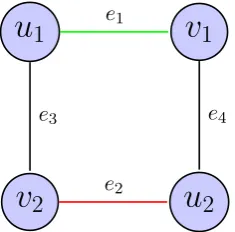
Lemma 3.4. Assume d≥2k−1, ifGk,d is notk-edge-connected we can find
two edges e1 = (u1, v1), e2 = (u2, v2) satisfying the following conditions:
u
1v
1v
2u
2e1
e3 e4
e2
Figure 3.1: Picture for the proof of Lemma 3.4. The cycle we wish to con-struct in Lemma 3.4.
2. e1 ∈Gk,k
3. There exist edges e3 and e4, adjacent to both e1 and e2, satisfying
e3, e4 ∈ Gk,d and e3, e4 ∈/ Gk,k (w.l.o.g. we can assume e3 = (u1, v2)
and e4 = (v1, u2)
Proof. If Gk,d is not k-edge-connected than we know there exists a vertex
set X with d(X) ≤ k −1 in Gk,d. As Gk,k is k-edge-connected we know
d(X) ≥ k in Gk,k. Thus there exists at least one edge e1 = (u1, v1) ∈ Gk,k
with e1 6∈Gk,d going from X to X.
AsGk,k has maximum degreekwe know thatu1 andv1 have at mostk−1 incident edges that are contained in both Gk,d andGk,k. AsGk,d is d-regular
we thus have that u1 and v1 have at least d−k+ 1 other edges in Gk,d, all
of which are not contained in Gk,k. Thus we have d−k+ 1 choices for u2 and v2 such that e3, e4 ∈Gk,d and e3, e4 ∈/ Gk,k. We are done if it is possible
to choose u2 and v2 such that the edge e2 = (u2, v2) is not contained in Gk,d.
As then we have that e1, e2 ∈/ Gk,d, e1 ∈ Gk,k and e1 and e2 are incident to two edges e3 and e4 satisfying e3, e4 ∈Gk,d and e3, e4 ∈/ Gk,k thus satisfying
all conditions of the lemma.
Our result follows after we have proven that we can find such an edge
e2 = (u2, v2).
Thus assume to the contrary that all choices foru2 and v2 lead to either the existence of an edge (u2, v2) in Gk,d or to u2 =v2. We can find a contra-diction by proving that d(X)≥k. Refer to figure 3 as an illustration of the following construction.
Let u∗
i with i ∈ {1, . . . ,1 +d−k} be the possible choices for u2 and vi∗
with i ∈ {1, . . . ,1 +d−k} be the possible choices for v2. For any i and j
where u∗
i = v∗j we have the following path from u1 to v1: (u1, u∗i = vj∗, v1). Now remove the vertices for which u∗
u
1v
1u
01u
02u
0k−1u
∗1=
v
1∗u
∗2=
v
2∗u
∗p=
v
p∗u
∗p+1u
∗p+2u
∗p+3u
∗d−k+1v
10v
20v
k0−1v
p∗+1v
p∗+2v
p∗+3v
d∗−k+1 e1Figure 3.2: Picture for the proof of Lemma 3.4. Blue edges are a part ofGd,d
and possibly also of Gk,d, the green edge only exists in Gd,d and we prove
that at least one of the red edges does not exist in Gk,d. (There are possibly
more than d−k+ 1 vertices connected to ui orvi via black edges, although
algorithm we have a cycle consisting of four edges (e1, e2, e3, e4), where e1 ∈
Gk,k and e3 are added, while e2, e4 ∈ G−,d are removed from Gk,d. By the
triangle inequality we know that w(e3) ≤ w(e4) +w(e1) +w(e2). Thus we know the weight we added to Gk,d equals w(e1) +w(e3)−w(e2)−w(e4) ≤
2w(e1). As we alterGk,dat most once for every edgee1 ∈Gk,kand at the start
of the algorithm we haveGk,d =G−,d, we havew(Gk,d)≤w(G−,d)+2w(Gk,k).
Let GOP T
k,d be the minimal weight k-edge-connected d-regular graph. For
G−,d we can find the minimum weight d-regular graph. Clearly we have
w(G−,d)≤w(Gk,dOP T) asGOP Tk,d is also ad-regular graph andG−,dhas minimum
weight amongst the d-regular graphs. For Gk,k we can find a low weight k
-regular k-edge-connected graph that is at most 2 + 1
k times as expensive as
the minimum weightk-edge connected graph. Thus asGOP T
k,d is also ak-edge
connected graph we havew(Gk,k)≤(2 +k1)w(GOP Tk,d ). Putting it all together
we find that w(Gk,d)≤w(G−,d) + 2w(Gk,k)≤(5 + 2k)w(G)
3.1
Vertex Connectivity Case
Algorithm 5 does in fact also work when we replace edge connectivity with vertex connectivity resulting in Algorithm 6.
input : undirected complete graph G, edge weights w,d, k ∈N
satisfying d≥2k−1, k-vertex-connected subgraph Gk,k of G
where each vertex has maximum degree k, a d-regular subgraph G−,d of G
output: k-vertex-connectedd-factor Gk,d of G 1 Gk,d←G−,d
2 while Gk,d is not k-vertex-connected do
3 Take an edge (u1, v1)∈Gk,k with (u1, v1)∈/ Gk,d and add it toGk,d 4 Remove some edges (v1, u2),(u1, v2) from Gk,d that are not
contained in Gk,k.
5 Add an edge (u2, v2)6∈Gk,d to Gk,d and go to step 2 6 end
Algorithm 6: Algorithm for creating a k-vertex-connected d-regular graph with bounded weight
This time we assume we have ak-vertex-connected graphGk,k = (Ek,k, Vk,k)
where each vertex has maximum degree k, rather than a k-edge-connected graph. We still have our d-regular graph G−,d = (E−,d, V−,d) and we now
exactly the same as before except now checking if Gk,d isk-vertex-connected
rather then checking for edge connectivity:
The only Lemmas that used the fact that Gk,k is k-edge-connected are
Lemma 3.4 and Lemma 3.6.
For Lemma 3.4 we note that we foundk vertex disjoint paths rather than just k edge disjoint paths from u1 tov1. Additionally we now start out with a ui and a vi that are disconnected by a k−1 vertex cut rather than by a
k−1 edge cut. However outside of these details the proof remains the same. For completeness we have added the proof of Lemma 3.4 for the k-vertex connected case below.
Lemma 3.7. Assume d ≥ 2k−1, if Gk,d is not k-vertex-connected we can
find two edges e1 = (u1, v1), e2 = (u2, v2)s satisfying the following conditions:
1. e1, e2 ∈/Gk,d
2. e1 ∈Gk,k
3. e1 ande2 are incident to two edgese3 ande4 satisfyinge3, e4 ∈Gk,dand
e3, e4 ∈/Gk,k (w.l.o.g. we can assume e3 = (u1, v2) and e3 = (v1, u2)
Proof. As Gk,d is not k-vertex-connected there must be some edges e1 = (u1, v1) contained inGk,k that are not contained in Gk,d.
Recall that Gk,d is k-vertex-connected if |V| > k (which should always
be true due to the minimum degree of each vertex) and |N(X)| ≥ k for all nonempty X ⊆V with |X| ≤ |V| −k. AsGk,d is notk-vertex-connected we
can thus find a set X ⊆V with |X| ≤ |V| −k and |N(X)| ≤k−1. AsGk,k
is k-vertex-connected we also know |N(X)| ≥ k in Gk,k. Thus there exists
some edge going fromX toXcontained inGk,k that is not contained inGk,d.
Choose one such edge to be e1 = (u1, v1) (Thus we ensured e1 ∈ Gk,k and
e1 ∈/Gk,d.) We can assume w.l.o.g. that u1 ∈X and v1 ∈/ X.
As Gk,k has maximum degree k we know that u1 and v1 have at most
k −1 incident edges that are contained in both Gk,d and Gk,k. As Gk,d is
d-regular we thus have that u1 and v1 have at least d−k+ 1 other edges in
Gk,d, all of which are not contained in Gk,k. Thus we haved−k+ 1 choices
for u2 and v2 such that e3, e4 ∈ Gk,d and e3, e4 ∈/ Gk,k. We are done if it is
possible to choose u2 andv2 such that the edge e2 = (u2, v2) is not contained in Gk,d and u2 6= v2 (this latter condition is required as Gk,d must remain a
simple graph). As then we have that e1, e2 ∈/ Gk,d, e1 ∈ Gk,k and e1 and e2 are incident to two edges e3 and e4 satisfying e3, e4 ∈Gk,d and e3, e4 ∈/ Gk,k
Chapter 4
Summary and future work
4.1
Summary
In this thesis we have described various problems involving the creation of low cost networks that satisfy certain connectivity requirements, and sum-marized some of the work that has been done in this area. We then described two approximation algorithms for creating a low weight k-edge-connectedd -regular subgraph under the assumption that edge weights satisfy the triangle inequality and proved their correctness.
The first of these algorithms is Algorithm 3, which gives a (2k−1) ap-proximation ratio under the condition that d ≥ 2k
2
. This algorithm can also be generalized to work with arbitrary degree requirementsbv, where each
vertex v is to have a degree of bv. This results in Algorithm 4, which has an
approximation ratio of (2k+ 1) and requires thatbv ≥2
k
2
for all vertices
v.
The second algorithm is Algorithm 5, which gives a (5+2k) approximation ratio, but requires the restriction thatd≥2k−1. The same type of algorithm can also be used for creating a low weight k-vertex-connected d-regular sub-graph. This results in Algorithm 6 which is an (5 +2(kn−1)+2k)-approximation algorithm for the minimum weight k-vertex-connectedd-regular graph prob-lem. This algorithm also requires the restriction that d≥2k−1.
4.2
Future work
Algorithm 3 and Algorithm 4 require that every vertex needs to have a degree of at least 2k
2
could for instance be useful in real world problems where one wants to create a connected graph and some vertices are to have a degree of one. For this case one can use algorithm Algorithm 4, but there will be some connected components that do not contain a 2-edge-connected components, which the current algorithm requires for its proof of correctness. One can still apply the algorithm on the components that do have 2-edge-connected components, but after the algorithm ends there will still be some componentsT1, ..., Tc (which
will be trees) that are not connected to the rest of the graphR. If the original degree specification bv is feasible, it is possible to connect these trees to the
rest of the graph. One option to do so would be to remove an edge contained in a cycle of R and an edge contained in some tree Ti and to subsequently
connect the incident vertices of the tree, with those of the cycle. Doing this for every treeTi would create a connected graph with the degree specification
bv. It is still uncertain if such an approach can be proven to have a solution
Bibliography
[1] Markus Bl¨aser, A new approximation algorithm for the asymmetric tsp with triangle inequality, ACM Transactions on Algorithms 4 (2008), no. 4.
[2] Markus Bl¨aser, Bodo Manthey, and Jiri Sgall, An improved approxi-mation algorithm for the asymmetric TSP with strengthened triangle inequality, J. Discrete Algorithms 4 (2006), no. 4, 623–632.
[3] Yuk Hei Chan, Wai Shing Fung, Lap Chi Lau, and Chun Kong Yung,
Degree bounded network design with metric costs, SIAM J. Comput.40
(2011), no. 4, 953–980.
[4] N. Christofides,Worst-case analysis of a new heuristic for the traveling salesman problem, (1976).
[5] Kamiel Cornelissen, Ruben Hoeksma, Bodo Manthey, N. S.
Narayanaswamy, and C. S. Rahul,Approximability of connected factors, WAOA, 2013, pp. 120–131.
[6] Takuro Fukunaga and Hiroshi Nagamochi, Network design with
edge-connectivity and degree constraints, Theory Comput. Syst. 45 (2009), no. 3, 512–532.
[7] Martin Gr¨otschel and Clyde L. Monma, Integer polyhedra arising from certain network design problems with connectivity constraints, SIAM J. Discret. Math. 3 (1990), no. 4, 502–523.
[8] Kamal Jain, A factor 2 approximation algorithm for the generalized steiner network problem, Combinatorica 21 (2001), no. 1, 39–60.
[10] Guy Kortsarz and Zeev Nutov, Approximating node connectivity prob-lems via set covers, Algorithmica37 (2003), no. 2, 75–92.
[11] Lap Chi Lau, Joseph Naor, Mohammad R. Salavatipour, and Mohit Singh,Survivable network design with degree or order constraints, SIAM J. Comput. 39 (2009), no. 3, 1062–1087.
[12] Lap Chi Lau and Mohit Singh, Additive approximation for bounded de-gree survivable network design, SIAM J. Comput.42(2013), no. 6, 2217– 2242.
[13] Laszlo Lovasz and Michael D. Plummer, Matching Theory, American
Mathematical Society, August 1986.
[14] Zeev Nutov, Approximating multiroot 3-outconnected subgraphs, Net-works 36 (2000), no. 3, 172–179.
[15] M. Resende and P. (eds.) Pardalos, Handbook of Optimization in
Telecommunications, 1 ed., Springer, March 2006.
[16] Alexander Schrijver, Combinatorial Optimization : Polyhedra and Effi-ciency, Algorithms and Combinatorics, Springer, July 2004.
[17] Vijay V. Vazirani, Approximation algorithms, Springer-Verlag New
York, Inc., New York, NY, USA, 2001.
[18] Leonardo Zambito, The traveling salesman problem: A
comprehen-sive survey, (2006), http://www.cse.yorku.ca/~aaw/Zambito/TSP_