Machine Learning Verdict of EEG Signals in Brain Computer Interface

(1)

Machine Learning Verdict of EEG Signals in Brain Computer

Interface

M. Jeyanthi, Dr. C. Velayutham

Department of Computer Science, Aditanar College of Arts and Science, Tiruchendur, affiliated to Manonmaniam Sundaranar University, Tirunelveli, Tamil Nadu, India

ABSTRACT

In Science and Technology Development BCI plays a vital role in the field of Research. Classification is a data mining technique used to predict group membership for data instances. Analyses of BCI data are challenging because feature extraction and classification of these data are more difficult as compared with those applied to raw data. In this paper, We extracted features using statistical Haralick features from the raw EEG data. Then the features are Normalized. Binning is used to improve the accuracy of the predictive models by reducing noise and eliminate some irrelevant attributes and then the classification is performed using different classification techniques such as Naïve Bayes, k-nearest neighbor classifier, SVM classifier using BCI dataset. Finally we propose the SVM classification algorithm for the BCI data set.

Keywords: BCI, Classification, KNN, SVM, Data mining.

I.

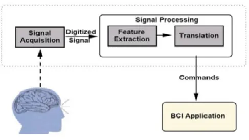
INTRODUCTION

Brain-computer interface (BCI) is a fast growing emergent technology, in which researchers aim to build a direct channel between the human brain and the computer. BCI is a technology which allows a human to control a computer, peripheral or other electronic device with thought. It does so by using electrodes to detect electric signals in the brain which are sent to the computer. The computer then translates these electric signals into data which is used to control a computer or a device linked to a computer.

Classification is used to classify each item in a set of data into one of predefined set of classes or groups. The data analysis task classification is where a model or classifier is constructed to predict categorical labels (the class label attributes). Classification is a data

mining function that assigns items in a collection to target categories or classes. The goal of classification is to accurately predict the target class for each case in the data.

Figure 1 : Basic Block Diagram of a BCI system incorporating signal detection, processing and

(2)

Early works in this area, i.e., algorithms to reconstruct movements from motor cortex neurons which control movement, were developed in the 1970’s. The first intra-cortical BCI was built by implanting electrodes into monkeys. After conducting initial studies in rats during 1990’s researchers developed brain computer interfaces that decoded brain activity in monkeys and used the devices to reproduce the movements in monkeys and then used the devices to reproduce monkey movements in robotic arms.

The organisation of the paper as follows : Section II shortly describes the Literature Review, Section III describes the BCI data set, Section IV describes the Feature Extraction, Section V describes the Normalization, Section VI describes the Feature Selection, Section VII presents the Discretization methods, Section VIII briefly discuss about the Classification Algorithms, Section IX presents the Measures of classification Performance, Section X presents the Results and Discussions and Section XI concludes the paper.

II.

LITERATURE REVIEW

Today , there are more literature mainly focused on Zhao et al., in [1] proposed an Incremental Common Spatial Pattern (ICSP) algorithm to solve the poor adaptability of CSP. The new method interpreted CSP feature extraction using the framework of Rayleigh coefficient maximization. An iterative equation of spatial filter was deduced with the present covariance matrices of the two classes and the old spatial filter. The distinct advantage of ICSP was lower computational cost compared to re-training the whole data, so it was more suitable for development of on-line BCI system.

Oskoei et al., (2009)[2] mainly focused on designing an adaptive classifier , since a classifier is the core of

pattern recognition – based BCI. A variety of adaptive schemes based on some common classifiers such as linear discriminant analysis (LDA).

Vidaurre et al., (2011; 2007; 2008)[3][4][5], quadratic discriminant analys)is (QDA)[6], support vector machine (SVM) (Oskoei et al., 2009; 2007) and so on have been proposed in recent years. The principles of the above algorithms were aimed at adjusting the separating hyper plane along with the changing distribution of features. Vidaurre et al., (2007) had done a comprehensive work in this area. They proposed two continuously adaptive classifiers based on QDA and LDA, while analysing the adaptive autoregressive parameters and the logarithmic band power in feature type.

Grychtol et al., (2010)[6] investigated the effects of feedback and motivation on the performance of BCI, and it represented many new interesting results in actual online BCI.

Yoon et al., (2009)[7] proposed two new algorithms to handle missing or erroneous labeling in BCI data: the auxiliary label and the optimal proposal functions had been applied successfully to BCI data.

Artificial neural network Huang et al., (1996;1999; 2008)[8][9][10] as a powerful tool in pattern recognition was also applied in the BCI.

Hazrati et al., (2010)[11] had designed an adaptive probabilistic neural networkworking in a time-varying environment for classification of EEG signals, which reached a higher accuracy level of classification over different sessions and subjects.

(3)

Bayesian Model relies on a good amount of samples. That may lead to performance degradation when facing the problem that the initial EEG data which is used to constitute the initial training set is limited. As a matter of fact, because of the individual differences and the influence of EEG non- stationary (i.e. even for the same subject, it is hard to employ the same classifier without retraining to classify the data collected on two different time), before starting to use an online BCI, there should be a training procedure for the subject that the data acquired are used for off-line training classifier. Unfortunately, the size of the initial data is usually small for time efficiency and subject fatigue, so how to tackle with the adaptive classification in the circumstance of small-sample also ought to be considered.

MihaelaMaracine et al., (2017)[14]The paper is also focused on the study of classification algorithms that can be optimal candidates for signals classification obtained in order to identify right and left hand movement. Two types of neural networks based classifiers are used and tested in order to compare the results - Multi-Layer Perceptron (MLP) and Radial Basis Function (RBF), two types of linear classifiers – Linear Discriminant Analysis and Support Vector Machine and K Nearest Neighbor (KNN).

F Lotte et al., (2018)[15] designed classification algorithms for EEG-based BCIs can be divided into four main categories: adaptive classifiers, matrix and tensor classifiers, transfer learning and deep learning, plus a few other miscellaneous classifiers. Among these, adaptive classifiers were demonstrated to be generally superior to static ones, even with unsupervised adaptation. Transfer learning can also prove useful although the benefits of transfer learning remain unpredictable. Riemannian geometry-based methods have reached state-of-the-art performances on multiple BCI problems and deserve to be explored more thoroughly, along with tensor based methods. Shrinkage linear discriminant

analysis and random forests also appear particularly useful for small training samples settings.

Yongkoo Park et al., (2018)[16] This paper is also focused on the study of novel motor imagery classification method in electroencephalography (EEG)-based Brain-Computer Interfaces (BCIs) using locally generated CSP features centered at each channel. By favoring the channels with the local CSP features exhibiting significant eigen value disparity in the classification stage ,improved performance in classification accuracy can be achieved in comparison with the conventional globally optimized CSP feature, especially for small-sample setting environments. Simulation results confirm the significant performance improvement of the proposed method for BCI competition III dataset IVa using 18 channels in the motor area.

Keum-Shik Hong et al.,(2018)[17]This paper focused recent work on functional near infrared spectroscopy (fNIRS) and hybrid fNIRS-EEG studies for brain-computer interfaces (BCI). The focus was on finding the brain activity patterns, channel selection criteria, feature extraction schemes, and classification algorithms that are most suitable for locked-in patients.

Hardik et al., (2018)[18] This paper focused on common spatial pattern algorithm for multiclass EEG classification with a pre-processing step which can improve the generalization of CSP covariance matrices by removing the trials which are noisy/affected with arte fact. SRIT2NFIS is used as a classifier to handle the non stationary present in the signal. The results were presented on publically available data set BCI competition IV data 2a. Results are compared with the currently state of the art algorithms for multiclass classification.

(4)

Experimental paradigm

The data sets of EEG data were recorded from several healthy subjects. The cue-based BCI paradigm consisted of two/three motor imagery tasks, namely the imagination of movement of the left hand (LH), right hand (RH) and both feet (F). Several sessions on different days were recorded for some subjects, the data of each session was stored in one data file respectively. In this work we consider only the two class datasets.

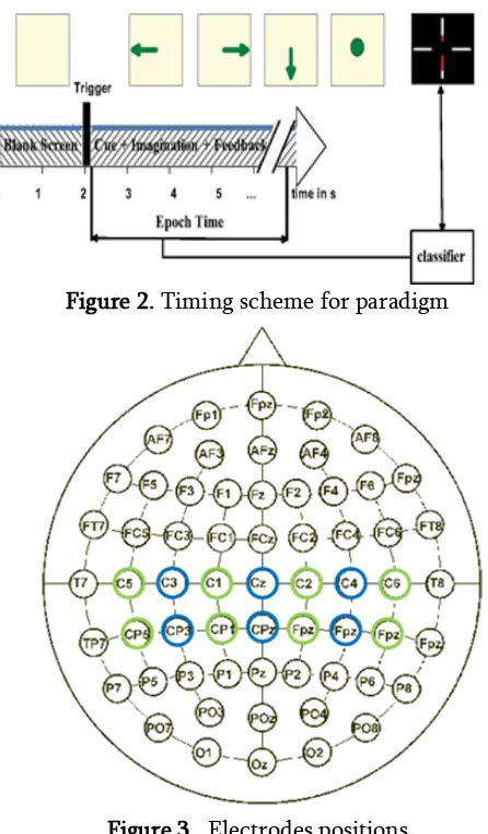
The subjects were sitting in a comfortable armchair in front of a computer screen. At the beginning of a trial, the screen is blank. After two seconds (t=2s), a cue in the form of an arrow pointing either to the left, right or down (corresponding to three classes of LH, RH and F) appeared and stayed on the screen for a specific duration (3-10 sec). This prompted the subjects to perform the desired motor imagery task. The subjects were requested to carry out the motor imagery task until the cue disappeared from the screen and try to avoid the eye blinking or eye movements during the imagination. A 2 seconds break followed when the cue is disappeared. This procedure is repeated 30-100 times for each run with the random cue sequence. The paradigm is illustrated in Figure 2. For each subject, the first run is called initialization procedure which only presents the cues without any feedback. Based on the online BCI classifier trained on the EEG data recorded from the initialization run, the system is able to present the system feedback online by several red bars representing the classification output for left hand, right hand and feet commands. Meanwhile, the EEG data with class labels are recorded. The experiments conducted in different days for the same subject are called different sessions.

Figure 2. Timing scheme for paradigm

Figure 3. Electrodes positions

Data recording

In this data sets, the two devices of g.tec (g.USBamp) and Neuroscan (SynAmps RT) were used for recording the EEG signals. The EEG signals were band-pass filtered between 2Hz and 30Hz with sample rate of 256Hz and a notch filter at 50Hz was enabled for g.tec whereas the band-pass filter between 0.1Hz and 100Hz with sample rate of 250Hz was applied for Neuroscan device. The signals are measured in µV and V for Neuroscan and g.tec respectively.

(5)

The green and blue electrodes were used in data set with 14 channels, which mainly focus on the motor and sensorimotor area, the blue electrodes were used in data set with 6 channels. For 5 channels data set, the electrodes of C3, Cp3, C4, Cp4, Cz were used to record the EEG signals.

Data files and format

The EEG data stored in each data set is organized in segment structure, each segment represents a single trial with one specific class label. The variables in each data set are:

 EEGDATA: The 3-way array with size of [channel x time x trial]. 'Channel' denotes the number of electrodes, 'time' is the duration of each imagination task and 'trial' is the number of motor imagery tasks performed in this session.  LABELS: vector of target classes (1,2,3)

corresponding to each trial in variable 'EEGDATA'. The length of LABELS equals to the length of 3rd-mode of variable 'EEGDATA'.  Info: structure providing additional information

with fields

o S-rate : sampling rate.

o class : cell array of the names of the motor imagery tasks. o channels: cell array of channel labels.

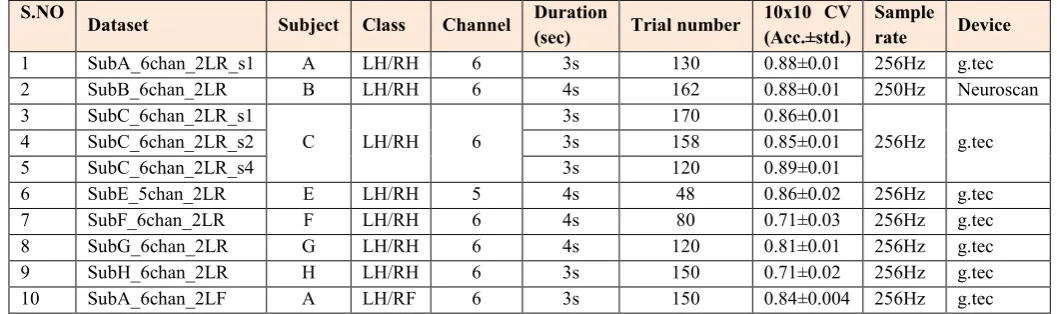
Table 1 provides the information for each data set file including subject ID, motor imagery class, channel number, duration of each imagination task, trial number, sample rate, device name and the 10x10 folder cross validation performance (accuracy ± standard deviation) on this data set. Please note that this performance is roughly obtained by basic preprocess, CSP feature extraction and LDA classifier. The complete same method with same parameters are used to test all data sets without selecting the optimal channels, frequency band and feature number for each subject's data set. Therefore, this results can be used as a general comparison between these data sets and is helpful for understanding which data set is the best and which subject is the best.

Each file is recorded from an experiment which is independent from others. This means we can obtain more data sets with 2-class mental tasks for subject A, B and C by extracting the subset corresponding to the first two classes (left hand & right hand) from 3-class data set of the same subject. Hence, the performance of first two classes is also provided for the 3-class data sets. In Table 1, the column of class denotes the different combination of mental tasks:

 LH/RH: 2 classes of left hand and right hand;  LH/RF: 2 classes of left hand and right foot;

Table 1: The Detail Information of Data Set

S.NO

Dataset Subject Class Channel Duration

(sec) Trial number

10x10 CV (Acc.±std.)

Sample

rate Device

1 SubA_6chan_2LR_s1 A LH/RH 6 3s 130 0.88±0.01 256Hz g.tec

2 SubB_6chan_2LR B LH/RH 6 4s 162 0.88±0.01 250Hz Neuroscan

3 SubC_6chan_2LR_s1

C LH/RH 6

3s 170 0.86±0.01

256Hz g.tec

4 SubC_6chan_2LR_s2 3s 158 0.85±0.01

5 SubC_6chan_2LR_s4 3s 120 0.89±0.01

6 SubE_5chan_2LR E LH/RH 5 4s 48 0.86±0.02 256Hz g.tec

7 SubF_6chan_2LR F LH/RH 6 4s 80 0.71±0.03 256Hz g.tec

8 SubG_6chan_2LR G LH/RH 6 4s 120 0.81±0.01 256Hz g.tec

9 SubH_6chan_2LR H LH/RH 6 3s 150 0.71±0.02 256Hz g.tec

(6)

IV.

FEATURE EXTRACTION

The Haralick Features We extracted features using statistical Haralick feature from the raw EEG data should capture 13 features [19]: Entropy(f1), Energy(f2), Contrast(f3), homogeneity(f4), Inertia(f5), Cluster Prominence(f6),Cluster Shade(f7),Correlation (f8), Autocorrelation(f9), Dissimilarity(f10), Sum of Squares(f11), Sum Entropy(f12), Difference Entropy(f13). The following equation define these features.

Entropy f1 = -∑i ∑j P(i,j)log2( (1)

Energy f2 = ∑i ∑j {P(i,j)}2 (2)

Contrast f3= ∑ ∑ ∑ ₍₃₎

Homogeneity _f4 = ∑i ∑j

P(i,j) (4) Inertia f5= ∑i ∑j (i-j)2 P(i,j) (5)

Cluster Prominence

f6 = ∑i ∑j ((i-µ)+(j-µ))4P(i,j) (6)

Cluster Shade f7 = ∑i ∑j ((i-µ)+(j-µ))3P(i,j) (7)

Correlation _f₈₌∑ ∑ (8)

Autocorrelation f9=∑i ∑j(i.j).p(i,j) (9)

Dissimilarity f10= ∑i ∑j|i-j|.p(i,j) (10)

Sum of Squares f11=∑i ∑j (i-µ)2P(i,j) (11)

Sum Entropy _f12= - ∑ (i)log{Px+y(i)} (12)

Difference Entropy

f13= -∑

(i)log{Px-y(i)} (13)

V.

NORMALIZATION

The normalization procedure[20] can be implemented in different ways. These approaches normalize the data by dividing the attribute value xij by its range using scaling with a shift (the min–max normalization).

Min Max

=

(14)

VI.

FEATURE SELECTION USING FISHER SCORE

Feature selection is a process that aims to identify a small subset of features from a large number of features collected in the data set. Fisher score is one of the simplest filter algorithms for feature selection [21]. In this criteria, the features are selected which have the similar values in the same class and the dissimilar values in different classes. The Fisher score is calculated using the formula.

Where

µi is the mean of the ith features

nj is the number of instances in the jth class

µij and σij are the mean and the variance of the ith

of the features in the jth_{class, respectively.}

VII.

DISCRETIZATION METHODS

The simplest discretization method is called equal-width interval discretization and this method has often been applied as a means for producing nominal values from continuous ones. This approach divides the range of observed values for a feature into k equal sized bins, where k is a parameter provided by the user. The process involves sorting the observed values of a continuous feature and finding the minimum, Vmin and maximum, Vmax, values. The interval Eq. (16)

Fisher Score(FS) _FS₌∑

(7)

can be computed by dividing the range of observed values for the variable into k equally sized bins, where k is a parameter supplied by the user:

Equal width Binning

Interval =

(16)

Boundaries= Vmin+(i×interval)

(17)

and then the boundaries then can be constructed using Eq. (17) where i = 1,..., k-1. This type of discretization does not depend on the multi-relational structure of the data. However, this method of discretization is sensitive to outliers that may drastically skew the range[22] .

VIII.

CLASSIFICATION ALGORITHM

Classification is used to find out in which group each data instance is related within a given dataset. In this study we used three classification algorithm and evaluate the classification performance.

A. Support Vector machine algorithm

The Support Vector Machine(SVM) [23] is a linear discriminant that maximizes the separation between two classes based on the assumption that it improves the classifiers generalization capability. This is achieved by minimizing the cost function

J(W)= ||w||2 ₍₁₈₎

Subject to the constraint

Yi(W’.Xi –b) 1 i=1..n, (19)

Where X1,X2,X3………..Xn are the training data

and b is a bias.

The SVM employs the linear discriminant classification rule given in the equation

{

(20)

Support Vector Machines (SVMs) are the newest supervised machine learning technique (Vapnik, 1995). SVMs revolve around the notion of a “margin” either side of a hyper plane that separates two data classes. Maximizing the margin and thereby creating the largest possible distance between the separating hyper plane and the instances on either side of it has been proven to reduce an upper bound on the expected generalization error.

Algorithm 1: Algorithm for SVMs

1. Introduce positive Lagrange multipliers, one for each of the inequality constraints

2. This gives Lagrangian: 3. LP = | w|2 _–_∑

yi (xi.w-b)+∑ Minimize

LP with respect to w, b.

4. This is a convex quadratic programming problem. 5. In the solution, those points for which αi>0 are

called “support vectors”

B. K-Nearest Neighbor Algorithm:

K-Nearest neighbor algorithm (KNN) is one of the supervised learning algorithms that have been used in many applications in the field of data mining, statistical pattern recognition and many others. It follows a method for classifying objects based on closest training examples in the feature space.[24]

argmaxi∑ (Dj|D)* (C(Dj),i) (21)

One of the most straight forward lazy learning algorithms is the K nearest neighbor algorithm. Lazy-learning algorithms require less computation time during the training phase but more computation time during the classification process.

Algorithm 2: Algorithm for K-Nearest Neighbour

TRAIN- KNN(C,D)

1. D’ ←Preprocess(D)

(8)

3. return D’ ,k

C. The Naive Bayes algorithm

The Naive Bayes algorithm[25] is a simple probabilistic classifier that calculates a set of probabilities by counting the frequency and combinations of values in a given data set. The probability of a specific feature in the data appears as a member in the set of probabilities and is derived by calculating the frequency of each feature value within a class of a training data set. The training dataset is a subset, used to train a classifier algorithm by using known values to predict future, unknown values.

Bayesian classifiers use Bayes theorem which says

P(Cj|D) =

(19)

Where

P(Cj|D) is the probability of instance d being in class

CjP(D|Cj) is the probability of generating instance d

given class Cj

P(Cj) is the probability of occurrence of class Cj

P(D) is the probability of instance d occurring

Algorithm 3:Algorithm for Naïve Bayes

1. Procedure Bayesian_Classifier(X = <X1,,,Xn>):

2. Begin

IX.

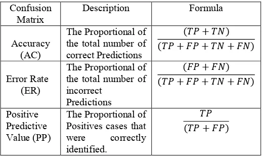
MEASURES OF PERFORMANCE EVALUATION

Different measures are used to evaluate the performance of the system. We used tenfold cross validations and all experiments were repeated 10 times. Confusion Matrix includes information about actual and predicted classifications applied by a classifier. The data in the matrix is using to evaluate the performance of the classifier. In Table 2 shows the confusion matrix for a two class classifier. It includes TN,TP,FP,FN means True Negative, True Positive, False Positive and False Negative respectively.

Table 2: Confusion Matrix

Some of the computational measures from the confusion matrix are tabulated in Table-3.

Table 3: Confusion Matrix Description

(9)

KNN SVM NAIVE BAYES

(Sen) The Proportional of actual positive cases that were

X.

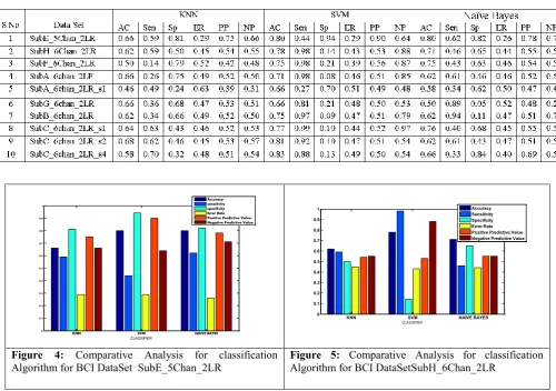
RESULTS AND DISCUSSIONS

The experiment is performed using the BCI Motor imaginary Data Set. Data sets provided by the Dr.Cichocki's Lab (Lab. for Advanced Brain Signal Processing), BSI, RIKEN collaboration with Shanghai Jiao Tong University. In this study we used 10 dataset from BCI data set. If accuracy, specificity and

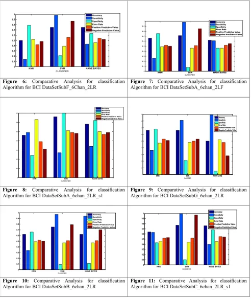
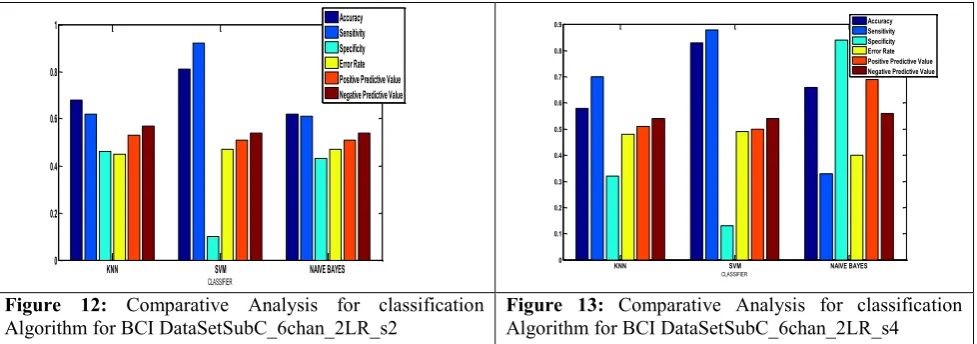
positive predictive becomes high the performance of the classifier is good. If sensitivity, Error Rate and Negative Predictive value becomes low the performance of the classifier is good. Each data set is separately classified by three classification algorithm and analysed the results. The BCI data sets are classified using KNN, SVM, Naïve Bayes classifier. In Table 4. shows the classification measures of three classification algorithms. Figure 4 to 13 shows the classification Performance of the KNN, SVM, Naïve Bayes classifier respectively.

The accuracy values of three classification algorithms such as KNN, SVM, Naïve Bayes is based on the measures SVM classification algorithm shows the highest performance for all the datasets.

T

ABLE

4:

C

LASSIFICATION

M

EASURES

Figure 4: Comparative Analysis for classification

(10)

Algorithm for BCI DataSetSubF_6Chan_2LR Figure 7:Algorithm for BCI DataSetSubA_6chan_2LF Comparative Analysis for classification

Algorithm for BCI DataSetSubA_6chan_2LR_s1 Figure 9:Algorithm for BCI DataSetSubG_6chan_2LR Comparative Analysis for classification

(11)

Algorithm for BCI DataSetSubC_6chan_2LR_s2 Figure 13:Algorithm for BCI DataSetSubC_6chan_2LR_s4 Comparative Analysis for classification

XI.

CONCLUSION

In this paper, We mainly focused on machine learning verdict of EEG signal and performance of the classification algorithm of Naïve Bayes, KNN, SVM using BCI Data set. The results which they obtained or analysed, and compared.in order to provide the readers with guidelines to choose a classifier for a BCI data set. The classification performance of these 10 data sets are tabulated in Table 4. The data set efficiency is evaluated by the means of classification accuracy, sensitivity, specificity, Error Rate, Positive predictive value, Negative Predictive value of three classifiers. Finally we propose the SVM classification algorithm for the BCI data set.

XII.

ACKNOWLEDGEMENT

The author would like to thank to Dr.Cichocki's Lab (Lab. for Advanced Brain Signal Processing), BSI, RIKEN collaboration with Shanghai Jiao Tong University, for providing BCI data-set.

XIII.

REFERENCES

[1]

Q.B. Zhao, L.Q. Zhang, C. Andrzej J. Li,” Incremental common spatial pattern algorithm for BCI”, in: Proceedings of the International Joint Conference on Neural Networks, 2008, pp. 2656–2659.

[2]

M.A. Oskoei, J.Q. Gan, Huosheng Hu, “Adaptive schemes applied to online SVM for BCI data classification”, in: Proceedings of the 31st Annual International Conference of the IEEE EMBS, 2009, pp. 2600–2603.

[3]

C.Vidaurre, M. Kawanabe1, P. von Bunau, B. Blankertz, K.R. Muller, “Toward an ¨unsupervised adaptation of LDA for brain– computer interfaces, IEEE Trans. Biomed. Eng 58 (3) (2011) 587–597.

[4]

C.S.L. Tsui, J.Q. Gan, Comparison of three methods for adapting LDA classifiers with BCI applications, in: Proceedings of the 4th International Workshop on Brain–Computer Interfaces, Graz, Austria, 2008, pp. 116–121.

[5]

C.S.L. Tsui , J.Q. Gan, Asynchronous BCI control of a robot simulator with supervised online training, in: Proceedings of the International Conference on Intelligent Data Engineering and Automated Learning, IDEAL, 2007, Birmingham, UK, pp. 125–134.

0 0.2 0.4 0.6 0.8 1

CLASSIFIER

Accuracy Sensitivity Specificity Error Rate Positive Predictive Value Negative Predictive Value

0 0.1 0.2 0.3 0.4 0.5 0.6 0.7 0.8 0.9

CLASSIFIER

(12)

[6]

B. Grychtol, H. Lakany, G. Valsan, et al., “Human behavior integration improves classification rates in real-time BCI”, IEEE Trans. Neural. Syst. Rehabil. Eng. 18 (4) (2010) 362–368.

[7]

J.W. Yoon, S.J. Roberts, M. Dyson“Adaptive classification for brain computer interface systems using sequential Monte Carlo sampling, Neural”. Net. 22 (2009) 1286- 1294.

[8]

D.S. Huang,”Systematic Theory of Neural Networks for Pattern Recognition”, Publishing House of Electronic Industry of China, Beijing, 1996.

[9]

D.S.Huang,”Radial basis probabilistic neural networks: model and application”, Int. J. Pattern Recognition Artif. Intell. 13 (7) (1999) 1083–1101.

[10]

D.S. Huang, J.X. Du,”A constructive hybrid structure optimization methodology for radial basis probabilistic neural networks”, IEEE. Trans. Neural Networks 19 (12) (2008) 2099– 2115.

[11]

M.K. Hazrati, A. Erfanian, “An online EEG-based brain–computer interface for controlling hand grasp using an adaptive probabilistic neural network”, Med. Eng. Phys. 32 (2010) 730–739.

[12]

P. Shenoy, M. Krauledat, B. Blankertz, Rajesh P.N. Rao, K.R. Muller, “Towards adaptive classification for BCI”, J. Neural. Eng. 3 (2006) 13–23.

[13]

S.L. Sun, Y. Lu, Y.G. Chen,”The stochastic approximation method for adaptive Bayesian classifiers: towards online brain–computer interfaces”, Neuro. Comput. Appl. 20 (2011) 31– 40.

[14]

MihaelaMaracine, Alexandra Radu, VlaCiobanu, Nirvana Popescu ,” Brain Computer Interface Architectures and Classification Approaches”, 21st International

Conference on Control Systems and Computer Science,2017.

[15]

Lotte, L Bougrain, A Cichocki, M Clerc, M Congedo, A Rakotomamonjy, and F Yger“A Review of Classification Algorithms for EEG-based Brain Computer Interfaces” , Author submitted manuscript - JNE-102129.R1,2018.

[16]

Yongkoo Park, Wonzoo Chung ” BCI Classification using locally generated CSP features”Published on Jan 2018 6th International Conference on Brain-Computer Interface (BCI).

[17]

Keum-ShikHong , M. Jawad Khan and Melissa J. Hong, “Feature Extraction and Classification Methods for Hybrid fNIRS-EEG Brain-Computer Interfaces”, published on 28 June 2018 Volume 12 , Article 246.

[18]

HardikMeisheri, NagarajRamrao, Suman K. Mitra,” Multiclass Common Spatial Pattern for EEG based Brain Computer Interface with Adaptive Learning Classifier”,25 Feb 2018.

[19]

R.M.Haralick, K.Shanmugam, and I.Dinstein, “Texture features for image classification”, IEEE Trans.Syst.Man.Cybernetics, vol SMC-3, pp. 610-621, 1973.

[20]

Dr.C.Velayutham“Non-invasive

electroencephalography signals classification using roughneural network”, Int. J. Computational Biology and Drug Design, Vol. 8, No. 3, 2015.

[21]

V. Arul Kumar, L. Arockiam,” MFSPFA: An Enhanced Filter based Feature Selection Algorithm”, International Journal of Computer Applications (0975 – 8887) Volume 51– No.12, August 2012.

(13)

[23]

Mrs. NaliniJagtap , Mrs. P. P. Shevatekar , Mr. NareshkumarMustary,” A Comparative study of classification techniques in data mining algorithms”, International Journal of Modern Trends in Engineering and Research (IJMTER) Volume 04, Issue 7, [July– 2017]ISSN (Online):2349–9745; ISSN (Print):2393- 8161.

[24]

George Dimitoglou, JamesA. Adams, and Carol M. Jim,”Comparison of the C4.5 and a Naïve Bayes Classifier for the Prediction of Lung Cancer Survivability” Journal of Computing, Volume 4, Issue 8, 2012.

[25]

Kai KengAng, Zheng Yang Chin, Haihong Zhang and Cuntai Guan,” Filter Bank Common Spatial Pattern (FBCSP) in Brain – Computer Interface” 2008 International Joint Conference on Neural Networks(IJCNN 2008).

Cite this article as :