CSEIT1833189 | Received : 15 March 2018 | Accepted : 29 March 2018 | March-April-2018 [ (3 ) 3 : 262-269 ]
© 2018 IJSRCSEIT | Volume 3 | Issue 3 | ISSN : 2456-3307
306
Prediction of Heart Diseases Using Data Mining and Machine
Learning Algorithms and Tools
M. Nikhil Kumar, K. V. S. Koushik, K. Deepak
Department of CSE, VR Siddhartha Engineering College, Vijayawada, Andhra Pradesh, India
ABSTRACT
Data mining is the most popular knowledge extraction method for knowledge discovery (KDD). Machine learning is used to enable a program to analyze data, understand correlations and make use of insights to solve problems and/or enrich data and for prediction. Data mining techniques and machine learning algorithms play a very important role in medical area. The health care industry contains a huge amount of data. But most of it is not effectively used. Heart disease is one of the main reason for death of people in the world. Nearly 47% of all deaths are caused by heart diseases. We use 8 algorithms including Decision Tree, J48 algorithm, Logistic model tree algorithm, Random Forest algorithm, Naïve Bayes, KNN, Support Vector Machine, Nearest Neighbour to predict the heart diseases. Accuracy of the prediction level is high when using more number of attributes. Our aim is to perform predictive analysis using these data mining, machine learning algorithms on heart diseases and analyze the various mining, Machine Learning algorithms used and conclude which techniques are effective and efficient.
Keywords: Data Mining, Machine Learning, Decision Tree, Heart Disease.
I.
INTRODUCTION
The heart is the hardest working muscle in the body. The average heart beats 100,000 times a day, day and night, to supply oxygen and nutrients throughout the body. Blood pumped by the heart also shuttles waste products such as carbon dioxide to the lungs so it can be eliminated from the body. Proper heart function is essential to support life. Coronary artery disease (CAD), commonly known as heart disease, is a condition in which cholesterol, calcium, and other fats accumulate in the arteries that supply blood to the heart. This material hardens forming a plaque that blocks blood flow to the heart. When a coronary artery narrows due to plaque build up or some other cause, the heart muscle is starved for oxygen and a person experiences chest pain known as angina.
1.1 BACKGROUND
Millions of people are getting some sort of heart disease every year and heart disease is the biggest killer of both men and women in the United States and around the world. The World Health Organization (WHO) analyzed that twelve million deaths occurs worldwide due to Heart diseases. In almost every 34 seconds the heart disease kills one person in world.
heart disease helps medicinal services experts to recognize patients at high risk of having Heart disease. Statistical analysis has identified risk factors associated with heart disease to be age, blood pressure, total cholesterol, diabetes, hyper tension, family history of heart disease, obesity and lack of physical exercise, fasting blood sugar etc [3].
1.2 DATA MINING
Data mining is the process of discovering patterns in large data sets involving methods at the intersection of machine learning, statistics, and database systems. It is an essential process where intelligent methods are applied to extract data patterns [2]. The Data mining may be accomplished using classification, clustering, prediction, association and time series analysis.
Data mining is the exploration of large datasets to extract hidden and previously unknown patterns, relationships and knowledge that are difficult to detect with traditional statistical methods (Lee, Liao et al. 2000). Thus data mining refers to mining or extracting knowledge from large amounts of data. Data mining applications will be used for better health policy-making and prevention of hospital errors, early detection, prevention of diseases and preventable hospital deaths (Ruben 2009). Heart disease prediction system can assist medical professionals in predicting heart disease based on the clinical data of patients [1]. Hence by implementing a heart disease prediction system using Data Mining techniques and doing some sort of data mining on various heart disease attributes, it can able to predict more probabilistically that the patients will be diagnosed with heart disease. This paper presents a new model that enhances the Decision Tree accuracy in identifying heart disease patients. It uses the different algorithm of Decision Trees.
We use Waikato Environment for Knowledge Analysis (WEKA).The information of UCI repository regularly introduced in a database or spreadsheet. In
Vijiyaraniet. al. [2] performed a work, An Efficient Classification Tree Technique for Heart Disease Prediction. This paper analyzes the classification tree techniques in data mining. The classification tree algorithms used and tested in this paper are Decision Stump, Random Forest and LMT Tree algorithm. The objective of this research was to compare the outcomes of the performance of different classification techniques for a heart disease dataset. A novel technique to develop the multi-parametric feature with linear and nonlinear characteristics of HRV (Heart Rate Variability) was proposed by Heon Gyu Lee et al. [9]. Statistical and classification techniques were utilized to develop the multiparametric feature of HRV. Besides, they have assessed the linear and the non-linear properties of HRV for three recumbent positions, to be precise the supine, left lateral and right lateral position. Numerous experiments were conducted by them on linear and nonlinear characteristics of HRV indices to assess several classifiers such as Bayesian classifiers, CMAR (Classification based on Multiple Association Rules), C4.5 (Decision Tree) and SVM (Support Vector Machine). SVM surmounted the other classifiers.
III. HEART DISEASE
The term Heart sickness alludes to illness of heart & vessel framework inside it. Heart illness is a wide term that incorporates different sorts of sicknesses influencing diverse segments of the heart. Heart signifies "cardio." Therefore, all heart sicknesses fit in with the class of cardiovascular ailments.
3.1 SYMPTOMS
The most common symptom of coronary artery disease is angina, or chest pain. Angina can be described as a discomfort, heaviness, pressure, aching, burning, fullness, squeezing, or painful feeling in your chest. It can be mistaken for indigestion or heartburn. Angina may also be felt in the shoulders, arms, neck, throat, jaw, or back.
Other symptoms of coronary artery disease include:
Shortness of breath
Palpitations (irregular heart beats, or a "flip-flop" feeling in your chest)
Manifestations of a heart assault can include:
Discomfort, weight, largeness, or agony in the midsection, arm, or beneath the breastbone.
Discomfort emanating to the back, jaw, throat, or arm.
Fullness, heartburn, or stifling feeling (may feel like indigestion).
Sweating, queasiness, heaving, or unsteadiness.
Extreme shortcoming, nervousness, or
shortness of breath.
Rapid or not regular heart beats
3.3 TYPES OF HEART DISEASES
Arrhythmia is an irregular or abnormal heartbeat. This can be a slow heart beat (bradycardia), a fast heartbeat (tachycardia), or an irregular heartbeat. Some of the most common arrhythmias include atrial fibrillation (when the atria or upper heart chambers contract irregularly), premature ventricular contractions (extra beats that originate from the lower heart chambers, or ventricles), and bradyarrhythmias (slow heart rhythm caused by disease of the heart's conduction system).
Heart failure (congestive heart failure, or CHF) occurs when the heart is not able to pump sufficient oxygen-rich blood to meet the needs of the rest of the body. This may be due to lack of force of the heart to pump or as a result of the heart not being able to fill with enough blood. Some people have both problems.
Heart valve disease occurs when one or more of the four valves in the heart are not working properly. Heart valves help to ensure that the blood being pumped through the heart keeps flowing forward. Disease of the heart valves (e.g., stenosis, mitral valve prolapse) makes it difficult.
Heart muscle disease (cardiomyopathy) causes the heart to become enlarged or the walls of the heart to become thick. This causes the heart to be less able to pump blood throughout the body and often results in heart failure.
Congenital heart disease is a type of birth defect that causes problems with the heart at birth and occurs in about one out of every 100 live births. Some of the most common types of congenital heart disease include:
atrial septal defects (ASD) and ventricular septal defects (VSD), which occur when the walls that separate the right and left chambers of the hearts are not completely closed.
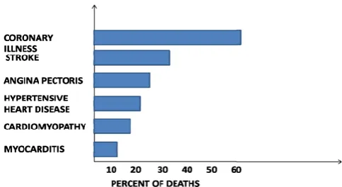
Figure 1. Different causes of Heart Diseases
IV. WEKA TOOL
We use WEKA (www.cs.waikato.ac.nz/ml/weka/), an open source data mining tool for our experiment. [9]WEKA is developed by the University of Waikato in New Zealand that implements data mining algorithms using the JAVA language. WEKA is a state-of-the-art tool for developing machine learning (ML) techniques and their application to real-world data mining problems. It is a collection of machine learning algorithms for data mining tasks. The algorithms are applied directly to a dataset. WEKA implements algorithms for data preprocessing, feature reduction, classification, regression, clustering, and association rules. It also includes visualization tools. The new machine learning algorithms can be used with it and existing algorithms can also be extended with this tool. Main Features
49 data preprocessing tools
76 classification/regression algorithms
8 clustering algorithms
3 algorithms for finding association rules
15 attribute/subset evaluators + 10 search algorithms for feature selection
Main GUI
Three graphical user interfaces
“The Explorer” (exploratory data analysis)
“The Experimenter” (experimental
environment)
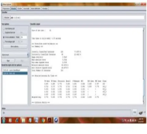
Figure 2. WEKA
We have applied following five commonly used classifiers for prediction on the basing on their performance. These classifiers are as follows:
Table 1. Commonly used Algorithms
Generic Name WEKA Name
Bayesian Network Naïve Bayes(NB)
Support Vector Machine SMO
C4.5 Decision Tree J48
K-Nearest Neighbour 1Bk
4.1 DATA DESCRIPTION
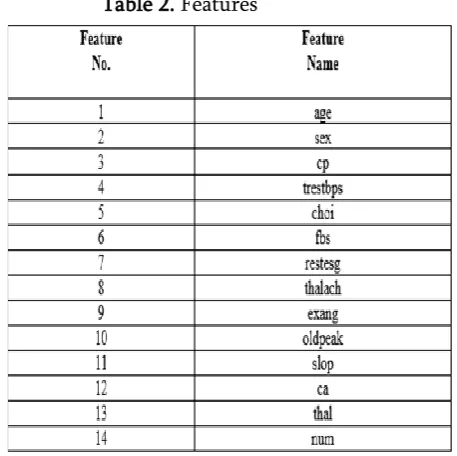
We performed computer simulation on one dataset. Dataset is a Heart dataset. The dataset is available in UCI Machine Learning Repository [10]. Dataset contains 303 samples and 14 input features as well as 1 output feature. The features describe financial, personal, and social feature of loan applicants. The output feature is the decision class which has value 1 for Good credit and 2 for Bad credit. The dataset-1 contains 700 instances shown as Good credit while 300 instances as bad credit. The dataset contains features expressed on nominal, ordinal, or interval scales. A list of all those features is given in Table 1.
Table 2. Features
Table 3. Selected Heart Disease Attributes
4.2 DECISION TREE
control statements. These are a non-parametric
supervised learning method used for classification
and regression. The goal is to create a model that predicts the value of a target variable by learning simple decision rules inferred from the data features. Decision trees can handle both numerical data and categorical data. For medical purpose, decision trees determine order in different attributes and decision is taken based on the attribute.
A Decision Tree is used to learn a classification function which concludes the value of a dependent attribute (variable) given the values of the independent (input) attributes. This verifies a problem known as supervised classification because the dependent attribute and the counting of classes (values) are given [4]. Tree complexity has its effect on its accuracy. Usually the tree complexity can be measured by a metrics that contains: the total number of nodes, total number of leaves, depth of tree and number of attributes used in tree construction. Tree size should be relatively small that can be controlled by using a technique called pruning [5].
The three decision tree algorithms namely J48 algorithm, logistic model tree algorithm and Random Forest decision tree algorithm are used for comparison. The proposed methodology involves reduced error pruning, confident factor and seed parameters to be considered in the diagnosis of heart disease patients. Reduced error pruning has shown to drastically improve decision tree performance. These three decision tree algorithms are then tested to identify which combination will provide the best performance in diagnosing heart disease patients. Training => Algorithm => Model => Testing => Evaluation
Advantages:
1) Understandable prediction rules are created from the training data.
2) Builds the fastest tree. 3) Builds a short tree.
4) Only need to test enough attributes until all data is classified.
Disadvantages:
1) Data may be over fitted or over classified. 2) Only one attribute at a time is tested for making
decision.
Figure 3. Decision Tree 4.3 J 48
J48 is a Decision tree that is an implementation of ID3 (Iterative Dichtomiser 3) developed by the WEKA project team. R language also has a package to implement this. J48 does not require discretization of numeric attributes. Classifiers, like filters, are organized in a hierarchy: J48 has the full name weka.classifiers.trees.j48. The classifier is shown in the text box next to choose button: It reads J48 –C 0.25 –M 2. This text gives the default parameter settings for this classifier. The additional features of J48 are accounting for missing values, decision trees
pruning, continuous attribute value ranges,
derivation of rules, etc. This algorithm it generates the rules from which particular identity of that data is generated. The objective is progressively generalization of a decision tree until it gains equilibrium of flexibility and accuracy.
Advantages:
based on what is known about the attribute values for the other records.
2) In case of potential over fitting pruning can be used as a tool for précising.
Disadvantages:
1) Size of J48 trees which increases linearly with the number of examples.
2) J48 rules slow for large and noisy datasets.
3) Space Complexity is very large as we have to store the values repeatedly in arrays.
4.4 J48 WITH REDUCED ERROR PRUNING
Pruning is very important technique to be used in tree creation because of outliers. It also addresses overfitting. Datasets may contain little subsets of instances that are not well defined. To classify them correctly, pruning can be used. Separate and Conquer rule learning algorithm is basis to prune any tree. This rule learning scheme starts with an empty set of rules and the full set of training instances. Reduced-error pruning is one of such separate and conquer rule learning scheme. There are two types of pruning i.e.
1) Post pruning (performed after creation of tree) 2) Online pruning (performed during creation of tree).
After extracting the decision tree rules, reduced error pruning was used to prune the extracted decision rules. Reduced error pruning is one of the fastest pruning methods and known to produce both accurate and small decision rules (Esposito, Malerba et al. 1997). Applying reduced error Pruning provides more compact decision rules and reduces the number of extracted rules.
4.5 LOGISTIC MODEL TREE ALGORITHM
A logistic model tree basically consists of a standard decision tree structure with logistic regression functions at the leaves, much like a model tree is a regression tree with regression functions at the leaves. As in ordinary decision trees, a test on one of the attributes is associated with every inner node. For a
nominal (enumerated) attribute with k values, the node has k child nodes, and instances are sorted down one of the k branches depending on their value of the attribute. For numeric attributes, the node has two child nodes and the test consists of comparing the attribute value to a threshold: an instance is sorted down the left branch if its value for that attribute is smaller than the threshold and sorted down the right branch otherwise.
More formally, a logistic model tree consists of a tree structure that is made up of a set of inner or non-terminal nodes N and a set of leaves or non-terminal nodes T. Let S = D1 ×···× Dm denote the whole instance space, spanned by all attributes V = {v1,...,vm} that are present in the data. Then the tree structure gives a disjoint subdivision of S into regions St , and every region is represented by a leaf in the tree:
Unlike ordinary decision trees, the leaves t ∈ T have an associated logistic regression function ft instead of just a class label. The regression function ft takes into account an arbitrary subset Vt ⊂ V of all attributes present in the data, and models the class membership probabilities as
Note that both standalone logistic regression and dataset in question: for small datasets where a simple linear model offers the best bias-variance trade off, the logistic model „tree‟ should just consist of a single logistic regression model, i.e. be pruned back to the root. For other datasets, a more elaborate tree structure is adequate.
To construct a logistic model tree by developing a standard classification tree, building logistic regression models for all node, pruning a percentage of the sub-trees utilizing a pruning model, and combining the logistic models along a way into a solitary model in some manner is performed.
The pruning plan uses cross-validation to get more steady pruning results. In spite of the fact that this expanded the computational multifaceted nature, it brought about littler and for the most part more accurate trees. These thoughts lead to the following algorithm for developing logistic model trees:
Tree developing begins by building a logistic model at the root utilizing the LogitBoost algorithm. The quantity of cycles (and basic relapse capacities fmj to add to Fj) is resolved utilizing 10 fold cross-validation. In this process the information is part into preparing and test set 10 times, for each preparation set LogitBoost is rush to a greatest number of cycles and the lapse rates on the test set are logged for each cycle and summed up over the distinctive folds. The quantity of emphases that has the least whole of blunders is utilized to prepare the LogiBoost algorithm on all the information. This gives the logistic regression model at the base of the tree.
4.6 RANDOM FOREST ALGORITHM
Random forest algorithm is a supervised classification algorithm. As the name suggest, this algorithm creates the forest with a number of trees.
In general, the more trees in the forest the more robust the forest looks like. In the same way in the random forest classifier, the higher the number of trees in the forest gives the high accuracy results.
There are three methodologies for Random Forest, for example, Forest-RI(Random Input choice) and Forest-RC (Random blend) and blended of Forest-RI and Forest-RC. choose aside from the quantity of indicators to pick at arbitrary at every node.
It runs effectively on extensive databases; it is
moderately strong to anomalies and
commotion.
It can deal with a huge number of information variables without variable deletion; it gives evaluations of what variables are important in classification.
It has a successful system for assessing missing information and keeps up accuracy when a vast extent of the data are missing, it has methods for adjusting error in class populace unequal data sets.
Advantages:
1) The same random forest algorithm or the random forest classifier can use for both classification and the regression task.
2) Random forest classifier will handle the missing values.
4) Can model the random forest classifier for categorical values also.
Disadvantages:
1) Quite slow to create predictions once trained. More accurate ensembles require more trees, which means using the model becomes slower.
2) Results of learning are incomprehensible. Compared to a single decision tree, or to a set of rules, they don't give you a lot of insight.
4.7 NAÏVE BAYES CLASSIFIER
This classifier is a powerful probabilistic representation, and its use for classification has received considerable attention. This classifier learns from training data the conditional probability of each attribute Ai given the class label C. Classification is then done by applying Bayes rule to compute the probability of C given the particular instances of A1…..An and then predicting the class with the highest posterior probability. The goal of classification is to correctly predict the value of a designated discrete class variable given a vector of predictors or attributes. In particular, the Naive Bayes classifier is a Bayesian network where the class has no parents and each attribute has the class as its sole parent. Although the naive Bayesian (NB) algorithm is simple, it is very effective in many real world datasets because it can give better predictive accuracy than well known methods like C4.5 and BP [11],[12] and is extremely efficient in that it learns in a linear fashion using ensemble mechanisms, such as bagging and boosting, to combine classifier predictions [13]. However, when attributes are redundant and not normally distributed, the predictive accuracy is reduced
Advantages:
1) Easy to implement.
2) Requires a small amount of training data to estimate the parameters.
3) Good results obtained in most of the cases.
Disadvantages:
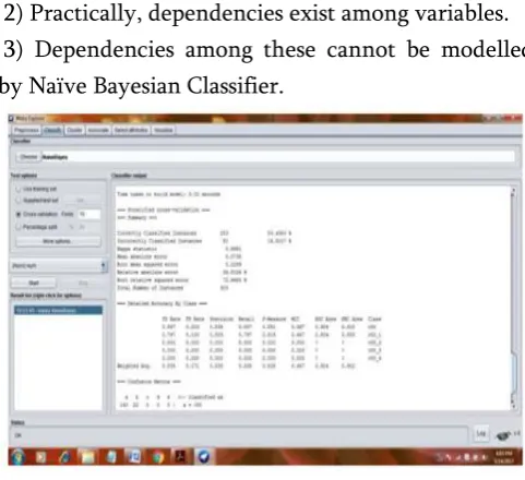
1) Assumption: class conditional independence, therefore loss of accuracy.
2) Practically, dependencies exist among variables. 3) Dependencies among these cannot be modelled by Naïve Bayesian Classifier.
Figure 4. Naïve Bayes Classifier
4.8 K-NEAREST NEIGHBOUR
This classifier is considered as a statistical learning algorithm and it is extremely simple to implement and leaves itself open to a wide variety of variations. In brief, the training portion of nearest-neighbour does little more than store the data points presented to it. When asked to make a prediction about an unknown point, the nearest-neighbour classifier finds the closest training-point to the unknown point and predicts the category of that training point according to some distance metric. The distance metric used in nearest neighbour methods for numerical attributes can be simple Euclidean distance.
4.9 SUPPORT VECTOR MACHINE
Support vector machines exist in different forms, linear and non-linear. A support vector machine is a supervised classifier. What is usual in this context, two different datasets are involved with SVM, training and a test set. In the ideal situation the classes are linearly separable. In such situation a line can be found, which splits the two classes perfectly. However not only one line splits the dataset perfectly, but a whole bunch of lines do. From these lines the best is selected as the "separating line". The best line is found by maximizing the distance to the nearest points of both classes in the training set. The maximization of this distance can be converted to an equivalent minimization problem, which is easier to solve. The data points on the maximal margin lines are called the support vectors. Most often datasets are not nicely distributed such that the classes can be separated by a line or higher order function. Real datasets contain random errors or noise which creates a less clean dataset. Although it is possible to create a model that perfectly separates the data, it is not desirable, because such models are over-fitting on the training data. Overfitting is caused by incorporating the random errors or noise in the model. Therefore the model is not generic, and makes significantly more errors on other datasets. Creating simpler models keeps the model from over-fitting. The complexity of the model has to be balanced between fitting on the training data and being generic. This can be achieved by allowing models which can make errors. A SVM can make some errors to avoid over-fitting. It tries to minimize the number of errors that will be made. Support vector machines classifiers are applied in many applications. They are very popular in recent research. This popularity is due to the good overall empirical performance. Comparing the naive Bayes and the SVM classifier, the SVM has been applied the most[15].
Figure 6. SVM
V.
PERFORMANCE COMPARISONS &
RESULTS
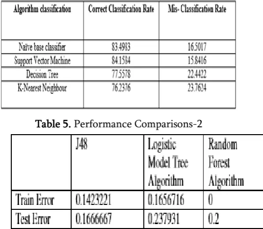
Table 4. Performance Comparisons-1
Table 5. Performance Comparisons-2
Also, J48 algorithm utilization reduced-error pruning form less number of trees. The LMT algorithm manufactures the littlest trees. This could show that cost-many-sided quality pruning prunes down to littler trees than decreased lapse pruning, yet it additionally demonstrate that the LMT algorithm does not have to assemble huge trees to group the information. The LMT algorithm appears to perform better on data sets with numerous numerical attributes, while for good execution for3 algorithm, the data sets with couple of numerical qualities gave a superior execution. We can see from the outcomes thatJ48 is the best classification tree algorithm among the three with pruning system.
VI. CONCLUSION
Finally, we carried out an experiment to find the predictive performance of different classifiers. We select four popular classifiers considering their qualitative performance for the experiment. We also choose one dataset from heart available at UCI machine learning repository. Naïve base classifier is the best in performance. In order to compare the classification performance of four machine learning algorithms, classifiers are applied on same data and results are compared on the basis of misclassification and correct classification rate and according to experimental results in table 1, it can be concluded that Naïve base classifier is the best as compared to Support Vector Machine, Decision Tree and K-Nearest Neighbour. After analyzing the quantitative data generated from the computer simulations, Moreover their performance is closely competitive showing slight difference. So, more experiments on several other datasets need to be considered to draw a more general conclusion on the comparative performance of the classifiers.
By analyzing the experimental results, it is concluded thatJ48 tree technique turned out to be best classifier for heart disease prediction because it contains more accuracy and least total time to build. We can clearly
see that highest accuracy belongs to J48 algorithm with reduced error pruning followed by LMT and Random Forest algorithm respectively. Also observed that applying reduced error pruning to J48 results in higher performance while without pruning, it results in lower Performance. The best algorithm J48 based on UCI data has the highest accuracy i.e. 56.76% and the total time to build model is 0.04 seconds while LMT algorithm has the lowest accuracy i.e 55.77% and the total time to build model is 0.39seconds.
In conclusion, as identified through the literature review, we believe only a marginal success is achieved in the creation of predictive model for heart disease patients and hence there is a need for combinational and more complex models to increase the accuracy of predicting the early onset of heart disease.
VII.
REFERENCES
[1]. Prerana T H M1, Shivaprakash N C2 , Swetha N3 "Prediction of Heart Disease Using Machine
Learning Algorithms- Naïve
Bayes,Introduction to PAC Algorithm, Comparison of Algorithms and HDPS" International Journal of Science and Engineering Volume 3, Number 2 – 2015 PP: 90-99 ©IJSE Available at www.ijse.org ISSN: 2347-2200
[2]. B.L Deekshatulua Priti Chandra "Classification of Heart Disease Using K- Nearest Neighbor and Genetic Algorithm " M.Akhil jabbar* International Conference on Computational Intelligence: Modeling Techniques and Applications (CIMTA) 2013.
[3]. Michael W.Berry et.al,"Lecture notes in data mining",World Scientific(2006)
[4]. S. Shilaskar and A. Ghatol, "Feature selection for medical diagnosis : Evaluation for cardiovascular diseases," Expert Syst. Appl., vol. 40, no. 10, pp. 4146–4153, Aug. 2013.
quality of dermatologic diagnosis," Expert Syst. Appl., vol. 36, no. 2, Part 2, pp. 4035–4041, Mar. 2009.
[6]. A. T. Azar and S. M. El-Metwally, "Decision tree classifiers for automated medical diagnosis," Neural Comput. Appl., vol. 23, no. 7–8, pp. 2387–2403, Dec. 2013. 10Y. C. T. Bo Jin, "Support vector machines with genetic fuzzy feature transformation for biomedical data classification.," Inf Sci, vol. 177, no. 2, pp. 476–489, 2007.
[7]. N. Esfandiari, M. R. Babavalian, A.-M. E. Moghadam, and V. K. Tabar, "Knowledge discovery in medicine: Current issue and future trend," Expert Syst. Appl., vol. 41, no. 9, pp. 4434–4463, Jul. 2014.
[8]. A. E. Hassanien and T. Kim, "Breast cancer MRI diagnosis approach using support vector machine and pulse coupled neural networks," J. Appl. Log., vol. 10, no. 4, pp. 277–284, Dec. 2012.
[9]. Sanjay Kumar Sen 1, Dr. Sujata Dash 21Asst. Professor, Orissa Engineering College, Bhubaneswar, Odisha – India.
[10]. UCI Machine Learning Repository, Available at http://archive.ics.uci.edu/ml/machinelearningd atabases/ statlog/german/
[11]. Domingos P and Pazzani M. "Beyond Independence: Conditions for the Optimality of the Simple Bayesian Classifier", in Proceedings of the 13th Conference on Machine Learning, Bari, Italy, pp105-112, 1996.
[12]. Elkan C. "Naive Bayesian Learning, Technical Report CS97-557", Department of Computer Science and Engineering, University of California, San Diego, USA, 1997.
[13]. B.L Deekshatulua Priti Chandra "Reader, PG
Dept. Of Computer Application North Orissa University, Baripada, Odisha – India. "Empirical Evaluation of Classifiers‟ Performance Using Data Mining Algorithm" International Journal of C omputer Trends and
Technology (IJCTT) – Volume 21 Number 3 –
Mar 2015 ISSN: 2231-2803