UCD GEARY INSTITUTE
DISCUSSION PAPER SERIES
Class size effects: evidence using a new
estimation technique
Kevin Denny School of Economics, University College Dublin
Veruska Oppedisano Department of Economics,
University College London Geary WP2010/51
December 2, 2010
UCD Geary Institute Discussion Papers often represent preliminary work and are circulated to encourage discussion. Citation of such a paper should account for its provisional character. A revised version may be available directly from the author.
Any opinions expressed here are those of the author(s) and not those of UCD Geary Institute. Research published in this series may include views on policy, but the institute itself takes no institutional policy positions.
Class size effects: evidence using
a new estimation technique
*Kevin Denny Veruska Oppedisano
School of Economics
University College Dublin
Department of Economics
University College London
December 2
nd2010
Abstract:
This paper estimates the marginal effect of class size on
educational attainment of high school students. We control for the
potential endogeneity of class size in two ways using a
conventional instrumental variable approach, based on changes in
cohort size, and an alternative method where identification is based
on restriction on higher moments. The data is drawn from the
Program for International Student Assessment (PISA) collected in
2003 for the United States and the United Kingdom. Using either
method or the two in conjunction leads to the conclusion that
increases in class size lead to improvements in student’s
mathematics scores. Only the results for the United Kingdom are
statistically significant.
Keywords: class sizes, educational production,
* Corresponding author: Veruska Oppedisano, Department of Economics, University College London,
Gower Street, WC1E 6BT. [email protected]. Veruska Oppedisano acknowledges the generous support of the Marie Curie Excellence Grant FP-6 51706 "Youth Inequalities" whilst based at the Geary Institute. Kevin Denny is affiliated to the UCD Geary Institute and the Institute for Fiscal Studies, London. He thanks the Department of Economics, University of Kentucky for its hospitality. The authors thank Chris Jepsen and seminar participants at the UCD Geary Institute for comments.
1
1. Introduction
Many educationalists, economists, policy makers and the public generally believe that school quality is important1. However knowing exactly what makes a “good school” is far from straightforward. There are several major issues to be addressed in measuring the determinants of school quality. The most obvious one perhaps is data. Unless something is measured one cannot hope to quantify its effects (though one may be able control for its effects in certain circumstances). This is particularly an issue for educational production as schools are, most likely, complex institutions depending on many inputs so that simplistic production functions are unlikely to be informative. That said, the data available to researchers has improved significantly in recent decades particularly with the publication of data from international student assessments such as the Program for Student Assessment (PISA) and the Trends in International Mathematics and Science Study (TIMSS). Perhaps the more challenging issue is the extent to which these and other datasets allow us to specifically measure causal relationships.
The basic problem, well known to economists though perhaps not as widely appreciated elsewhere, is the inputs in educational productions may well not be exogenously determined. The effect of class size on educational outcomes has been at the centre of the debate because of the ambiguous and controversial results of the causal nexus found in the economics literature.
The size of the class that a student is in may depend on choices made by administrators, teachers and parents and may be related to the level of performance achieved by the students, so that observed class sizes may not be exogenous to student performance. For example, parents who care about school quality may be willing to move home and pay higher houses prices to ensure that their children are taught in schools with relatively small classes; also, they might pressure school administrator to place their children in small classes according to their educational needs; similarly, the school system as a whole might allocate students in classes on the basis of their achievement. What this means is that the right hand side variables will be correlated with the disturbance term
1 For recent estimates of the large macroeconomic benefits of improving educational attainment see
2
and hence ordinary least square estimates of school quality effects will be biased and inconsistent.
There are two basic approaches to overcoming this endogeneity bias. The first one is to perform an explicit class-size experiment, where students are randomly assigned to classes of different size in order to guarantee exogeneity of the class-size variation. The second option consists in exploiting exogenous variations in class size, implementing quasi-experimental identification strategies.
Since the mid-1960s, a large literature has unfolded in the United States that tries to estimate the effects of class size on students’ achievement using both approaches. Although extensive reviews of this literature exist, there is much controversy on effectiveness of class-size reductions (see Hanushek, 2003 and Krueger, 2003). Among influential experimental studies, Krueger (1999) evaluates the effects of the large scale STAR experiment in which 11,600 students and their teachers were randomly assigned to small- and regular-size classes during the first four years of school. Findings indicate that students who were randomly assigned to classes with about 12 students performed better than those who were assigned to classes with about 22 students.
A quasi-experimental setting using instrumental variables technique has been used by Hoxby (2000). She exploits variation in class size that comes from population variation to estimate the impact of class size on test scores of pupils enrolled in elementary schools in Connecticut. She finds that class size reduction has no effect on students’ test scores, neither in schools with a high concentration of low income students. These results, in contrast with those found by Krueger, may be explained by the fact that the “Hawthorne effect”2 had played a role in the experimental setting of the STAR project. There are also several studies on educational production in developing countries. Among the more rigorous, Angrist and Levy (1999) use the Maimonides rule as an exogenous source of variation in class size to estimate the effect of class size on schooling achievement of Israeli pupils. They find that smaller class size induces a significant positive impact in test scores for forth and fifth graders, although the
2
The effect refers to the fact that agents involved in the experiment are aware of it and they might change their behaviour when they are being evaluated. One should expect that individuals increase their effort during the evaluation period, making policies appear to have productivity effects that they would not have otherwise. Although if individuals are aware they are in the control group their behaviour could also be affected.
3
estimated effects are mostly smaller than those reported in the Tennessee Star experiment. Case and Deaton (1999) examine the relationship between educational inputs and school outcomes in South Africa before the end of apartheid government, characterized by several limitations of black households on residential choices and funding decisions. The results show that pupil teacher ratio does not affect comprehensive scores of students between thirteen and eighteen of age and has a negative effect on math score significant at 10 percent.
In Europe, there is much less evidence compared to the US. The evidence on the United Kingdom tends to find small effects of class size on educational outcomes (Feinstein and Symons, 1999, Dolton and Vignoles, 1999, Dearden et al., 2002 and Dustmann et al., 2003). Evidence on the effects of class size in continental European countries is provided by Woessman and West (2006). They exploit a combination of fixed effects and an IV strategy to assess the effect of class size on math scores of thirteen aged students from all over the world using the TIMSS dataset. In their identification strategy school fixed effects control for between school selection; whilst within school sorting is instrumented using the average class size in the school, which should reflect exogenous fluctuation in student enrolment. They find heterogeneous effects of class sizes in different countries: in particular, smaller class sizes are associated with better outcomes in Iceland and Greece, whilst the effect is close to zero in the majority of other countries.
In an overview of 277 results on class size effects (drawn from 90 publications) Hanushek (1999) found that only in 15% of these studies was there a statistically significant negative effect of class size on student performance while 13% had statistically significant positive coefficients with the remaining 72% not statistically significant3. The results differ between elementary and secondary school. So for elementary school 13% of studies had the more intuitive negative effect of class size on performance compared to 20% finding the opposite. For secondary school however the majority of studies (17% compared to 7%) finding that smaller classes are better. For both groups, the majority of studies (68% and 76% respectively) find no statistically
3 Somewhat confusingly where the estimated coefficient is negative (so a smaller class implies a higher
score), the results are referred to as “positive” with positive effects referred to as “negative”. Throughout we will refer to coefficients by their actual sign so “positive” implies that larger classes are associated with higher scores.
4
significant effect of class size. A subset (n=78) of these results use a measure of “Value Added” as an outcome by conditioning on a prior measure of ability or attainment. Of these 12% find a statistically significant negative effect of larger class size and 8% positive with the remainder not statistically significant. Simply counting results like this takes no account of the research design, the quality of the data, the power of the tests and so on. Nonetheless it is a strong indication that, at the very least, one should not take for granted the beneficial effect of smaller class-sizes. It also means that one can easily find a significant number of studies to bolster any hypothesis about the effect of class size. It also calls for some explanation for the seemingly counter-intuitive finding that larger class sizes are beneficial for students.
A meta-analysis by Hedges, Laine and Greenwald (1994a) of the literature on the effects of school inputs in general seemed to draw a different interpretation although based on Hanushek’s (1994) comment and the authors’ response (1994b) it is unclear to us what to conclude. In any event, it is doubtful that a meta-analysis, which mechanically pools a range of quite diverse studies using different techniques and data and which estimate different parameters, will provide a decisive answer to any policy relevant question4.
The different pattern of results between elementary and secondary schools observed by Hanushek is interesting nonetheless. For primary schools, students typically have one class and one teacher whereas in secondary school they will usually have different classes and teachers for different subjects. This suggests that spill-overs from other subjects may arise in secondary school where a student’s performance, in say physics, could benefit from their learning of mathematics. In this study we model performance in mathematics as it seems less likely to be subject to such spill-overs.
This paper contributes to the literature on class size effect in two ways. First, we apply the strategy implemented by Woessman and West to the PISA, which unlike TIMSS assesses the competence of fifteen years old students in mathematics, reading and science. Second, we use an alternative estimation method where identification is based on heteroscedasticity recently suggested by Lewbel (2007) and evaluate its validity by comparing the results with those obtained with a more conventional IV strategy.
4 The papers in Burtless (1996) also discuss in detail the impact of school inputs particularly on the
5
The paper is organized as follows: Section 2 describes the identification strategy; section 3 presents the data, section 4 shows estimates of the effect of class size correcting endogeneity with the standard IV technique and the Lewbel approach. Section 5 concludes and draws conclusions for policy
2. Empirical strategy
2.1. The identification strategies
Consider the achievement of student i enrolled in class c at grade g in school s. It is determined by class size, school inputs, family background and individual ability. The following production function would be estimated:
icgs s g icgs icgs icgs C X G s A =α +β +γ +δ +ε (1)
Where Aicgs is the achievement, measured by the Pisa test scores, of individual i in class
c at grade g in school s; C is class size; X is a vector of observable student and family characteristics; G is the grade level; ss are schools fixed effects dummies andεicgsis an error component capturing unobservable students and family characteristics.
To facilitate comparisons of the estimates between countries we use the non-standardized test scores, which have an international mean of 500 and an international standard deviation of 100. X includes individual variables as age (month of the year of birth), gender and number of siblings and background variables as the highest parental socio-economic index between mother and father, maternal and paternal education, the number of books at home, family structure (whether intact or not), language spoken at home (whether different from the national one) and home educational resources. G controls for the grade level. The reason why this control is included will be clarified in the next section. School fixed effects absorb all variables relevant at the school level and remove any systematic between school variation. Controlling for school fixed effects eliminates the distortions due to school sorting. It requires that data has information on more than one class for a given grade in each school.
However, even controlling for school fixed effects, the estimates of the impact of class size on test scores might be biased by class sorting (within school selection), if more
6
than one class per grade is present in each school. To tackle this issue we apply two strategies: the first follows the instrumental variable identification scheme introduced by Akerlhiem (1995) and more carefully implemented by Woessman and West (2006); whilst the second uses heteroscedasticity to identify the parameter of interest as proposed by Lewbel (2008).
The instrument used in the first strategy is the average class size at the respective grade level in the school. To be considered a valid instrument this variable needs to satisfy two criteria: being correlated with the endogenous variable and orthogonal to the outcome variable. Average class size at the grade level is correlated with the endogenous actual class size variable as it should reflect exogenous variation in enrolment for given cohort of students. However, average class size at the grade level is not expected to affect individual student performance. As the grade level dummy captures differences in performance between students from different grades, the other component of the variation in performance between grades is expected to be idiosyncratic to each school. The component of class size variation that cannot be related to the average class size between two grades levels is due to random fluctuation of cohort size and is exogenous to individual achievement. Under this strategy, IV should given a consistent estimate of α which is the causal impact of class size on students’ performance as it is not affected by between school and within school sorting. To apply this methodology the dataset should contain comparable information on individuals enrolled in two adjacent grades. The PISA dataset, as it will be illustrated below, meets the requirement for two countries the US and the United Kingdom.
The second strategy exploits second moment conditions. Lewbel (2008) develops recent contributions of the econometric literature (Klein and Vella, 2003 and Rigobon 2003) and shows that the presence of heteroscedasticity of the errors in the first stage regression can be used as a viable source of identification. Identification is achieved if a vector of variables, which might be a subset of X, is uncorrelated with the covariance of heteroscedastic errors. The condition is usually satisfied in models in which error correlations are due to an unobserved common factor. The education production function represents a valid setting as both class selection and individual performance are determined by unobservable individual ability. In practice, under the condition of heteroscedasticity, all products between the residuals from the first stage regression and
7
a subset of exogenous regressors centered at their sample mean can be used as proper instruments to achieve identification. As the method is based on higher moment conditions, it is likely to provide less reliable estimates than those obtained with standard exclusionary restrictions. The paper compares the result obtained implementing a valid instrumental variable strategy with those obtained using the Lewbel approach. Assessing the validity of this new methodology is particularly valuable as it could be helpful is settings with weak or nonexistent exclusionary restrictions.
Since this approach is not well known and perhaps not the most obvious it is worth outlining it in some detail. We follow Lewbel’s notation for ease of comparison. The model is 1 1 2 1 1 = X'
β
+Yγ
+ε
Y (2) 2 2 2 = X'β
+ε
Y (3)The outcome of interest Y1 depends on an endogenous variable Y2. The conventional
approach to identification is to assume that one or more elements of β1 are zero and the
corresponding elements of β2 are non zero thereby generating standard instrumental
variables.
Lewbel’s Theorem 1 shows that the parameters of interest are identified if there exist exogenous variables Z such that
0 ) ' (X ε = E (4) 0 ) , (Z
ε
22 ≠ Cov (5) 0 ) , (Zε
1ε
2 = Cov (6)Z may be a subset of the exogenous variables X or may be equal to X. Variables that are external to the model (i.e. not regressors) are also eligible. The first of these three equations simply requires that the X’s are exogenous. The heteroscedasticity assumed in (5) can be tested using the standard Breusch-Pagan test whereas (6) is not testable and requires some a priori justification. In that sense the last two assumptions (in (5) and
(6)) are somewhat analogous to the two assumptions used to identify standard IV models (correlation of the instrument with the endogenous variable and excludability
8
from the second equation) the first of which is testable and the second of which is not. Note that the Z’s here are not conventional instrumental variables since they may appear in the equation of interest (2) – only their exogeneity is required.
Specific assumptions about the disturbance terms can be made which generate equations 5 and 6. For example Lewbel shows that if the disturbance terms have a common factor then the model is identified even without exclusions restrictions given certain assumptions. The common factor assumption implies that:
1 1 1 =
αααα
U +Vεεεε
(7) 2 2 2 =αααα
U +Vεεεε
(8)where U,V1,V2 are uncorrelated with X (the standard exogeneity assumptions) and
uncorrelated with each other, conditional on X. If (a) Z is uncorrelated with
(U,V1,V2,V1V2) and (b) is correlated with 2 2
V then it is easy to show that (5) and (6) are satisfied. If the Z variable(s) is a subset of the X’s then first two components of (a) are satisfied automatically and the only additional requirement is that Z is uncorrelated with
2 1V
V .
In this paper
ε
1 represents unobserved ability whileε
2 represents unobserved characteristics that cause a students’ class size to be higher for example parental attitudes. Clearly these two components could be correlated. For example U could represent a parental factor such as ambition which causes their children to work harder and also for them to be placed in smaller classes, since parents generally believe that smaller classes are better. This means that the interactionε
1ε
2 will be negative. As long as one can identify factors which are plausibly not correlated with this interaction then the model is identified. It is easier to think of variables which could well be correlated with it: parental socio-economic status for example. This paper uses age (in months) and sex as the Z variables since in either case there is no obvious reason why they should be correlated withε
1ε
2. These variables are a subset of the X’s.9
i. Estimate equation (3) by OLS and save the residuals, 2 ^ ε ii. Form 2 ^ ε −Z−
Z with one or more Z’s
iii. Estimate (2) by Instrumental Variables using the variable(s) from ii. and X as instruments.
iv. Conventional instruments may also be used in addition.
This provides consistent estimates of
β
1 andγ
1. More generally estimation based on (4), (5) and (6) can be carried out using Generalized Methods of Moments (Hansen (1982)) which should be more efficient. However since it can be shown that the estimated parameters are asymptotically normal we use bootstrapped standard errors5.We conduct our analysis with data for two countries, the USA and the United Kingdom. Both countries collect information on students enrolled in two adjacent grades which is required for implementing the conventional IV approach. There are several reasons why we selected these two countries: they have similar schooling system, which helps comparing the results; the analysis of the effects of class size in United Kingdom is not performed by Woessman and West, because of a lack of information in TIMSS; finally, we can compare our findings with those of the existing literature on the United States.
2.2. Data
The implementation of the Lewbel approach has the advantage of not requiring traditional exclusion restrictions and can be applied to a wide range of data structures. However one of the aims of the paper is to combine this approach with the more traditional IV, specifically the instruments used by Woessman & West (2006) which is more demanding in terms of data. In particular, the dataset should feature two key characteristics: providing comparable information on students’ achievement and characteristics from two adjacent grades; and second, information on the average grade-level class size for each grade in each school. The Program for International Student
5 For examples of other applications of the method see Kelly-Rashad & Markowitz (2007), Sabia (2007)
10
Assessment meets the requirements of the identification strategy and it has not been yet used to measure class size effects.
The Program for International Student Assessment (2003) is a study conducted by OECD in order to obtain an internationally comparable database on the abilities of 15 year-old students in reading, mathematics, science and problem solving. The relevant notion of competencies assessed in PISA concerns knowledge and skills that can be applied in real world issues. In addition to the performance tests, students as well as schools' teacher heads answered respective questionnaire, yielding rich background information on students’ individual characteristics and family backgrounds as well as on schools' resources endowment and educational practices.
The standard definition of the population of 15-year-old students is that it consists of students who are aged from 15 years and 3 (completed) months to 16 years and 2 (completed) months at the beginning of the testing period. Thus, some 15 years old individuals might be enrolled in grade 9th, whilst others in 10th in the same school.6 As concerns information on the average grade-level class size, we illustrate how we get this data. Firstly, it is worth mentioning some comments on the sample strategy in PISA. Of all schools selected to be in the sample, 35 students among 15 years old ones are selected with equal probability. Students self report their class size. The average class size is thereby computed at the grade level using information reported by the sub sample of students randomly selected in each school. We argue that as individuals are randomly selected within schools and as the vast majority of them are enrolled in two adjacent grades, the average of about 17 random trials at grade level grade is a good approximation of the real one. To be more convincing on this point, we compute the expected number of classes within a grade in each school and compare it with the actual number of class size reported for each grade and school. The expected number of classes in a grade is computed using the following information: the total number of students enrolled in a school and the number of grades level at the school level. The ratio between these two variables gives the average number of students at the grade level. The expected value of the number of classes in each grades is computed by dividing the average number of students at grade level by the average class size. We then regress the expected number of classes in each school on the number of classes for
6 In most countries 15 years old individuals are enrolled in 9th or 10th grade. In United Kingdom, they are
11
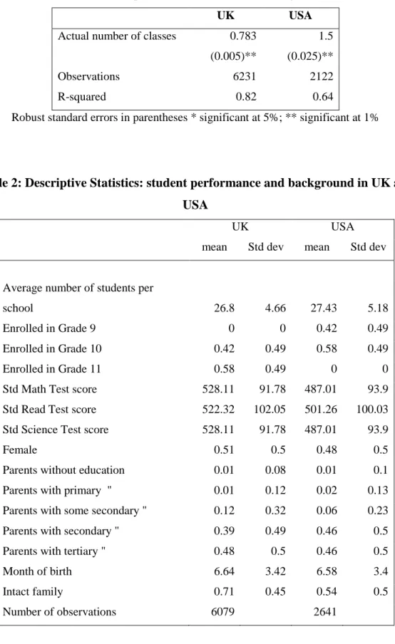
which information is collected. Table 1 presents the coefficients of this regression without the constant for the UK and the USA. The results show a high correlation between the expected number of classes and the actual one. The coefficient for the UK is significant at the 1% level and close to 1; whilst the coefficient for the USA, also well determined, is somewhat higher. The R2 shows that the regression explains 82 percent of total variation in the UK and 64 percent in USA. Therefore, our instruments, although probably measured with error should be good instruments for class size.
3. Descriptive Statistics
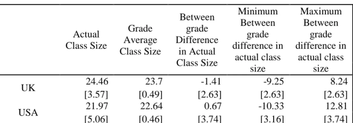
Table 2 presents descriptive statistics of the selected dataset. In every school an average of 27 students are tested for both United States and United Kingdom. The distribution of students between two adjacent grades is identical: in United Kingdom 42 percent of students tested are enrolled in grade 10, whilst 58 percent in grade 11; in United States students the same holds one grade behind. These values show that there is a representative sample of students in two adjacent grades in both the USA and UK sample. The scores are normalized to have a mean and standard deviation of 500 and 100 respectively.
Looking at the performance test English students perform better than American ones in the three subjects tested, math, science and reading. However, the difference could be due to the fact that English students are enrolled one grade ahead than Americans. In addition, when considering background characteristics, in the sample of English students there are more sons of parents with some secondary education and tertiary than in the American sample; whilst there are more children whose parents have completed secondary education in the sample of Americans. The fraction of children living in an intact family is significantly higher in the United Kingdom (71 percent) than in United States (54 percent).
In Table 3 descriptive statistics on class size are presented for the sample of students tested in mathematics. The average actual class size is lower in the United States (22 students) than in the United Kingdom (24.5). The averages at the country level of the grade average class size in the schools (second column) are similar to the values in the
12
first column. The correlation between the two values shows that the grade average class size is a good instrument for actual class size. Column 3 reports the between grade differences in average class size computed at the school level. The values displayed show that there are not significant differences in average class size between grade 9 and 10 for United States and between grade 10 and 11 for United Kingdom. Thus, it seems that there are no institutional differences in the rules determining class size between two adjacent grades, which means that all the between grade difference is due to random fluctuations in the students population. The standard deviation of the between grade differences in class size is comparable to the variation in actual class size for both countries, although the first is slightly lower. Furthermore, columns 4 and 5 show the minimum and the maximum of the difference in the average class size between grades in a school for both countries, providing further information on the range of variation in class size.
4. Results
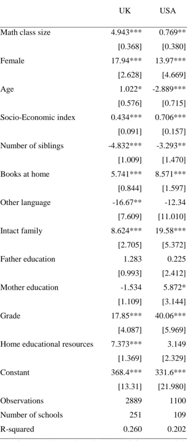
Estimates of class size effects based on the two different methods illustrated in Section 2 for the United Kingdom and the United States are presented in Table 4. The reported results control for grade level and the set of student and family background variables discussed in Section 2. Within each country, PISA conducted a stratified sampling design at the school and student level. Thus, we weight all the estimations by students’ sampling weights in order to obtain nationally representative coefficients. Moreover, the hierarchical structure of the data requires the addition of an error component at the school level in order to allow within school correlation. The clustering-robust linear regression delivers consistent estimation of the standard errors as it requires that observations are independent only within schools.
Table 4 reports the coefficient of class size from a standard least-square estimation as in equation (1). The results take into account between school selection by controlling for school fixed effects. Both estimates, for the UK and Unites States, have a positive significant sign, suggesting that students in larger classes perform better than students in smaller classes. The effect is about 7 times higher in UK than the US. So the results
13
imply that in the UK an increase in class size of 1 (relative to a mean of 24.6) increases the test score by just under 1% or just over one standard deviation.
Although we are controlling for between school differences, the naïve estimates support the counterintuitive result that students fare better in larger classes. However, the coefficients cannot be interpreted as causal effects, because this strategy does not eliminate the bias induced by within school sorting.
Table 5 presents the results from the IV strategy presented in Section 2. Columns 1 and 3 reports the coefficients of the instrument on actual class size controlling for school fixed effects, grade level, and the whole set of student and family background characteristics included in the outcome regression. Grade average class size is highly correlated with actual class size and statistically significant, indicating that average class size is not a weak instrument. The coefficients reported in the second and fourth columns of Table 5 present the estimates of the effect of class size on students’ math score respectively for the UK and USA. The estimated coefficient is positive and significant in the UK and positive and not significant in the USA. Using the IV method we do not detect a statistically significant effect of class size on student achievement for schools in United States. This result is consistent with the results found by Hoxby (2000), who identifies causal class-size effects by using class-size variations caused by natural fluctuations in cohort sizes. Also, it is consistent with the conclusions drawn by Hanushek (1999, 2003), who counts a high number of studies in the United States that report estimates of class size that are not statistically significant.
The F statistic reported at the end of the table is the test for the joint significance of the instruments (one in this case) in the first stage. The rule of thumb is that a value less than 10 indicates weak instruments. The Kleinbergen-Paap χ2 test is a test for under-identification.
However, we still obtain a counter-intuitive statistically significant positive effect for schools in UK. If we consider the literature on the effects of class size on students’ achievement in the UK, the “wrong sign” is found also by Darlington and Cullen (1982) and Dolton and Vignoles (1999). The reason relies on the compensatory resources arrangements applied by the UK system of educational funding. It includes a compensatory measure that allocates resources to local educational authorities on the basis of pupil numbers weighted by factors that reflect their social needs. The Ofsted
14
Report (1985) finds that Local Educational Authorities in inner-urban schools in the UK tend to have lower pupils-teacher ratio than other schools. Therefore, as Goldstein and Blatchford (1998) argue, the relationship between class size and pupil attainment is affected by schools placing lower attaining children in smaller classes and better teachers in larger classes. An alternative explanation looks to how parents decide on a portfolio of investments in their children. Parents can invest in their children in a number of ways, by investing in good quality schooling, investing in their health, by spending a lot of time with them or other means. So it is possible that higher levels of one investment “crowd out” other investments. In simple terms, at the margin a good school becomes an alternative to good parenting. In both the US and the UK most students attend a local public school, local being defined by school district and local educational authority (LEA) respectively. So, apart from migration, choice of school is typically exogenous. Hence one expects the causality to go from quality of school to quality of parenting7. So it is possible, depending on how one controls for parenting (if at all) to find a negative effect of education quality on attainment. Datar and Mason (2008) find some evidence of this crowding out in a sample of kindergarten and 1st grade children whereby increases in class size are associated with an increase in parent financed activities. It is also possible that students themselves respond to the perceived quality of school although it is unclear whether, for example, knowing that one has a good teacher will induce one to work more or less intensively.
Table 6 presents the results obtained by applying the alternative Lewbel approach to correct for within school sorting. Because identification requires heteroscedasticity (equation (5)), we next test for the presence of heteroscedasticity. The modified Wald test for heteroscedasticity shows that heteroscedasticity is strong in the first-stage regression models both in the UK and USA. Then, we multiplied the residuals obtained from the first stage regressions with two exogenous variables (female and age) centered at their sample mean. This gives us two instruments that we use as a means of identification for the IV estimates presented in Table 6 in the first and third columns. Moreover, these instruments can be combined with the instrument defined in the identification strategy outlined in Section 2. The second and the fourth columns of Table 6 report the results of the estimates using both the average class at the grade level
7 Note that this potential trade-off is independent of the fact that more affluent parents can be expected to
15
and the products between the first stage residuals and the two exogenous variables as instruments for the class size. The results are qualitatively unchanged, although the coefficients of class size are higher than those obtained with the IV strategy. The combination of instruments gives results that are closer to the estimates obtained in Table 5. When considering the size of class size effects in the educational production function, the effect ranges between 6 and 14 percent in the UK, whilst the estimates are not statistically significantly in the USA.
5. Conclusions
This paper finds, using large representative samples of high school students in the United States and the United Kingdom, that students do better on mathematics tests if the classes are larger. In the OLS models the class size coefficients are statistically significant. Controlling for the endogeneity of class size using two different methods individually and in conjunction leads to larger coefficients but they are not well determined in the case of the United States.
This finding may appear to be counter-intuitive but it is by no means unusual. Some authors (notably Dobbelstein et al (2002)) have explained this pattern by pointing to social psychological explanations whereby a student does better when in a class with many students similar to oneself. The larger the class is the more students there are who are similar, ceteris paribus. While peer effects such as this are possible, controlling for endogeneity of the class composition is essential. Levin (2001) uses a “Maimonides Rule” type approach to identifying class size effects using quantile regression applied to Dutch data. He also finds a positive slope with regard to class size which is attributed to peer effects.
A second possible explanation, discussed in the previous section, points to compensating behaviour by parents whereby parents choose a portfolio of investments in their children which may include their own time and efforts as well as school quality. Other things being equal then, high levels of school quality may point to low levels of parental inputs. The key factor then is the need to control for all investments in the child’s education which may be very data dependent.
16
A third possibility is that the teaching style used in a class depends on class size. Teachers facing a larger class may feel compelled to adopt a more didactic or more disciplined style. If so, then the question is whether such a method is effective. Clear evidence on the relative effectiveness of teaching styles appears to be rare. The study by Bennett (1976) argues that more formal teaching styles were more effective. Aitken et
al (1981) carefully analyses the effect of teaching styles using the same data and does
not find well determined effects. In neither case is there an explicit link to class size. Nonetheless the possibility of such a link may be worth considering in subsequent studies particularly if it is possible to design the data collection or indeed conduct an experiment.
The implicit assumption that smaller classes are better in general is based on a theory that a teacher allocates more time per student when there are fewer students or they may find it easier to exercise discipline. This, in turn, is assumed to lead to higher achievement by students. However this is only a theory in the sense that invariably neither discipline nor time-per-student is observed in the data and their effects on achievement can only be conjectured. Teachers may simply work less hard. The latter possibility may seem an extreme assumption but in the absence of good data on the processes occurring in classrooms it seems prudent to keep a very open mind on what one expects to find.
An across-the-board policy of reducing class size will in general be an expensive investment in education though there may be particular circumstances or populations (such as students in need of remedial classes or immigrant students) where it can be demonstrated to be warranted. The evidence presented here suggests that aside from being expensive it is also counter-productive.
17
Table 1. Expected number of classes by grade
UK USA
Actual number of classes 0.783 1.5
(0.005)** (0.025)**
Observations 6231 2122
R-squared 0.82 0.64
Robust standard errors in parentheses * significant at 5%; ** significant at 1%
Table 2: Descriptive Statistics: student performance and background in UK and USA
UK USA
mean Std dev mean Std dev
Average number of students per
school 26.8 4.66 27.43 5.18
Enrolled in Grade 9 0 0 0.42 0.49
Enrolled in Grade 10 0.42 0.49 0.58 0.49
Enrolled in Grade 11 0.58 0.49 0 0
Std Math Test score 528.11 91.78 487.01 93.9 Std Read Test score 522.32 102.05 501.26 100.03 Std Science Test score 528.11 91.78 487.01 93.9
Female 0.51 0.5 0.48 0.5
Parents without education 0.01 0.08 0.01 0.1 Parents with primary " 0.01 0.12 0.02 0.13 Parents with some secondary " 0.12 0.32 0.06 0.23 Parents with secondary " 0.39 0.49 0.46 0.5 Parents with tertiary " 0.48 0.5 0.46 0.5
Month of birth 6.64 3.42 6.58 3.4
Intact family 0.71 0.45 0.54 0.5
18
Table 3: Descriptive Statistics: Class size in the Math Sample
Actual Class Size Grade Average Class Size Between grade Difference in Actual Class Size Minimum Between grade difference in actual class size Maximum Between grade difference in actual class size UK 24.46 23.7 -1.41 -9.25 8.24 [3.57] [0.49] [2.63] [2.63] [2.63] USA 21.97 22.64 0.67 -10.33 12.81 [5.06] [0.46] [3.74] [3.16] [3.74]
19
Table 4. OLS Estimates in Maths score – UK&USA
UK USA
Math class size 4.943*** 0.769**
[0.368] [0.380] Female 17.94*** 13.97*** [2.628] [4.669] Age 1.022* -2.889*** [0.576] [0.715] Socio-Economic index 0.434*** 0.706*** [0.091] [0.157] Number of siblings -4.832*** -3.293** [1.009] [1.470] Books at home 5.741*** 8.571*** [0.844] [1.597] Other language -16.67** -12.34 [7.609] [11.010] Intact family 8.624*** 19.58*** [2.705] [5.372] Father education 1.283 0.225 [0.993] [2.412] Mother education -1.534 5.872* [1.109] [3.144] Grade 17.85*** 40.06*** [4.087] [5.969]
Home educational resources 7.373*** 3.149
[1.369] [2.329] Constant 368.4*** 331.6*** [13.31] [21.980] Observations 2889 1100 Number of schools 251 109 R-squared 0.260 0.202
20
Table 5. IV Estimates for Mathematics score – UK & USA
UK USA
First stage IV First stage IV
Average math class 0.161 0.815
[0.048]** [0.143]**
Math class size 6.015** 1.594
[3.041] [2.020] Female -0.547 22.29*** -0.394 13.88*** [0.303] [3.924] [0.406] [4.700] Age 0.054 0.692 -0.034 -3.088*** [0.069] [0.828] [0.070] [0.806] Socio-Economic index 0.032 0.383** 0.009 0.627*** [0.013]* [0.169] [0.016] [0.166] Number of siblings -0.084 -4.509*** -0.022 -4.021*** [0.133] [1.207] [0.138] [1.552] Books at home 0.368 4.928*** 0.06 9.878*** [0.111]** [1.465] [0.152] [1.758] Other language -0.101 -23.54*** 1.988 -16.46 [0.725] [9.006] [1.071] [15.400] Intact family 0.809 8.825** -0.121 18.88*** [0.355]* [3.836] [0.494] [5.132] Father education -0.138 3.630*** -0.081 1.801 [0.128] [1.332] [0.265] [2.461] Mother education 0.139 0.621 0.293 7.493** [0.133] [1.538] [0.294] [3.348] Grade -1.63 21.48*** 0.529 40.39*** [0.551]** [8.288] [0.497] [6.573]
Home educational resources 0.371 6.366*** -0.194 2.715
[0.172]* [2.221] [0.239] [2.709] Observations 2889 2888 1100 1099 Number of schools 250 108 Root MSE 5.44 60.65 6.19 64.31 F statistic F(1, 249)=11.11 F(1,107)=50.16 P value 0.001 0.000
Kleibergen-Paap Wald statistic χ2(1)=11.20 χ2(1)=51.14
P value 0.001 0.000 0.440
21
Table 6. “Lewbel” estimates in Mathematics scores – UK & USA
UK USA
Lewbel Lewbel and IV Lewbel Lewbel and IV
Math class size 14.59* 8.341** 7.145 2.107
[7.520] [2.856] [10.020] [1.896] Female 27.05*** 23.58*** 16.30** 14.10** [7.670] [4.740] [7.408] [5.513] Age 0.216 0.563 -2.816* -3.063*** [1.372] [0.806] [1.490] [0.839] Socio-Economic index 0.119 0.312** 0.562* 0.621*** [0.383] [0.156] [0.315] [0.183] Number of siblings -3.719** -4.295*** -3.86 -4.006** [1.816] [1.408] [2.390] [1.710] Books at home 1.816 4.084** 9.706*** 9.862*** [2.939] [1.870] [3.039] [1.558] Other language -22.810 -23.34** -27.6 -17.49 [15.220] [11.120] [39.860] [14.120] Intact family 2.042 6.985 19.15** 18.90*** [7.678] [4.481] [9.765] [4.749] Father education 3.017 5.457** 0.35 1.667 [4.148] [2.395] [6.025] [3.052] Mother education 1.675 0.907 7.986* 7.538** [2.339] [1.628] [4.571] [3.747] Grade 10/Grade 11 2.397 3.296* 35.16* 39.91*** [2.573] [1.702] [19.120] [6.934]
Home educational resources 41.27* 26.84** 4.083 2.842
[21.170] [10.620] [5.277] [2.792] Observations 2889 2889 1100 1100 Number of schools 250 250 108 108 Root MSE 80.11 63.15 74.9 64.58 F statistic F(2, 249)=2.91 F(3,249)=4.62 F(2, 107)=1.72 F(3, 107)=18.32 “ “ p value 0.056 0.003 0.185 0.000
Kleibergen-Paap Wald statistic χ2 (2)=5.87 χ2 (3)=13.98 χ2 (2,107)=3.50 χ2(3,107)=56.13
“ “ p value 0.053 0.003 0.173 0.000
22
References
Aitken, M, D.Anderson and J. Hinde (1981) Statistical modelling of data on teaching styles, Journal of the Royal Statistical Society A, 144(4), 419-461
Akerhielm, K. (1995) Does class size matter? Economics of Education Review, 14(3), 229-241
Angrist, J. and V. Lavy (1999) Using Maimonides rule to estimate the effect of class size on scholastic achievement Quarterly Journal of Economics, 114(2), 533-575
Barnett, N. (1976) Teaching style and pupil progress Open Books, London
Belfield, C.R. and I. Rashad Kelly (2010) The benefits of breastfeeding across the early childhood years. NBER working paper 16496
Burtless, G. (editor) (1996) Does money matter? The effect of school resources on
student achievement and adult success, Brookings Institution, Washington, D.C.
Case, A. and A. Deaton (1999) School inputs and educational outcomes in South Africa
Quarterly Journal of Economics, 114(3), 1047-1084
Darlington, J.K. and B.D. Cullen (1982), Pilot Study of School Examination
Performance and Associated Factors, DES: London
Datar, A. and B. Mason (2008) Do reductions in class size “crowd out” parental investment in Education?, Economics of Education Review, 27, 712-713
Dearden L., J. Ferri and C. Meghir (2002) The effect of school quality on educational attainment and wages, Review of Economics and Statistics, 84(1), 1-20
Dolton P. and A. Vignoles (1999) The Impact of School Quality on Labour Market Success in the UK, Discussion Paper No. 98-03, University of Newcastle
Dobbelstein, S., J. Levin and H. Oosterbeek (2002) The causal effect of class size on scholastic achievement: distinguishing the pure class size effect from the effect of changes in class composition, Oxford Bulletin of Economics and Statistics, 64, 17-38
Dustmann C., N. Rajah, and A. van Soest (2003) Class size, education and wages,
Economic Journal, 113, 1-53
Feinstein, L and J. Symons (1999) Attainment in secondary school, Oxford Economic
23
Goldstein, H. and P. Blatchford (1998), Class Size and Educational Achievement: A Review of Methodology with Particular Reference to Study Design, British Educational
Research Journal, 24(3), 255-267
Hansen, L.P. (1982) Large sample properties of generalized method of moments estimators Econometrica, 50, 1029-1054
Hanushek, E.A. (1999) “The evidence on class size” in Earning and Learning: how
schools matter (editors Susan E. Mayer and Paul E. Peterson) Brookings Institution
Press, Washington D.C. and Russell Sage Foundation, New York
Hanushek, E.A. (1994) Money might matter somewhere: a response to Hedges, Laine and Greenwald, Educational Researcher, 23(4), 5-8
Hanushek, E.A. (2003) The failure of input-based schooling policies, Economic
Journal, 113 (485), 64-98
Hedges, L.V., R.D. Laine and R. Greenwald (1994) Does money matter? A meta-analysis of studies of the effects of differential school inputs on student outcomes
Educational Researcher, 23(3), 5-14
Hedges, L.V., R.D. Laine and R. Greenwald (1994) Money might matter somewhere: a reply to Hanushek, Educational Researcher, 23(4), 9-10
Hoxby C. (2000) The effect of class size on student achievement: new evidence from population variation Quarterly Journal of Economics, 115(4), 1239-1285
Klein R. and F. Vella (2003) Identification and estimation of the triangular Simultaneous Equation model in absence of exclusion restrictions through the presence of heteroskedasticity, unpublished manuscript
Krueger A. (1999) Experimental Estimates of Education Production Functions”
Quarterly Journal of Economics, 114(2), 497-532
Krueger A. (2003) Economic considerations and class size, Economic Journal, 113, 34-63
Levin, J. (2001) For whom the reductions count: a quantile regression analysis of class size and peer effects on scholastic achievement Empirical Economics, 26, 221-246
24
Lewbel A. (2010) “Using heteroskedasticity to identify and estimate mismeasured and endogenous regressor models”, Economics Department, Boston College mimeo
OFSTED (1995), Class Size and the Quality of Education, HMSO, London
Kelly Rashad, I. and S. Markowitz (2009/2010) Incentives in obesity and health insurance Inquiry 46(4), 418-432
Rigobon R. (2002) “Identification through Heteroskedasticity” Review of Economic and
Statistics, 85(4), 777-792
Sabia, J.J. (2007) “The effect of body weight on adolescent academic performance”
Southern Economic Journal, 73, 871-900
Woessmann L. and M. West (2006) “Class-size effects in school systems around the world: Evidence from between-grade variation in TIMSS” European Economic Review, 50 , 695-736