NBER WORKING PAPER SERIES
OPTIMAL INCOME TRANSFERS Louis Kaplow
Working Paper 12284
http://www.nber.org/papers/w12284
NATIONAL BUREAU OF ECONOMIC RESEARCH 1050 Massachusetts Avenue
Cambridge, MA 02138 May 2006
Harvard University and National Bureau of Economic Research. I am grateful to workshop participants and the referees for comments, Mary Bear, Ivan Chen, Eun Young Choi, Vicki Chou, Zachary Gubler, Jeffrey Harris, Jonathan Lin, Ned Locke, Kathleen Saunders, and Kevin Terrazas for research assistance, and the John M. Olin Center for Law, Economics, and Business at Harvard University for financial support. The current paper traces its origins to a book project, Kaplow (forthcoming). The views expressed herein are those of the author(s) and do not necessarily reflect the views of the National Bureau of Economic Research.
©2006 by Louis Kaplow. All rights reserved. Short sections of text, not to exceed two paragraphs, may be quoted without explicit permission provided that full credit, including © notice, is given to the source.
Optimal Income Transfers Louis Kaplow
NBER Working Paper No. 12284 May 2006
JEL No. H21, H53, I38
ABSTRACT
A substantial literature addresses the design of transfer programs and policies, including the negative income tax, other means-tested transfers, the earned income tax credit, categorical assistance, and work inducements. This work is largely independent of that on the optimal nonlinear income tax, yet formulations of such a tax necessarily address how low-income individuals should be treated. This paper draws on the optimal income taxation literature to illuminate the analysis of transfer programs, including the level and shape of marginal tax rates (including phase-outs), the structure of categorical assistance, and the role of work inducements in an optimal income transfer scheme. Louis Kaplow Harvard University Hauser Hall 322 Cambridge, MA 02138 and NBER moverholt@law.harvard.edu
1See, for example, Atkinson (1995), Garfinkel (1982), Green (1967), Meyer and
Holtz-Eakin (2001), and Moffitt (2002, 2003).
2See, for example, Mirrlees (1971), Atkinson and Stiglitz (1980), Stiglitz (1987), and
Tuomala (1990). 1. Introduction
Income transfers to low-income individuals have been the subject of a great deal of scholarly attention, and for good reasons. Many programs target the poor and near-poor, and these systems have been a continuing subject of controversy and reform. Low-income
individuals are often believed to have certain traits – disabilities, age, or dependents – that render work difficult or inappropriate, thereby requiring income support. Moreover, under most
standard social welfare functions and plausible individual utility functions, the marginal social welfare weight per dollar is substantially greater at the bottom end of the income distribution, so the design of income transfer programs is of great social consequence.
Most existing literature focuses on specific transfer schemes or particular characteristics thereof. Over the years, subjects receiving the most attention include the negative income tax and related systems, means-testing of transfer programs, earnings subsidies such as the earned income tax credit (EITC) in the United States tax system, categorical assistance, and other work inducements.1 Analyses often isolate one or more features, such as program cost, work
incentives, or effectiveness in targeting the needy. This work does not, however, typically
provide a comprehensive assessment or attempt to determine what overall plan would be optimal. There also exists an important body of work on optimal nonlinear income taxation.2 This
literature offers both analysis – which, although technically demanding, does yield first-order conditions that may be interpreted intuitively – and simulations. Of particular relevance for present purposes, the “income tax” examined in this literature does not correspond simply to a typical personal income tax schedule but rather encompasses all taxes and transfers. The schemes examined feature a grant, implicitly received by everyone, combined with a tax that depends on the level of income.
3As will be explored in section 3, one can readily extend the analysis to allow different
schedules for different types of individuals or family units.
4A complication is that some transfer programs have a so-called cliff or notch effect, such
that when income reaches a particular point, certain benefits are lost altogether; that is, some Ti(y) may be discontinuous, so T(y) may not be defined at such points. (There also may be kinks in the tax schedule, but these are less troublesome for most analysis.) Such complications will generally be ignored here.
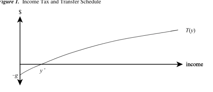
Figure 1. Income Tax and Transfer Schedule
In Figure 1, the schedule T(y), showing taxes as a function of income, is a single,
integrated tax and transfer scheme. Individuals who earn no income receive the grant g = T(0), those earning income y° are at the breakeven point at which the taxes they owe just equal the grant, and those earning more than y° pay positive net taxes.3 However, one can just as easily
interpret Figure 1 as depicting an income tax that exempts income below y° combined with a separate transfer scheme that provides g, which is fully phased out when income reaches y°. (There are additional possibilities: T(y) could be viewed as a standard income tax with an exemption less than y°, including one with no exemption, combined with a transfer scheme that provides g, which is not fully phased out until income reaches a level above y°.) Furthermore, in examining actual systems of transfer programs, one can interpret g as the sum of all forms of assistance available to those earning no income, and the marginal tax rate T (y) can be taken as the sum of the explicit marginal tax rates of the income tax and other pertinent taxes and the phase-out rates of various transfer programs. In other words, each tax and each transfer program can be represented by its own schedule Ti(y), and we can let T(y) = Ti(y).4
Suppose that one has determined an optimal income tax schedule for a given society; perhaps it is that depicted in Figure 1. Then, a fortiori, one has determined the optimal system of income transfers, for that is indicated by the lower end of the very same income tax schedule. Likewise, one has determined how best to reform an existing system: If one subtracts the aggregate existing schedule from the optimal schedule, the difference indicates what reform of taxes and transfers would move the system to the optimum.
This approach to optimal income transfers differs substantially from that in most of the pertinent literature. Existing work, as noted, tends to focus on particular transfer programs or transfer programs as a whole. Changes in such programs, however, are not generally revenue-neutral and are almost never distribution-revenue-neutral, so unless one also considers effects on the rest of the population and aggregates them with a social welfare function, it is difficult to know what changes would be optimal. Even clear indicators may be misleading because they are partial: A program may reduce outlays or labor supply distortion, but at the expense of redistribution; a reform may improve work incentives, but since the optimum involves some degree of work disincentive, one cannot know whether the move is in the right direction. Moreover, it is familiar from research on optimal income taxation that an important effect of changing the marginal income tax rate at any given level of income – and particularly at low levels of income – is the inframarginal impact on those with higher incomes. Accordingly, it is difficult to illuminate questions about optimal income transfers by confining attention to explicit transfer programs at the lower end of the income distribution.
An additional limitation is that much work focuses on very specific programs, whether existing, proposed, or hypothetical. As just one component Ti(y) of the overall schedule T(y), there is no sense in which any particular program can be assessed or optimized without regard to the rest of the system. To be sure, if all other taxes and transfers are accounted for and taken as given, one can speak meaningfully of optimal reform of a single component, but if the
component is restricted in various ways – for example, if the reform cannot change the grant g or if any adjustment to marginal tax rates is limited to lower-income individuals and must have a prescribed shape (say, that of the EITC) – the results may obscure the best paths for reform. (If aggregate marginal tax rates, including outs, were too high in both the in and phase-out ranges of the EITC, making the EITC more or less generous might be desirable if no other change is possible, but such a reform would be largely orthogonal to the true problem.)
Furthermore, it is necessary to be consistent (and plausible) regarding what policy
instruments are assumed to be feasible. For example, if a form of work requirement necessitates that hours and thus implicitly wage rates be observable, such information could be used to implement a tax-transfer scheme that was less distortionary than (and qualitatively different from) typical work inducement proposals. But if such a scheme could readily be circumvented due to the manipulability of reported hours, which is commonly supposed, then the more conventional work inducement may be impractical as well.
The purpose of this article is to analyze optimal income transfers as part of the broader optimal income taxation problem. This approach is initially advanced in Diamond’s (1968) review of Green’s (1967) book on the negative income tax. Diamond focused on how to choose transfer schedules optimally, foreshadowing important elements of the literature on optimal income taxation that appeared shortly thereafter. Furthermore, characterizing optimal income transfers was one of the motivations offered by Mirrlees (1971) for his exploration of the optimal nonlinear income tax, and he remarked on the inability to address transfers without regard to the rest of the income tax schedule. In a sense, the present article aims to pick up where Diamond
5A subset of the literature on income transfers seeks to examine optimal schemes. See,
for example, Liebman (2001), the writing on categorical assistance surveyed in subsection 3.3, and some of the literature on work inducements discussed in subsection 4.4. However, little research takes advantage of the general, flexible, and encompassing framework offered by the work on optimal nonlinear income taxation, and accordingly it is not able to generate many of the insights produced here.
(1968) and Mirrlees (1971) left off, taking advantage of insights in the subsequent literature.5
Section 2 provides the most direct application of results on optimal nonlinear income taxation. Initially, the standard first-order condition for that problem is presented in an intuitive form (which has appeared in some of the writings since Mirrlees (1971)) and interpreted with special emphasis on the lower end of the income distribution. Additionally, results from simulations are noted. Both the analysis and the simulation results support – very roughly – fairly high marginal rates at the bottom, although lower than existing aggregate marginal rates that can approach or even exceed one hundred percent. Furthermore, in the low to moderate income range, the level of optimal marginal rates is fairly flat or gradually declining, which stands in sharp contrast to the very large drops in marginal rates (notably, at the end of phase-out ranges) in existing systems and under many proposals. It is suggested that existing thought and practice reflects misplaced emphasis on the idea that transfers need to be phased out quickly and, once they are, that marginal tax rates should be fairly low on moderate-income individuals. These conclusions are applied to existing discourse about extremely high aggregate marginal tax rates, the design of the EITC, and other matters.
Section 3 examines categorical assistance, such as special programs targeted at the disabled, elderly, or families with young children. Analytically, the approach involves a modest modification to the optimal income tax model already set forth, which can then be interpreted to illuminate the optimal design of categorical assistance. Most discussion focuses on the realistic setting in which categorization is imperfect; for example, some classified as able may be disabled and some deemed to be disabled may nevertheless have high earning ability. It turns out that the optimal tax and transfer schemes for such two-category systems are qualitatively different from each other. It is not simply the case that the more able group receives less generous assistance. It also seems plausible that the schedule of marginal tax rates is distinctive, and in a manner that deviates from common thinking and practice. Specifically, it may be optimal to apply higher marginal tax rates (phase-outs) to the group receiving lower assistance, even though there are only modest benefits to “phase out,” while applying lower rates to the group receiving more generous assistance. Once again, understandings based on the supposed need to phase out program benefits can be misleading.
Section 4 analyzes schemes that embody work inducements of various sorts. As will be explained, many work incentive plans do not literally require work but instead adjust benefits in light of earnings or work effort. In other words, individuals who are classified as able but do not meet target levels of work effort have their benefits reduced or eliminated. It turns out that the optimal design of earnings-based work inducements is implicit in the analysis of section 3.
6A range of additional topics – including whether assistance should be provided in cash or
in kind, concerns involving two-earner families, labor market interventions such as a minimum wage or subsidies to the development of human capital, effects of transfers on wage levels, and insurance such as for temporary unemployment – are beyond the scope of this article, although the framework advanced here should prove useful for exploring them as well.
7Although the formulation in the text is standard in the literature, one might question the
extent to which individuals, especially low-income individuals who tend to be less sophisticated and face multiple marginal rates from a variety of complex programs, choose labor supply as the theory of the perfectly informed rational maximizer would predict. Low-income individuals may be more aware of average than marginal rates, but may approximately learn marginal rates over time as they vary their work effort or obtain information from others similarly situated. In the absence of empirical evidence on the structure of individuals’ misperceptions, it is not apparent Having already determined the optimal scheme for individuals classified as able, the analysis is essentially complete. Moreover, the optimal scheme does not have the characteristics of standard work incentive programs. A different case arises if not only earnings but also the amount of work effort can be observed. If there is perfect observability of effort, schemes better than and qualitatively different from standard work requirements become feasible. In the more realistic case of imperfect observability, features of the preceding analysis become applicable, with the implication that important features of various work requirement plans are not optimal.6 Finally,
this section explores the important possibility – which may underlie welfare reforms in recent decades – that there are various sorts of externalities to work of low-income individuals and then considers how such externalities would affect the analysis.
2. Optimal Income Taxation and Optimal Income Transfers 2.1. Framework
The standard optimal nonlinear income tax model has the following basic elements. An individual’s utility is given by u(c,l), where c is consumption and l denotes labor effort. An individual’s consumption (equivalent to disposable income) is given by
( )
1
c wl T wl
=
−
( ),
where w is the individual’s exogenously given wage rate. Individuals’ pre-tax earnings are the product of their wage and effort level, that is, y = wl. The motivation for redistributive taxation is that individuals differ in their wages, that is, their earning abilities. The distribution of abilities is given by F(w), with density f(w), the population being normalized to have a total mass of one. Furthermore, it is supposed that the government cannot directly observe individuals’ abilities – if it could, any distributive objective to be achieved with nondistortionary individualized lump-sum taxes – and thus must rely on distortionary income taxation.
Individuals choose the level of labor effort l that maximizes u(c,l) subject to their budget constraint (1).7 The government’s problem is taken to be the choice of a tax-transfer schedule
how this potentially important complication is best analyzed, but absent reasons to believe that there are large, systematic errors, one suspects that the rough guidance provided by standard analysis remains illuminating.
8In addition to Diamond (1998 (expression (10) on page 86), see Atkinson and Stiglitz
(1980) (expression (13-54) on page 417), Stiglitz (1987) (expression (25) on page 1007 and the expression in note 17 on page 1008), Dahan and Strawczynski (2000) (expression (2) on page 682), and Auerbach and Hines (2002) (expressions (4.12) and (4.15) on pages 1381-82). Expression (4) is also similar to the two formulations in Saez (2001, p. 215); an important difference involves the attention he devotes to translating the results from ones in terms of the distribution of abilities (which is unobservable) to ones in terms of the distribution of income (taking into account that the tax rules and other parameters will determine the relationship between the ability distribution and the resulting income distribution).
T(wl) to maximize social welfare,
(
)
(
)
( )
2
W u c w l w
( ), ( )
f w dw
( )
,
where c and l are each expressed as functions of w to refer to the level of consumption achieved and labor effort chosen by an individual of type (ability) w. This social maximization is subject to a revenue constraint and to a set of constraints regarding individuals’ behavior. The former is
( )
3
T wl w f w dw R
( ( )) ( )
=
,
where R is an exogenously given revenue requirement. Here, revenue is to be interpreted as expenditures on public goods that should be understood as implicit in individuals’ utility
functions; because these expenditures are taken to be fixed, they need not be modeled explicitly. Regarding the latter set of constraints, individuals are assumed to respond to the given tax
schedule optimally, that is, by choosing labor effort to maximize their own utility, taking the tax schedule as given.
2.2. Analysis
Much of the analysis can be summarized in a first-order condition for the optimal marginal tax rate at any income level y*, where w* and l* correspond to the ability level and degree of labor effort supplied by the type of individual who would just earn y*. Following the presentation in Diamond (1998) – which makes the simplifying assumptions that utility is separable between consumption and labor effort and that marginal utility uc is constant – the condition can be expressed as8
9This sort of perturbation is discussed in Diamond (1968), and he offers the conjecture
that optimal rates at the bottom are high, for reasons that overlap with those offered in the text to follow. See also Saez (2001).
10There are a variety of reservations to any such interpretation. One set concerns the fact
that all values are endogenous, so differing presumed values of one component affect the values of others at the optimum. Another is that the problem is not necessarily well behaved. In particular, in regions of falling marginal tax rates or fixed costs of labor market participation, small changes in the tax schedule may lead individuals to “jump” from one level of income to another, in which case a different condition governs their behavior and there would be gaps in the resulting income distribution. In addition, simplifications such as the assumption that uc is constant, which rules out income effects, have been employed. Such complexities are largely ignored for present purposes, but they may prove important, especially in designing simulations. See also the discussion of the participation decision in subsection 4.4.
( ) ( * *) ( * *) ( *) * * ( *) ( ( )) ( ) ( *) , * 4 1 1 1 1 ′ − ′ = − − ′ − ∞ T w l T w l F w w f w W u w u f w dw F w c w
ξ
λ
where primes indicate derivatives with respect to a function’s only argument, is the shadow price of government revenue, and * = 1/(1+l*ull/ul) – which, when utility is quasi-linear as assumed here, equals /(1+ ), where is the elasticity of labor supply. Note that this formulation (like those in recent literature) includes 1 F(w*) in both the numerator and the denominator on the right side. The motivation is that, in the first term, (1 F(w*))/f(w*) is purely a property of the distribution of w, and, in the second term, because the numerator is an integral from w* to , the term as a whole gives an average value for the expression in brackets in the integrand. Both aspects facilitate interpretation, as will be seen in the discussion to follow.
To aid in understanding expression (4), it is helpful to have in mind the simple
perturbation of the income tax schedule that underlies this first-order condition.9 If one begins
with some tax schedule T(wl), assumed to be optimal, it must be that no slight adjustment to the schedule will change the level of social welfare. Consider an adjustment that slightly raises the marginal tax rate at some income level, y* (say, in a small interval from y* to y*+ ), leaving all other marginal tax rates unchanged. There are two effects of such a change. First, individuals at that income level face a higher marginal rate, which will distort their labor effort, a cost. Second, all individuals above income level y* will pay more tax, but these individuals face no marginal distortion. That is, the higher marginal rate at y* is inframarginal for them. Since those thus giving up income are an above-average slice of the population (it is the part of the population with income above y*), there tends to be a redistributive gain.
Expression (4) can readily be interpreted in terms of this perturbation.10 Begin with the
first term. Revenue is collected from all individuals with incomes above y*, which is to say all ability types above w*; hence the 1 F(w*) in the numerator. One distorts only the behavior of the marginal type, which explains the f(w*) in the denominator. The larger is the fraction of the
11Another natural way to think of the experiment of raising the marginal rate T(w*l*) is
to suppose further that the additional revenue will be used to increase the uniform grant. The marginal social value of increasing the grant will, at the optimum, necessarily equal the shadow price of government revenue. Hence, the formulation in the text in which the rebate is not carried through but is given a shadow value is formally equivalent to what would obtain if one literally adhered to the revenue constraint by increasing the grant until the budget balanced. (This relationship of course is standard for constrained optimization that employs shadow prices.)
12Additionally, if one relaxed the assumption that u
c is constant, the resulting income effect would induce greater labor supply, which further increases revenue.
13Empirical evidence on the elasticity of taxable income tends to find higher elasticities
among higher-income individuals, apparently due to differences in tax avoidance opportunities. See Alm and Wallace (2000), Auten and Carroll (1999), Gruber and Saez (2002), and Moffitt and Wilhelm (2000). By contrast, Juhn, Murphy, and Topel (1991) find that uncompensated labor supply elasticities for men fall with income. It is suggested, however, that the broader concept of elasticity of taxable income is more relevant to welfare analysis because all margins of behavioral response to changes in tax rates involve the same marginal distortion. See Feldstein population paying more tax and the smaller is the group being distorted – or put more succinctly, the greater is the ratio of the former to the latter – the higher is the optimal tax rate. The
denominator also contains weights of *, indicating the extent of the distortion, and w*, indicating how much production (and thus tax revenue) is lost per unit of reduction in labor effort.
The second term applies a relative social weighting to the revenue that is collected from inframarginal individuals; it is an average weight for the portion 1 F(w*) that pays more tax. Regarding the numerator, the term in parentheses is the difference between the marginal dollar that is raised and the dollar equivalent of the loss in welfare that occurs on account of individuals above w* paying more tax: uc is the marginal utility of income to such individuals, W indicates the impact of this change in utility on social welfare, and division by , the shadow price on the revenue constraint, converts this welfare measure into dollars.11
We now consider what expression (4) reveals about optimal marginal rates at the lower end of the income distribution. It appears that fairly high rates may be optimal. Focusing on the first term on the right, we can see that three factors contribute to this result. First, the numerator, 1 F(w*), is large: Raising marginal rates on very low incomes raises substantial revenue
(allowing for a higher g) because most of the population has incomes higher than this level. Moreover, high rates at the bottom are inframarginal for this large group of individuals.12
Second, in the denominator, f(w*) is not very high, indicating that only a moderate portion of the population has their labor supply distorted by high marginal rates in this income range. Third, w* is low, so there is little lost productivity and thus revenue when such individuals reduce their labor supply. Fourth, although the elasticity component, *, is often taken to be constant, there is some evidence indicating that, if anything, the pertinent elasticity may be lower for low-income individuals, which would also contribute to a higher optimal marginal tax rate.13 There is,
(1999).
14At y* near zero, this offset would be complete if even the lowest-ability types worked.
This is the familiar “zero at the bottom” result of the optimal nonlinear income taxation
literature. See Brito and Oakland (1977), Seade (1977), and Ebert (1992). The usual argument for high marginal rates near the bottom of the income distribution is inapplicable when all earn above some minimum level because it is more efficient to reduce the grant g than to apply a positive marginal tax at the bottom. Put another way, raising the marginal rate from zero for the bottom person accomplishes no redistribution (everyone pays more tax and receives a
correspondingly higher grant) but does distort that individual’s labor supply. As the simulations to follow reveal, however, this force toward a zero rate at the bottom is not nearly complete if a significant number of low-ability individuals do not work at all, as is actually the case.
15The drop in Saez (2001), although atypical, is not that surprising in light of the
foregoing discussion of the first term of expression (4), specifically the ratio (1 F(w*))/w*f(w*).
however, a countervailing factor: The second term, reflecting the average welfare weight for individuals with abilities above w*, provides some offset to the argument for high marginal rates at the bottom.14 In this range, those inframarginal include some fairly low-income individuals,
and their welfare weight is relatively high. 2.3. Simulations
The conjecture that optimal marginal tax rates will be high at the bottom of the income distribution (and possibly higher than at middle or upper levels of income) is confirmed by simulations on the optimal nonlinear income tax. Mirrlees (1971) original simulations largely have marginal rates in the 20’s and 30’s at the low end of the income distribution although one case has rates in the high 50’s and as high as 60%. These low-end rates are the highest of the marginal rates in his simulations. Tuomala (1990) offers a wide range of simulations; with a utilitarian (rather than more concave) welfare function and his preferred substitution elasticity (table 6.1, cases 4-6), marginal rates at the tenth percentile of the income distribution are in the 40’s. Kanbur and Tuomala (1994) report results for differing degrees of inequality in the distribution of abilities and find rates at the bottom in the range 49% to 60%. Saez’s (2001) utilitarian base case has marginal rates at the bottom in the 70%-80% range. Additionally, Slemrod et al.’s (1994) simulations for the optimal two-bracket system find that the optimal lower bracket rate is approximately 60%, which is slightly higher than the optimal upper-bracket rate.
Whatever the absolute level of marginal rates in a particular simulation, it is typical for the optimal marginal rates just above the low end – running, say, from levels of income where welfare phase-outs ordinarily are complete to the median level of income – to be almost as high. In most instances, the falloff is only a few percentage points, with somewhat higher drops when the initial (bottom-end) rates are higher. Exceptions are Kanbur and Tuomala (1994), who report a rise in marginal rates in two of their three simulations and Saez (2001) who finds drops (from an initial level of 70-80%) of approximately 30% (with the lowest rate being reached at an income of about $75,000).15 The finding that marginal rates do not rapidly fall is to be expected
This explanation is suggested noting the similarity between Saez’s Figure 4, which graphs a similar relationship as a function of income, and his Figure 5, which graphs simulated optimal income tax schedules.
16See, for example, Dickert, Houser, and Scholz (1994), Keane and Moffitt (1991), and
Wilson and Cline (1994), and after welfare reform, Acs et al. (1998), Gokhale, Kotlikoff, and Sluchynsky (2002), Hepner and Reed (2004), and Shaviro (1999).
in light of the first-order condition. Although some factors favor falling rates, not all do and none is likely to favor precipitously declining rates for modest differences in income.
Finally, the optimum is typically characterized by a nontrivial fraction of individuals, those with the lowest abilities, choosing not to work at all. Mirrlees (1971) and Tuomala (1990) have approximately 5%-10% not working under the optimal scheme in most simulations,
although this percentage goes as high as 20%. This finding also is not surprising. Given that high marginal tax rates are optimal near the bottom and that a generous grant is provided,
individuals of very low ability are unlikely to find work worthwhile. (It is of course possible that some would have sufficiently low ability to render it optimal to abstain entirely from work even if the marginal rate at the very bottom were zero.) Furthermore, the productivity and therefore the revenue loss when such individuals do not work is small.
2.4. Implications
In the United States, there are multiple taxes and transfer programs relevant to many low-income individuals. Some transfer programs have very high phase-out rates, others more
gradual, and the tax system includes the EITC, which provides roughly a 40% marginal subsidy to low-income workers with two or more children but adds approximately a 20% tax in its phase-out range. Taken together, Giannarelli and Steuerle’s (1995) microsimulation suggests that the aggregate marginal tax rate (ignoring work expenses) is 75% or more for many low-income workers and above 100% for some. Examining programs as of 1998 (after welfare reform), Sammartino et al. (2002) find that a single parent with two dependents faces average marginal tax rates of about 60-70% when increasing earnings from half the poverty line to 125% thereof, of over 100% in moving to 150% of the poverty line, and of just over 30% beyond that point. Other studies reach similar conclusions.16
Such high aggregate marginal rates (inclusive of phase-outs) are generally criticized. As suggested above, optimal marginal rates at the low end are quite high, but simulations do not suggest that they should be as high as actually exists. Furthermore, once past the phase-outs of transfers (including the EITC), existing aggregate marginal rates seem to be below what is optimal. Likewise, many proposals over the years, including the negative income tax and variants, contemplate a system with very high marginal rates on the poor, dropping (often instantaneously, at a breakeven point) to far lower rates on the near-poor. This combination of excessive marginal rates initially, followed by suboptimal marginal rates, seems to be a product of thinking oriented toward phase-outs. If the only question is what structure will minimize program costs – taking initial benefit levels as given – very rapid phase-outs may be cheapest (although they may not, due to work disincentives), and there is no apparent need to continue to tax individuals heavily once benefits are fully phased out. By contrast, if one views the system as
a whole, recognizes that phasing out any particular benefit that is just one component of the system is not a particularly meaningful objective, and cares about overall welfare maximization (noting, for example, that higher marginal rates beyond normal phase-out ranges may finance basic grants), the foregoing analysis and simulations suggest a different understanding of transfer programs that leads to different prescriptions.
Finally, the high marginal rates at the bottom are seen as an important contributor to low work effort (often, no market labor effort) by welfare recipients. It should be kept in mind, however, that even if marginal rates were set optimally, they would be high, and a significant number of low-ability individuals would not work. Work effort, to be sure, is important – both overall productivity and revenue are relevant – but it is not the ultimate objective; as one aspect of the optimization, it must be traded off against others. Furthermore, even confining attention to work effort, it must be recalled that high marginal rates at the bottom are inframarginal to
individuals above the bottom, allowing more revenue to be raised without distortion of their behavior. (For further discussion, see section 4 on work inducements.)
A number of these points can be illustrated by reference to the EITC. The 40% marginal subsidy is sometimes viewed as a pure earnings subsidy, but the justification for subsidizing earnings per se is not clear. Sometimes it is rationalized as an offset to payroll and other taxes for low-income earners. In addition, it can be seen as a reduction in welfare phase-outs: Indeed, for qualifying individuals, reducing the welfare phase-out rate (say, in TANF and/or food stamps) from 100% to 60% is identical to keeping the rate at 100% and providing a 40% subsidy through the EITC. This correspondence conflicts with the common characterization of the EITC as the opposite of a welfare expansion, the latter being seen as involving greater welfare expenditures and the extension of welfare benefits to less needy individuals. The difference in rhetoric masks an underlying similarity in reality.
The EITC phase-out can also be described in various ways. Most commonly, it is understood as a precise phase-out of the EITC’s subsidy. However, the system would be identical if there were no phase-out whatsoever, and ordinary tax rates were correspondingly higher on the pertinent group of individuals. Indeed, many in the phase-out range also pay a positive marginal tax rate on the same income, reported on the same income tax form.
These alternative interpretations of the EITC’s subsidy (phase-in) and tax (phase-out) ranges are related to the verbally varied yet substantively identical descriptions of Figure 1 and the cross-over point y° given in the Introduction. That is, one can view the diagram as depicting a pure welfare grant g that is phased out by y°, followed by an income tax that exempts the first y° of income, as a welfare system that is not phased out until incomes above y° combined with a positive income tax that begins below y°, and so forth.
A further observation is that it is most unlikely that the optimal tax-transfer system looks anything like the EITC, which has marginal rates rising by 60 percentage points over a short range of income, given that the optimal system has fairly flat (gently falling) marginal rates in this range. However, if the system without the EITC has marginal rates that are too high at the bottom and too low on the near-poor, which may well be the case, then the EITC’s otherwise odd
17When different systems are used, the whole often lacks coherence due to different
income definitions, eligibility standards, and so forth – so one ends up with income bands having even higher than the already excessive marginal rates for some groups and having far too low rates for others, as documented by many of the microsimulation studies reported above. Administrative considerations and somewhat different program purposes may explain some of the irregularities, but Giannarelli and Steuerle (1995), Wilson and Cline (1994), and others suggest that many proposals are formulated without a clear picture of the overall situation of lower-income individuals and the true impact of the reforms.
18There are other possible differences among groups. For example, one could allow the
utility function in expression (5), below, to differ among groups, recognizing, for example, that both utility levels and the marginal utility of consumption could be affected by disabilities or family composition. See Kaplow (forthcoming, chapter 12). Additionally, externalities to work effort (noted in subsection 4.5) may vary.
combination of subsidy and tax may make sense. This justification, however, is expressly conditional on the EITC offsetting other suboptimal features of the system, and it does not favor the EITC in particular, by contrast, for example, to a reform that directly makes phase-outs of welfare more gradual.17 Moreover, this view does not rationalize analyses of the EITC that are
conducted as if the poorest individuals really face a net earnings subsidy of 40% and the near poor really face a net tax of only 20%, by contrast to the reality revealed by the previously noted microsimulations, which do include effects of the EITC.
Brief consideration of the EITC makes clear that most of what can be said about any single component of the tax-transfer system is necessarily incomplete and often misleading. What matters, to low-income individuals themselves and to society as a whole, is the aggregate, not the form of any particular piece or how one may choose to describe that component.
Furthermore, if one seeks to design an optimal system, or to identify directions of reform, thinking that focuses on particular programs, phase-outs, notions like means testing or earnings subsidies, and the like provides little illumination. By contrast, existing analysis of optimal nonlinear income taxation directly addresses the pertinent questions.
3. Optimal Categorical Assistance
Transfer programs and, to a lesser extent, income tax codes often divide individuals into categories. Eligibility or the degree of generosity or stringency of various provisions may depend on disabilities, age, household characteristics (the presence of children, whether there is a single parent), and other factors. An important motivation for classification relates to the fact that the labor-leisure distortion caused by the tax-transfer system is due to the inability to observe earning ability directly. Various traits, however, may be correlated with ability and thus may be useful in designing a more efficient redistributive system.18
3.1. Framework and Analysis
19See the discussion in note 14. Ordinarily – that is, without perfect categorization of
those least able – it is optimal for some individuals not to work, so this result is inapplicable.
20These points are emphasized by Diamond and Sheshinski (1995), among others. In
addition, Benitez-Silva, Buchinsky, and Rust (2004) offer evidence that both types of classification errors are common in the social security disability system in the United States. separate income tax and transfer schedule for each identifiable group. Letting denote the observed parameter (which can be interpreted as an index of discrete classifications or as a continuous variable), we can modify the first-order condition for the optimal nonlinear income tax (4) as follows: ( ) ( * *, ) ( * *, ) ( *, ) * * ( *, ) ( ( )) ( , ) ( *, ) . * 5 1 1 1 1 ′ − ′ = − − ′ − ∞ T w l T w l F w w f w W u w u f w dw F w c w θ θ θ ξ θ λ θ θ
The only difference between expressions (5) and (4) is that the tax function, T, in (5) is allowed to depend on and the density and distribution functions, f and F, depend on . The
optimizations for each value of are linked by the common shadow price on revenue, . One can think of the marginal dollar being distributed pro rata across the entire population or being concentrated on certain types; which assumption is made does not matter because, at the optimum, the marginal social value of increasing the transfer will be the same for each type.
Initially, consider a simple case in which it is possible to observe perfectly which
individuals have abilities below some low level, w°. Then that group can be given a high transfer g, which would not be that costly to finance because g could be fairly low for everyone else without fear that such individuals would be destitute because, by assumption, they all can earn at least a minimal income. Relatedly, it would be optimal not to tax low levels of earnings in the group for whom w w° because this would avoid any labor supply distortion at the bottom of the group. (This is an instance of the optimal nonlinear income tax result that a zero marginal rate at the bottom is optimal in the case in which everyone works.19)
More realistically, signals about ability will be noisy. First, many traits, notably various forms of disability, can be observed only imperfectly. Second, even if perfect observation is possible, which may be nearly so with age and certain disabilities, there usually will be differences in ability associated with these features. For example, those with no physical
disability obviously vary greatly in earning ability, and some individuals with significant physical impairments nevertheless have high earning ability.20
For concreteness, suppose that a very low-cost signal (sufficiently cheap that its cost will be ignored) makes it possible to divide the population into two groups, group L consisting mostly of individuals with very low ability and group H containing relatively few such individuals. That is, by reference to the population density function f(w), the density fL(w) is heavily concentrated at low levels of w and the density fH(w) is thin at the bottom. It may be useful to think about the
21The problem of misidentifying very-low-ability individuals as having higher ability
might be mitigated, even with a fairly low gH, by making available public service employment, which might be designed as a screening device that would tend to be attractive only to
individuals truly of low ability, who were not eligible for gL because of misclassification. See the discussion of Brett (1998) in subsection 4.4.
case in which group L consists of individuals with physical disabilities and group H consists of everyone else. Group L would then have the stated features and, once group L is removed from the rest of the population, those who remain, group H, would necessarily have a thinner density at the bottom.
To begin, it seems plausible that gL > g > gH. Because transfers to the low-ability group are limited to a subset of the population and, moreover, these individuals are disproportionately the neediest, their optimal grant will be high, both by comparison to the optimal grant under a single schedule (g) and, even more so, by comparison to the optimal grant for the group consisting mostly of more able individuals.
The validity and strength of this conjecture, however, depends on the shape and level of the tax schedules TL and TH above y = 0. To examine these tax schedules and gain insights into how they may differ from each other, the first-order condition (5) proves helpful. It should be kept in mind, however, that, as noted previously (see note 10), interpretations based solely on the first-order condition are inevitably speculative. Ultimately, the problem may best be illuminated through simulations of actual programs, wherein the greatest challenge will be ascertaining with reasonably accuracy each group’s underlying density function, which as will be seen drives the analysis in important respects.
With this caveat in mind, begin with the more able group and focus initially on low levels of income. The first term in expression (5) will be notably higher than in the single-group
version of the problem. The 1 F component in the numerator will be somewhat greater because almost everyone in the group will have higher incomes. More significantly, the f component in the denominator will be smaller, indeed, very small if the categorization is reasonably accurate. This suggests that the optimal marginal tax rate at low levels of income should be substantially higher than in the standard problem. (The resulting work disincentive at low levels of income will not be very costly because so few individuals fall in that range, and also because, as in the standard problem, productivity and therefore lost tax revenue is low in any event.)
Some offset to the optimality of very high marginal rates at the bottom is provided through the second term of expression (5). If gH < g and higher marginal tax rates are employed at low income levels, then individuals at higher income levels (associated with abilities w > w*) will have somewhat higher welfare weights. This offset is likely to be most significant at the very bottom of the income scale, but only if gH is significantly less than g, which may not be optimal.21 Note that, with very high marginal rates at the low end of the income distribution –
22The extent to which this is true depends on how able are those in the able group; for
example, if the able (ignoring those misclassified) are individuals only capable of at least a minimum wage job, there may be many individuals who would not work at all if gH was fairly generous and low-end marginal tax rates were very high. Note that the situation described in the text reverses for the low-ability group: As the text to follow explains, optimal marginal tax rates are likely to be fairly low at the bottom, which makes a higher grant more costly. Therefore, it is not inconceivable that the optimal grant would be higher for the more able group. (Consider, for example, a density fH(w) having a mass of individuals with abilities near zero, virtually no one else of low ability, and everyone else of abilities above a moderate level.) However, for some categorizations such a scheme may not be incentive compatible with regard to the classification system, as low-ability individuals would attempt to mimic high-ability individuals, such as by denying that they were really disabled.
23For this purpose, the EITC can, as noted in subsection 2.4, usefully be viewed as a
reduction in the phase-out rate for a certain group, namely, families, especially single heads of households with children, who also tend to be eligible for more generous welfare assistance. than in the standard problem.22
At higher levels of income, there may be less deviation between the optimal tax schedule for high-ability individuals and the optimal common tax schedule for the standard problem. At any given y, 1 F will be somewhat larger, favoring higher rates; f will also be somewhat larger, favoring lower rates; and the second term will continue to favor somewhat lower marginal rates. The direction of the net impact of these factors is a priori ambiguous. In any event, the
magnitude of each of these factors will diminish as y increases, so it seems that for higher-income individuals in the high-ability group, the optimal schedule would be close to that in the case without categorization.
For the less able group, the results at the low end of the income distribution reverse. The 1 F component will, after extremely low levels of income, be substantially smaller than in the combined problem, and f will be much larger; these factors favor quite low marginal rates in this income range. Some offset will be provided by the second term: If the grant is more generous and initial marginal rates are low, then the welfare cost of higher payments by those with greater income will be less than otherwise. At higher levels of income, both 1 F and f will be much lower than in the standard problem, which has no clear effect on the optimal level of marginal tax rates, and the reduced second term will differ less from that in the common problem as y
increases.
3.2. Implications
As a very crude first approximation, the system in the United States can be described as having the following elements: greater levels of g to individuals or families deemed unable, marginal tax rates at very low levels of income consisting substantially of phase-outs of grants and hence much higher rates for those receiving significantly more generous grants, and a common income tax schedule on incomes beyond the phase-out ranges.23 That individuals in
24For evidence that significant numbers of disabled individuals are misclassified as able,
see Benitez-Silva, Buchinsky, and Rust (2004). Note, however, that individuals thus misclassified are likely to be less severely disabled.
25Income tax schedules above the low end of the income distribution do adjust for marital
status and whether a taxpayer is a head of household, but these adjustments may be motivated by differences in utility functions rather than by differences in earning abilities.
26Parsons (1996) argues that a sharp departure from optimality seems to arise in some
disability programs, wherein any significant work may be taken as evidence of mistaken
classification and hence terminate eligibility. Given that nontrivial classification errors are made, it may be better if misclassified individuals are not subject to prohibitive marginal tax rates.
27This assumption about transfers and phase-outs often characterizes formal analyses, not
just political debate, as reflected, for example, in Moffitt’s (2002) survey.
lower-ability groups receive more assistance when they have no earnings is likely to be optimal, although the tendency to give very meager assistance to able individuals without earnings is optimal only if there is negligible misclassification.24 The foregoing analysis had no strong
implications for how the tax schedules for low- or high-ability groups should deviate from the optimal common schedule once income passes the lower end of the distribution, so the failure of the existing income tax to make significant distinctions is not obviously problematic.25
Existing phase-outs, however, do not seem to reflect the basic features of optimality. It was suggested that optimal marginal tax rates on fairly low incomes may be rather high for the high-ability group and low for the low-ability group. But welfare phase-outs tend to have the opposite character: When benefits are high, as they are for low-ability groups, aggregate phase-out rates are correspondingly high because more benefits are being phased phase-out. But it was just shown that optimal aggregate (phase-out inclusive) marginal tax rates for such individuals may be low. Moreover, this result holds even if it implies that a substantial grant is not fully phased out until income reaches fairly high levels.26 For high-ability groups, existing benefits are low so
there is little to phase out, and phase-out rates are correspondingly low. However, the foregoing analysis explains that high marginal tax rates may nevertheless be optimal. To be sure, work would be discouraged, but by assumption there are few whose abilities would put their incomes in this range and the high marginal rates are inframarginal for everyone else.
This apparent deviation from optimality seems to be a product of the beliefs that, when transfers are granted, they must be phased out and that the phase-out must be complete at reasonably modest levels of income, lest welfare become too expensive and available to non-needy individuals.27 And when there is little welfare to be phased out, there is thought
correspondingly to be no need for high marginal tax rates. Such reasoning views components of the tax and transfer system in a vacuum and fails to engage explicitly in optimization of the system as a whole by reference a well-specified social welfare function. Thus, the point y° in Figure 1, the income level at which taxes and transfers net to zero, should be determined as a byproduct of optimization, not chosen as a policy target, somehow arising exogenously.
Furthermore, in a categorical system, there will be different T(y) schedules for different groups, each with their own associated breakeven point y°. These points need not be the same, and as the
28Akerlof (1978), after examining the special model described in the text, states a more
general version of the problem but does not analyze it. Bennett (1987) also explores lump-sum transfers between different types of individuals. Viard (2001) considers a linear income tax constrained to have the same rate for all groups but allowing for a group-specific transfer.
29Diamond (1968, p. 296) offers the conjecture that the low-ability group might best be
given a higher grant and higher marginal tax rates, the latter because distortion is not that great. However, as explained in subsection 3.1, when one considers the lower range of income, lower rates are likely to be optimal compared to the rates optimal in the standard problem and for the higher-ability group – although, as discussed in subsection 2.2, in the noncategorical case higher rates do tend to be optimal at the low end of the income distribution compared to higher levels of income for the reasons Diamond offers.
foregoing analysis suggests they might differ significantly in an optimal transfer system. 3.3. Prior Literature
Others have examined how classification may enhance the ability to redistribute income. In Akerlof (1978), some individuals can be identified (“tagged”) as low-ability types. In his analysis, all those so identified are in fact of low ability (though some low ability individuals are not thus identified), there are only two levels of ability and two types of jobs, and he allows only for lump-sum transfers across groups.28 Parsons (1996) extends Akerlof to allow both types of
classification errors; however, he also considers only two types of individuals and two levels of effort (work and no work), so many features of the optimal tax schedule cannot be explored.
Stern (1982) compares an undifferentiated nonlinear income tax with a purely
proportional income tax supplemented by differential lump-sum transfers that depend on a noisy signal of ability. A significant finding is that, the greater the concern for equality, the less desirable is the classified scheme because errors involving low-ability individuals misclassified as high-ability types are particularly costly. He does not allow for a nonlinear income tax in his classified scheme and his model has only two types, so the nonlinear income tax in the
unclassified scheme can perform reasonably well without supplementation. In the analysis here, the misclassification problem is partly mitigated by allowing for a higher grant coupled with high marginal tax rates at the low end of the income distribution, taking advantage of the ability to use a nonlinear income tax with classifications and taking into account that, in practice, any category is likely to contain a range of different types.
Of greatest relevance are those who consider a nonlinear income tax with categorization. Diamond’s (1968) early essay discusses this case only in passing.29 Immonen et al. (1998) focus
on how the pattern of marginal rates over the entire income range differs across ability groups – with particular attention to whether marginal rates are rising or falling. They address this question using simulations and find that marginal rates are rising for the low-ability group and falling for the high-ability group. They attribute this result to differences in implicit revenue requirements on account of the fact that the high-ability group pays higher taxes overall to fund a subsidy to the low-ability group; this observation is supplemented by further simulations
30This interpretation is reinforced by the informal, diagrammatic analysis in Dilnot, Kay,
and Morris (1984, pp. 74-77), which is presented in Immonen et al. (1998). Immonen et al. state, however, that they do not consider such explanations because they use distributions of the same form for both ability groups (which, one may note, seems unlikely to characterize actual
classifications based on criteria like disabilities that seek to segregate by type). Nevertheless, although their distributions have the same functional form, they have a different mean and variance. Most obviously, a distribution with a lower (higher) mean will tend to have a lower (higher) first term in expression (5) at the low end of the income distribution because 1 F in the numerator is lower (higher) and f in the denominator is higher (lower). Also notable is their assumption that the low-ability group is the one with the higher variance; previous simulations performed by some of the same authors, Kanbur and Tuomala (1994), showed that greater dispersion in the distribution of abilities may result in optimal rates that rise rather than fall over much of the income distribution.
31Various of these and related issues have been explored, largely in somewhat different
contexts, by Diamond and Sheshinski (1995), Kaplow (1998), and Parsons (1991, 1996).
32Mirrlees (1990) raises the possibility that there are errors of income measurement, and
suggests, by analogy to Stern’s (1982) analysis of errors in classification in an ability-tax scheme, that larger errors may favor lower marginal income tax rates and that the extent of this
adjustment may be greater the stronger the social preference for redistribution (because errors in which low-income individuals are misclassified as high-income are particularly socially costly). suggesting that lower (especially highly negative) revenue requirements tend to be associated with rising rather than falling rates. The discussion in subsection 3.1, however, suggests
alternatively that differences in the shape of the ability distributions may be an important source of the different patterns in rates.30
3.4. Endogenous Categorization
Offering more generous tax and transfer schedules to some groups than to others creates incentives to change one’s category. If transfers are more generous when children (or a greater number of children) are present or if there is a single head of household, incentives to procreate and to marry will be affected. Likewise, preferential treatment of individuals who are disabled will produce moral hazard regarding the choice of occupation, levels of care, and efforts at rehabilitation. This consideration may favor reducing the degree of differentiation, to an extent that depends on the elasticity of the pertinent behavior. This implication, however, may not follow in all cases; notably, the proper social assessment of a change in the level of procreation is hardly uncontroversial.
If categorization is employed, it is also necessary to design the classification system itself. There are issues of burden of proof (the optimal tradeoff of type one and type two errors),
optimal investments in accuracy, and developing methods (such as application fees or waiting times) to induce individuals to self-select at the application stage.31 Optimal classification and
33This result holds except possibly at the endpoints of the distribution. See Mirrlees
(1971), the generalization in Seade (1982), and the subsequent work of Ebert (1992). 4. Work Inducements
4.1. Preliminary Analysis
Over the history of welfare programs, a variety of work incentives have often been proposed and sometimes been implemented. Work inducements may be weak, such as when transfers are modestly reduced for individuals who fall short of targets, or they may be strong, such as when all transfers are forfeited for failing to work the required amount. The main motivations for rewarding work relate to the disincentive effects of welfare and the sense that those who are able to support themselves should do so. It might be supposed that work
incentives can partially counter the distortionary effect of the tax and transfer system, at least at the lower end of the income distribution.
From the perspective of designing an optimal income transfer scheme, however, work inducements are puzzling in an important respect: If work incentives are tantamount to adjustments to the tax-transfer schedule for an identified group of workers – typically, those classified as able in various respects – why is there anything left to analyze? After all, the assessment in section 3 already determined, in principle, the optimal form of categorical assistance for able individuals as a function of the distribution of abilities in the relevant
population. That reductions in work effort entail lost productivity and thus reduced tax revenue was taken fully into account. (The possibility of externalities to work is considered below.)
Furthermore, the optimal scheme outlined in section 3 does not appear to resemble a system with significant positive inducements to work. For the more able group, which is likely to be the sort of group that might be rewarded for higher work effort, two features were
identified: First, a positive grant is included – at a level below, but not obviously greatly below, the level offered to those less able. Second, the optimal marginal tax rates on very low incomes are high, assuming that there is nontrivial classification error. To be sure, with no error a low grant, if any, is offered, followed by marginal rates of zero at the bottom, which does more closely resemble some work incentive schemes. Nevertheless, since nontrivial error is likely, the analysis to follow will continue to focus on that case.
Truly rewarding work (beyond market rewards) through the transfer system entails negative net marginal tax rates in the pertinent range. However, it is hard to see from the first-order condition (5) how such an approach could be optimal. Indeed, an important result on the optimal nonlinear income tax (which should extend to the case of classification, given the
relationship between conditions (4) and (5)) is that optimal marginal tax rates are positive.33 The
intuition behind this result can be drawn from the perturbation used in subsection 2.2 to interpret condition (4): If the marginal tax rate in some range were negative, raising it would, through the marginal effect, reduce rather than increase distortion and, through the inframarginal effect, produce a redistributive benefit, so keeping the marginal rate below (or equal to) zero cannot be
34In considering this scheme, it is useful to keep in mind that due to positive and possibly
high aggregate marginal tax (including phase-out) rates, the remaining benefit at the target level optimal. Optimal marginal tax rates may be falling somewhat when incomes are, say, at the level one would earn working full time at the minimum wage or at the poverty line, but they are still likely to be high and the decline is likely to be modest and certainly will not entail a plunge below zero. Even though the character of the optimal tax and transfer schedule seems on its face to conflict with the optimality of standard work incentive schemes, it is useful to examine some specific forms to see more concretely when and why they are suboptimal.
4.2. Illustrations
Modest work inducements. – Consider a moderate work incentive program under which benefits are reduced by an earnings deficit, such as the extent to which actual earnings fall short of what one would earn working thirty hours per week at the minimum wage. Translated into the framework employed here, such a program is equivalent to a large reduction in g coupled with a modestly negative marginal tax rate (a net work subsidy) in the range from zero to the target level. When earnings are low, the marginal return to work has three components: one’s wage, the penalty reduction (which equals, for example, 100% of one’s wage rate if it equals the target wage rate), and the aggregate of taxes and phase-outs (which may be high, but are assumed for the moment to be less than 100% of one’s earnings). Because the second component is taken to exceed the third, a net marginal earnings subsidy results.
If everyone subject to such a regime has the requisite ability such that in an optimal scheme they all would work at least at the target level, then the system is unproblematic. This conclusion is consistent with the previous observation that, with perfect classification, there should be no marginal tax on the bottom (able) individuals; this regime produces close to that result.
However, if there are classification errors – notably, if some subject to this work incentive scheme have a lower ability – then the previous analysis suggests that this scheme is not optimal. The very low implicit grant level may well be too low. Also, as explained in subsection 3.1, a higher grant would not be that costly if (contrary to the hypothesized scheme) marginal tax rates near the bottom were high rather than low. Furthermore, as stated in the preceding subsection, marginal rates should be high, possibly quite high, rather than negative near the target. Higher marginal tax rates near the target may, to be sure, reduce the work effort of lower-ability individuals among the able group, but the productivity and thus tax revenue loss is small whereas the inframarginal redistributive gain with respect to individuals having higher abilities is substantial. Additionally, it is quite unlikely to be optimal for the marginal tax rate to jump on the order of 100 percentage points at the target income level.
Strong rewards for work. – Next, consider a much stronger work inducement that eliminates all welfare benefits (or a significant portion thereof) if an individual’s earnings fall even slightly below the target earnings level.34 Once again, if classification were perfect and in
of earnings may be modest.
the optimal scheme everyone would meet the target in any event, this sort of approach would be benign. However, with classification errors, this extreme approach would be worse than the aforementioned gradual penalty, a result implied by the analysis in subsection 3.1.
To further explore why such strong rewards are not optimal, consider a scheme that makes a work-reward grant (or a significant increment to a meager base-level grant) available only if one reaches a target income and applies a zero marginal tax rate on earnings up to that level. Could such a regime be optimal? To see why not, suppose that one reduced this work-reward grant slightly and increased the grant available at zero income in a revenue-neutral manner. (Note that one could not raise the base grant dollar for dollar because additional individuals, those with such low ability that they do not reach the target, would receive the base grant in addition to those who earned enough to receive the work-reward grant.) Three sets of effects from such a reduction in the work-reward grant may be identified, and all are favorable.
First, hold labor supply fixed and consider the purely redistributive effect on social welfare. Those receiving a greater grant are all poorer than those receiving lower grants, so this effect is positive. Second, regarding labor supply, very low-ability individuals who did not previously reach the target would work less due to the income effect of the higher base grant; this adjustment raises the actors’ utility and has no effect on revenue. Additionally, some moderate-income individuals who were just at the target may reduce their labor supply due to the change in levels of the two grants; if they do, their utility will increase, and revenue will also increase since they forgo the remaining work-reward grant. Third, the income effect on those who previously earned above the target (they receive both grants, but the increase in the base grant is less than the reduction in the work-reward grant) results in greater labor supply, increasing their utility and also raising additional revenue.
To be sure, the resulting scheme is still not optimal. Nevertheless, the analysis to this point suffices to illustrate how a modification that reduces a strong work inducement is welfare improving. Further reductions would raise welfare even more, so the optimal scheme would not involve any work-reward grant at all.
4.3. Observability of Work Effort
Perfect observability. – The sorts of work inducements just examined tend not to be optimal despite the problem of labor supply distortion. It is, however, possible in principle to fashion effective work requirements if work effort itself – rather than just levels of earnings – can be observed. In the present formulation, if hours are observable, it is possible to infer the wage (ability) level, which is simply y/l, earnings divided by hours. This inference, however, is only possible for those who work a positive amount.
To analyze this case, begin with the stronger, simpler setting in which the wage rate can be observed for everyone (including those who do not work). Then one could fashion a work