DOI 10.1007/s10994-012-5288-5
Multi-parametric solution-path algorithm
for instance-weighted support vector machines
Masayuki Karasuyama·Naoyuki Harada· Masashi Sugiyama·Ichiro Takeuchi
Received: 19 January 2011 / Accepted: 21 March 2012 / Published online: 13 April 2012 © The Author(s) 2012
Abstract An instance-weighted variant of the support vector machine (SVM) has attracted considerable attention recently since they are useful in various machine learning tasks such as non-stationary data analysis, heteroscedastic data modeling, transfer learning, learning to rank, and transduction. An important challenge in these scenarios is to overcome the com-putational bottleneck—instance weights often change dynamically or adaptively, and thus the weighted SVM solutions must be repeatedly computed. In this paper, we develop an algorithm that can efficiently and exactly update the weighted SVM solutions for arbitrary change of instance weights. Technically, this contribution can be regarded as an extension of the conventional solution-path algorithm for a single regularization parameter to multi-ple instance-weight parameters. However, this extension gives rise to a significant problem that breakpoints (at which the solution path turns) have to be identified in high-dimensional space. To facilitate this, we introduce a parametric representation of instance weights. We also provide a geometric interpretation in weight space using a notion of critical region: a polyhedron in which the current affine solution remains to be optimal. Then we find
break-Editor: Thorsten Joachims. M. Karasuyama (
)Bioinformatics Center, Institute for Chemical Research, Kyoto University, Gokasyo, Uji, Kyoto 611-0011, Japan
e-mail:[email protected] N. Harada·I. Takeuchi
Department of Engineering, Nagoya Institute of Technology, Gokiso-cho, Showa-ku, Nagoya, Aichi 466-8555, Japan N. Harada e-mail:[email protected] I. Takeuchi e-mail:[email protected] M. Sugiyama
Department of Computer Science, Tokyo Institute of Technology, O-okayama, Meguro-ku, Tokyo 152-8552, Japan
points at intersections of the solution path and boundaries of polyhedrons. Through exten-sive experiments on various practical applications, we demonstrate the usefulness of the proposed algorithm.
Keywords Parametric programming·Solution path·Weighted support vector machines
1 Introduction
The most fundamental principle of machine learning would be the empirical risk minimiza-tion, i.e., the sum of empirical losses over training instances is minimized:
min
i
Li,
whereLidenotes the empirical loss for thei-th training instance. This empirical risk
mini-mization approach was proved to produce consistent estimators (Vapnik1995). On the other hand, one may also consider an instance-weighted variant of empirical risk minimization:
min
i
CiLi,
whereCi denotes the weight for thei-th training instance. This weighted variant plays an
important role in various machine learning tasks:
– Non-stationary data analysis: When training instances are provided in a sequential man-ner under changing environment, smaller weights are often assigned to older instances for imposing some ‘forgetting’ effect (Murata et al.2002; Cao and Tay2003).
– Heteroscedastic data modeling: A supervised learning setup where the noise level in output values depends on input points is said to be heteroscedastic. In heteroscedastic data modeling, larger weights are often assigned to instances with smaller noise variance (Kersting et al. 2007). The traditional Gauss-Markov theorem (Albert1972) forms the basis of this idea.
– Covariate shift adaptation, transfer learning, and multi-task learning: A supervised learning situation where training and test inputs follow different distributions is called covariate shift. Under covariate shift, using the importance (the ratio of the test and train-ing input densities) as instance weights assures the consistency of estimators (Shimodaira 2000). Similar importance-weighting ideas can be applied also to transfer learning (where data in one domain is transferred to another domain) (Jiang and Zhai2007) and multi-task learning (where multiple learning problems are solved simultaneously by sharing training instances) (Bickel et al.2008).
– Learning to rank and ordinal regression: The goal of ranking (a.k.a. ordinal regression) is to give an ordered list of items based on their relevance (Herbrich et al.2000; Liu2009). In practical ranking tasks such as information retrieval, users are often not interested in the entire ranking list, but only in the top few items. In order to improve the prediction accuracy in the top of the list, larger weights are often assigned to higher-ranked items (Xu et al.2006).
– Transduction and semi-supervised learning: Transduction is a supervised learning setup where the goal is not to learn the entire input-output mapping, but only to esti-mate the output values for pre-specified unlabeled input points (Vapnik 1995). A pop-ular approach to transduction is to label the unlabeled samples using the current esti-mator, and then modify the estimator using the ‘self-labeled’ samples (Joachims1999;
Raina et al. 2007). In this procedure, smaller weights are usually assigned to the self-labeled samples than the originally-self-labeled samples due to their high uncertainty.
A common challenge in the research of instance-weighted learning has been to overcome the computational issue. In many of these tasks, instance weights often change dynamically or adaptively, and thus the instance-weighted solutions must be repeatedly computed. For example, in on-line learning, every time when a new instance is observed, all the instance weights must be updated in such a way that newer instances have larger weights and older instances have smaller weights. Model selection in instance-weighted learning also poses a considerable computational burden. In many of the above scenarios, we only have qualita-tive knowledge about instance weights. For example, in the aforementioned ranking prob-lem, we only know that higher-ranked items should have larger weights than lower-ranked items, but it is often difficult to know how large or small these weights should be. The problem of selecting the optimal weighting patterns is an instance of model selection, and many instance-weighted solutions with various weighting patterns must be computed in the model selection phase. The goal of this paper is to alleviate the computational bottleneck of instance-weighted learning.
In this paper, we focus on the support vector machine (SVM) (Boser et al.1992; Cortes and Vapnik1995), which is a popular classification algorithm that minimizes a regularized empirical risk:
minR+C
i
Li,
whereRis a regularization term andC≥0 controls the trade-off between the regularization effect and the empirical risk minimization. We consider an instance-weighted variant of SVM, which we refer to as the weighted SVM (WSVM) (Lin et al.2002; Lin and Wang2002; Yang et al.2007):
minR+
i
CiLi.
For ordinary SVM, the solution-path algorithm was proposed (Hastie et al.2004), which computes the entire SVM solutions for allCexactly by utilizing the piecewise-linear struc-ture of the solutions w.r.t.C. This technique is known as parametric programming in the optimization community (Best1982; Ritter1984; Allgower and Georg1993; Bennett and Bredensteiner1997), and has been applied to various machine learning tasks including sup-port vector regression (Gunter and Zhu2007; Wang et al.2008), the one-class support vec-tor machine (Lee and Scott2007), the ranking support vector machine (Arreola et al.2008), and other algorithms (e.g., Fine and Scheinberg2002; Zhu et al.2004; Efron et al.2004; Bach et al. 2006; Rosset and Zhu 2007; Sjostrand et al. 2007; Takeuchi et al. 2009; Kanamori et al. 2009); the incremental-decremental SVM algorithm, which follows the piecewise-linear solution path when some training instances are added or removed from the training set, is also based on the same parametric programming technique (Cauwenberghs and Poggio2001; Laskov et al.2006; Karasuyama and Takeuchi2009). These studies have empirically demonstrated that the solution-path approach is computationally more efficient than other iterative SVM solvers.
The solution-path algorithms described above have been developed for problems with a single hyper-parameter. Recently, attention has been paid to studying solution-path tracking in two-dimensional hyper-parameter spaces. For example, Wang et al. (2008) developed a
path-following algorithm for regularization parameterCand an insensitive-zone thickness ε in support vector regression (Vapnik et al.1996; Mattera and Haykin 1999; Müller et al.1999). Rosset (2009) studied a path-following algorithm for regularization parameter λand quantile parameterτ in kernel quantile regression (Takeuchi et al.2006). However, these works are highly specialized to specific problem structure of bivariate path-following, and it is not straightforward to extend them to more than two hyper-parameters. Thus, the existing approaches may not be applicable to path-following of WSVM because it contains n-dimensional instance-weight parameters c= [C1, . . . , Cn], where nis the number of training instances.
In order to go beyond the limitation of the existing approaches, we derive a general solution-path algorithm for efficiently computing the solution path of multiple instance-weight parametersc in WSVM. This extension involves a significant problem that break-points (at which the solution path turns) have to be identified in a high-dimensional space. To facilitate this, we introduce a parametric representation of linear changes in instance weights in the high-dimensional space of the instance-weight parametersc. Using this parametriza-tion, we can construct an algorithm that follows the change of optimal solutions along with the linear change of instance-weight parameters (Fig.2schematically illustrates the behav-ior of our algorithm) in a similar way to the one-dimensional regularization path algorithm. Despite its simplicity and usefulness, it has not been exploited so far in machine learning literature, to the best of our knowledge. We will illustrate that our approach covers vari-ous important machine learning problems and greatly widens the applicability of the path-following approach. We also provide a geometric interpretation of a weight space using the notion of critical regions based on the studies of multi-parametric programming (Gal and Nedoma1972; Pistikopoulos et al.2007). A critical region is a polyhedron in which the current affine solution remains to be optimal (see Fig.2). This enables us to find breakpoints at intersections of the solution path and the boundaries of polyhedrons.
The rest of this paper is structured as follows. Section2reviews the definition of WSVM and its optimality conditions. Then we derive the path-following algorithm for WSVM in Sect.3. Section4is devoted to experimentally illustrating advantages of our algorithm on a toy problem, on-line time-series analysis, and covariate shift adaptation. Extensions to regression, ranking, and transduction scenarios and their experimental evaluation are dis-cussed in Sect.5. Finally, we conclude in Sect.6.
2 Problem formulation
In this section, we review the definition of the weighted support vector machine (WSVM) and its optimality conditions. For the moment, we focus on binary classification scenarios. Later in Sect. 5, we extend our discussion to more general scenarios such as regression, ranking, and transduction.
2.1 WSVM
Let us consider a binary classification problem. We denote n training instances by
{(xi, yi)}ni=1, wherexi∈X⊆Rpis an input andyi∈ {−1,+1}is an output label.
SVM (Boser et al.1992; Cortes and Vapnik1995) is a learning algorithm of a linear decision boundary
in a feature space F, whereΦ:X→F is a map from the input spaceX to the feature spaceF,w∈Fis a coefficient vector,b∈Ris a bias term, anddenotes the transpose. The parameterswandbare learned as
min w,b 1 2w 2 2+C n i=1 1−yif (xi) +, (1) where1 2w 2
2is the regularization term, · denotes the Euclidean norm,Cis the trade-off parameter, and
[z]+=max{0, z}.
[1−yif (xi)]+is the so-called hinge-loss for thei-th training instance.
WSVM is an extension of the ordinary SVM so that each training instance possesses its own weight (Lin et al.2002; Lin and Wang2002; Yang et al.2007):
min w,b 1 2w 2 2+ n i=1 Ci 1−yif (xi) +, (2)
whereCi is the weight for thei-th training instance. WSVM includes the ordinary SVM
as a special case when Ci=C fori=1, . . . , n. The primal optimization problem (2) is
expressed as the following quadratic program:
min w,b,{ξi}ni=1 1 2w 2 2+ n i=1 Ciξi, s.t. yif (xi)≥1−ξi, ξi≥0, i=1, . . . , n. (3)
The goal of this paper is to derive an algorithm that can efficiently compute the sequence of WSVM solutions for arbitrary weighting patterns ofc= [C1, . . . , Cn].
2.2 Optimization in WSVM
Here we review basic optimization issues of WSVM used in the following section. Introducing Lagrange multipliersαi≥0 andρi≥0, we can write the Lagrangian of (3)
as L=1 2w 2+ n i=1 Ciξi− n i=1 αi yif (xi)−1+ξi − n i=1 ρiξi. (4)
Setting the derivatives of the above Lagrangian w.r.t. the primal variablesw,b, andξi to
zero, we obtain ∂L ∂w =0 ⇔ w= n i=1 αiyiΦ(xi), ∂L ∂b =0 ⇔ n i=1 αiyi=0,
∂L ∂ξi
=0 ⇔ αi=Ci−ρi, i=1, . . . , n,
where 0 denotes the vector with all zeros. Substituting these equations into (4), we arrive at the following dual problem:
max {αi}ni=1 −1 2 n i=1 n j=1 αiαjQij+ n i=1 αi s.t. n i=1 yiαi=0, 0≤αi≤Ci, (5) where Qij=yiyjK(xi,xj),
andK(xi,xj)=Φ(xi)TΦ(xj)is a reproducing kernel (Aronszajn1950). The discriminant
functionf:X→Ris represented in the following form: f (x)=
n
i=1
αiyiK(x,xi)+b.
The optimality conditions of the dual problem (5), called the Karush-Kuhn-Tucker (KKT)
conditions (Boyd and Vandenberghe2004), are summarized as follows:
yif (xi)≥1, ifαi=0, (6a) yif (xi)=1, if 0< αi< Ci, (6b) yif (xi)≤1, ifαi=Ci, (6c) n i=1 yiαi=0. (6d)
We define the following three index sets for later use:
O= {i|αi=0}, (7a)
M= {i|0< αi< Ci}, (7b)
I= {i|αi=Ci}, (7c)
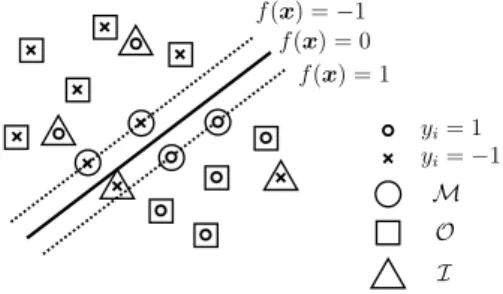
where O, M, and I stand for ‘Outside the margin’ (yif (xi)≥1), ‘on the Margin’
(yif (xi)=1), and ‘Inside the margin’ (yif (xi)≤1), respectively (see Fig.1). In (6a),
(6b), (6c), (6d) and (7a), (7b), (7c) we implicitly assumeCi>0. Since the data instancei
withCi=0 does not have any effect on the optimization problem, we do not need to take
into account such cases. The only exception is the case where data instances are added or removed using our proposed approach (for detail, see Sect.3.4).
In what follows, the subscript by an index set such asvI for a vectorv∈Rnindicates a sub-vector ofv whose elements are indexed byI. For example, forv=(a, b, c)and
I= {1,3},vI =(a, c). Similarly, the subscript by two index sets such asMM,O for a matrixM∈Rn×ndenotes a sub-matrix whose rows and columns are indexed byMandO,
Fig. 1 The partitioning of the
data points in SVM
3 Solution-path algorithm for WSVM
The path-following algorithm for the ordinary SVM (Hastie et al.2004) computes the entire solution path for the single regularization parameterC. In this section, we develop a path-following algorithm for the vector of weightsc= [C1, . . . , Cn]. Our proposed algorithm keeps track of the optimalαiandbwhen the weight vectorcis changed.
3.1 Analytic expression of WSVM solutions Let α= ⎡ ⎢ ⎣ α1 .. . αn ⎤ ⎥ ⎦, y= ⎡ ⎢ ⎣ y1 .. . yn ⎤ ⎥ ⎦, and Q= ⎡ ⎢ ⎣ Q11 · · · Q1n .. . . .. ... Qn1 · · · Qnn ⎤ ⎥ ⎦.
Then, using the index sets (7b) and (7c), we can expand one of the KKT conditions, (6b), as
QMαM+QM,IcI+yMb=1, (8)
where 1 denotes the vector with all ones. Similarly, another KKT condition (6d) is expressed as yMαM+yIcI=0. (9) Let M= 0 yM yM QM .
Then (8) and (9) can be compactly expressed as the following system of|M| +1 linear equations, where|M|denotes the number of elements in the setM:
M b αM + yI QM,I cI= 0 1 . (10)
Solving (10) w.r.t.bandαM, we obtain b αM = −M−1 yI QM,I cI+M−1 0 1 , (11)
where we implicitly assumed thatMis invertible.1Sincebandα
Mare affine w.r.t.cI, we can calculate the change ofband αMby (11) as long as the weight vectorcis changed continuously. By the definition ofIandO, the remaining parametersαIandαOare merely given by
αI=cI, (12)
αO=0. (13)
A change of the index setsM,O, andIis called an event. As long as no event occurs, the WSVM solutions for allccan be computed by (11)–(13) since all the KKT conditions (6a)–(6d) are still satisfied. However, when an event occurs, we need to check the violation of the KKT conditions. Below, we address the issue of event detection whencis changed. 3.2 Event detection
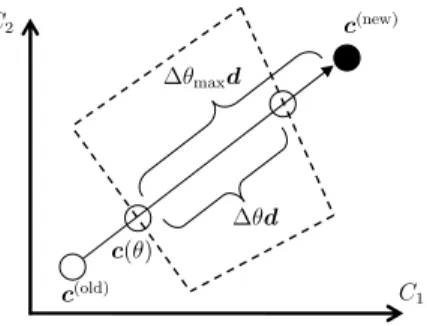
Suppose we want to change the weight vector fromc(old)toc(new)(see Fig.2). This can be
achieved by moving the weight vectorc(old)toward the direction ofc(new)−c(old).
Let us write the line segment betweenc(old)andc(new)in the following parametric form
c(θ )=c(old)+θc(new)−c(old), θ∈ [0,1],
whereθis a parameter. This parametrization allows us to derive a path-following algorithm between arbitraryc(old)andc(new)by considering the change of solutions whenθ is moved
from 0 to 1. This parametrization may also be interpreted as one-dimensional parametric programming with respect to the scalarθ, and our construction of the algorithm follows a similar line to one-dimensional regularization path algorithms. However, we will later il-lustrate that the above parametrization covers various important machine learning problems and greatly widens the applicability of the path-following approach.
Suppose we are currently atc(θ )on the path, and the current solution is(b,α). Let
c=θc(new)−c(old), θ≥0, (14)
where the operator represents the amount of change of each variable from the current value. Ifθis increased from 0, we may encounter a point at which some of the KKT con-ditions (6a)–(6c) do not hold. This can be checked by investigating the following conditions.
⎧ ⎪ ⎪ ⎨ ⎪ ⎪ ⎩ yif (xi)+yif (xi)≥1, i∈O, αi+αi>0, i∈M, αi+αi−(Ci+Ci, ) <0, i∈M, yif (xi)+yif (xi)≤1, i∈I. (15)
The set of inequalities (15) defines a convex polyhedron, called a critical region in the multi-parametric programming literature (Pistikopoulos et al.2007). The event points lie on the border of critical regions, as illustrated in Fig.2.
1The invertibility of the matrixM is assured if and only if the submatrixQ
Mis positive definite in the subspace{z∈R|M||yMz=0}. We assume this technical condition here. A notable exceptional case is thatMis empty—we will discuss how to cope with this case in detail in Sect.3.3.
Fig. 2 The schematic illustration of path-following in the space ofc∈R2, where the WSVM solution is updated fromc(old)toc(new). Suppose we are currently atc(θ ). The vectordrepresents the update direction
c(new)−c(old), and the polygonal region enclosed by dashed lines indicates the current critical region. Al-thoughc(θ )+θmaxdseems to directly lead the solution toc(new), the maximum possible update fromc(θ )
isθd; otherwise the KKT conditions are violated. To go beyond the border of the critical region, we need to update the index setsM,I, andOto fulfill the KKT conditions. When the solution path hits a corner of a critical region, the index sets cannot be uniquely defined. Such a case can be properly handled, e.g., by Bland’s rule, which is used to cope with degeneracy situations in linear/quadratic programming (Bland1977)
We detect an event point by checking the conditions (15) along the solution path as follows. Using (11), we can express the changes ofbandαMas
b αM =θφ, (16) where φ= −M−1 yI QM,I c (new) I −c(Iold) . (17) Furthermore,yif (xi)is expressed as yif (xi)= yiQi,M b αM +Qi,IcI =θ ψi, (18) where ψi= yiQi,M φ+Qi,IcI(new)−c(Iold). (19) Let us denote the elements of the index setMas
M= {m1, . . . , m|M|}.
Substituting (16) and (18) into the inequalities (15), we can obtain the maximum step-length with no event occurrence as
θ= min i∈{1,...,|M|},j∈I∪O −αmi φi+1 ,Cmi−αmi φi+1−dmi ,1−yjf (xj) ψj + , (20)
whereφi denotes the i-th element ofφ anddi=C( new) i −C
(old)
i . We used mini{zi}+as a
simplified notation of mini{zi|zi≥0}. Based on this largest possibleθ, we can compute
At the border of the critical region, we need to update the index setsM,O, andI. For example, ifαi (i∈M) reaches 0, we need to move the elementi fromMtoO. Then the
above path-following procedure is carried out again for the next critical region specified by the updated index setsM,O, andI, and this procedure is repeated untilcreachesc(new).
3.3 Empty margin
In the above derivation, we have implicitly assumed that the index setMis not empty— whenMis empty, we can not use (16) becauseM−1does not exist.
WhenMis empty, the KKT conditions (6a), (6b), (6c) and (6d) can be re-written as j∈I QijCj+yib≥1, i∈O, (21a) j∈I QijCj+yib≤1, i∈I, (21b) i∈I yiCi=0. (21c)
Although we can not determine the value ofb uniquely only from the above conditions, (21a) and (21b) specify the range of optimalb:
max i∈Lyigi≤b≤mini∈Uyigi, (22) where gi=1− j∈I QijCj, L= {i|i∈O, yi=1} ∪ {i|i∈I, yi= −1}, U= {i|i∈O, yi= −1} ∪ {i|i∈I, yi=1}. Let δ≡ i∈I yidi, where di=Ci(new)−C (old) i .
Whenδ=0, the step sizeθcan be increased as long as the inequality (22) is satisfied. Violation of (22) can be checked by monitoring the upper and lower bounds of the biasb (which are piecewise-linear w.r.t.θ) whenθis increased
u(θ )=max i∈U yi gi+gi(θ ) , (θ )=min i∈Lyi gi+gi(θ ) , (23)
where
gi(θ )= −θ
j∈I Qijdj.
On the other hand, whenδ=0,θ can not be increased without violating the equality condition (21c). In this case, an instance with index
ilow=arg max i∈L yigi or iup=arg min i∈U yigi
actually enters the index setM. If the instance (we denote its index bym) comes from the index setO, the following equation must be satisfied for keeping (21c) satisfied:
θ δ= −αmym.
Sinceθ >0 andαm>0, we have
sign(δ)=sign(−ym).
On the other hand, if the instance comes from the index setI, θ δ=ym(Cm−αm)
must be satisfied. Sinceθ >0 andCm−αm>0, we have
sign(δ)=sign(ym).
Considering these conditions, we arrive at the following updating rules forbandM: δ >0 ⇒ b=yiupgiup, M= {iup},
δ <0 ⇒ b=yilowgilow, M= {ilow}.
(24)
Note that we also need to removeiupandilowfromOandI, respectively. 3.4 Dealing withCi=0
WhenCi=0, the data instance(xi, yi)has no contribution to the optimization problem (3).
Therefore, we do not usually need to care about such a data instance. However, exploiting this fact, we can add and/or remove data instances using the proposed path algorithm: – To add a data instance(xi, yi), we increaseCifrom 0 to some specified value. To
imple-ment this idea, we first have to assign indexito one of the index setsM,IorO, but the definitions of the index sets (7a), (7b) and (7c) conflict whenCi=0. Here, we determine
the initial index set using the following rules:
yif (xi)=1 ⇒ i∈M,
yif (xi) <1 ⇒ i∈I.
After this initialization, we can follow the change of optimal solutions using the same procedure as we described so far.
– To remove a data instance(xi, yi), we decreaseCi to 0 from some initial value. In this
case, we do not need to consider the assignment of indexi, but we just remove(xi, yi)
from training data.
If we have a set of several data instances to add and remove, we can simply apply the above procedure simultaneously for those data instances (i.e., increase or decrease a set ofCi’s
simultaneously).
3.5 Computational complexity
The entire pseudo-code of the proposed WSVM path-following algorithm is described in Fig.3.
The computational complexity at each iteration of our path-following algorithm is the same as that for the ordinary SVM (i.e., the single-C formulation) (Hastie et al. 2004). Thus, our algorithm inherits a superior computational property of the original path-following algorithm.
The update of the linear system (17) from the previous one at each event point can be carried out efficiently withO(|M|2)computational cost based on the Cholesky
decompo-sition rank-one update (Golub and Van Loan1996) or the block-matrix inversion formula
(Schott2005). Thus, the computational cost required for identifying the next event point is O(n|M|).
It is difficult to state the number of iterations needed for complete path-following be-cause the number of events depends on the sensitivity of the model and the data set. Several empirical results suggest that the number of events linearly increases w.r.t. the data set size (Hastie et al.2004; Gunter and Zhu2007; Wang et al.2008); our experimental analysis given in Sect.4also showed the same tendency. This implies that path-following is com-putationally highly efficient—indeed, in Sect.4, we will experimentally demonstrate that the proposed path-following algorithm is faster than an alternative approach in one or two orders of magnitude.
4 Experiments
In this section, we illustrate the empirical performance of the proposed WSVM path-following algorithm in a toy example and two real-world applications. We compared the computational cost of the proposed path-following algorithm with the sequential
mini-mal optimization (SMO) algorithm (Platt1999) when the instance weights of WSVM are
changed in various ways. In particular, we investigated the CPU time of updating solutions from somec(old)toc(new).
In the path-following algorithm, we assume that the optimal parameter α and the Cholesky factorL ofQM forc(old)have already been obtained. In the SMO algorithm,
we used the old optimal parameterα as the initial starting point (i.e., the ‘hot’ start) after making them feasible using the alpha-seeding strategy (DeCoste and Wagstaff2000). We set the tolerance parameter in the termination criterion of SMO to 10−3. Our implemen-tation of the SMO algorithm is based on LIBSVM (Chang and Lin2011). To circumvent
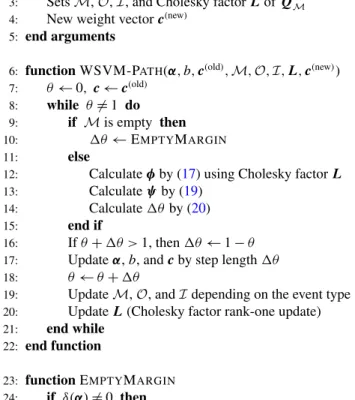
1: arguments:
2: Optimal parametersαandbforc(old) 3: SetsM,O,I, and Cholesky factorLofQM
4: New weight vectorc(new) 5: end arguments
6: function WSVM-PATH(α, b,c(old),M,O,I,L,c(new)) 7: θ←0,c←c(old)
8: while θ=1 do
9: if Mis empty then
10: θ←EMPTYMARGIN
11: else
12: Calculateφby (17) using Cholesky factorL
13: Calculateψby (19)
14: Calculateθby (20)
15: end if
16: Ifθ+θ >1, thenθ←1−θ
17: Updateα,b, andcby step lengthθ
18: θ←θ+θ
19: UpdateM,O, andIdepending on the event type
20: UpdateL(Cholesky factor rank-one update)
21: end while
22: end function
23: function EMPTYMARGIN 24: if δ(α)=0 then
25: Set bias termbby (24)
26: θ←0
27: else
28: Traceu(θ )and(θ )in (23) untilu(θ )=(θ )
29: end if
30: returnθ
31: end function
Fig. 3 Pseudo-code of the proposed WSVM path-following algorithm
possible numerical instability, we added small positive constant 10−6to the diagonals of the matrixQ. In all the experiments, we used the Gaussian kernel
Kx,x=exp −γ px−x 2 , (25)
whereγ is a hyper-parameter andpis the dimensionality ofx. In both the path algorithm and the SMO algorithm, the cache of the kernel matrix is inherited from previous solutions. 4.1 Illustrative example
First, we illustrate the behavior of the proposed path-following algorithm using an artificial data set. Consider a binary classification problem with the training set{(xi, yi)}ni=1, where
xi∈R2andyi∈ {−1,+1}. Let us define the sets of indices of positive and negative instances
asK−1= {i|yi= −1}andK+1= {i|yi= +1}, respectively. We assume that the loss function
is defined as i viI yif (xi)≤0 , (26)
wherevi∈ {1,2}is the cost of misclassifying the instance(xi, yi), andI (·)is the indicator
function. LetD1= {i|vi=1}andD2= {i|vi=2}, i.e.,D2is the set of instance indices that have stronger influence on the overall test error thanD1.
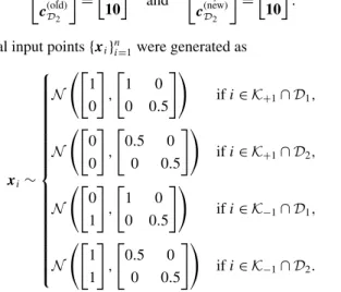
To be consistent with the above error metric, it would be natural to assign a smaller weightC1 for i∈D1 and a larger weightC2 fori∈D2 when training SVM. However, naively settingC2=2C1 is not generally optimal because the hinge loss is used in SVM training, while the 0-1 loss is used in performance evaluation (see (26)). In the following experiments, we fixed the Gaussian kernel width toγ=1 and the instance weight forD2to C2=10, and we changed the instance weightC1forD1from 0 to 10. Thus, the change of the weights is represented as
c(Dold1) c(Dold2) = 0 10 and c(Dnew1 ) c(Dnew2 ) = 10 10 . Two-dimensional input points{xi}n
i=1were generated as xi∼ ⎧ ⎪ ⎪ ⎪ ⎪ ⎪ ⎪ ⎪ ⎪ ⎪ ⎪ ⎪ ⎪ ⎪ ⎪ ⎪ ⎪ ⎪ ⎨ ⎪ ⎪ ⎪ ⎪ ⎪ ⎪ ⎪ ⎪ ⎪ ⎪ ⎪ ⎪ ⎪ ⎪ ⎪ ⎪ ⎪ ⎩ N 1 0 , 1 0 0 0.5 ifi∈K+1∩D1, N 0 0 , 0.5 0 0 0.5 ifi∈K+1∩D2, N 0 1 , 1 0 0 0.5 ifi∈K−1∩D1, N 1 1 , 0.5 0 0 0.5 ifi∈K−1∩D2. (27)
Figure4shows the generated instances forn=400, with the equal sizen/4 for the above four cases. Before feeding the generated instances into algorithms, we normalized the inputs in[0,1]2.
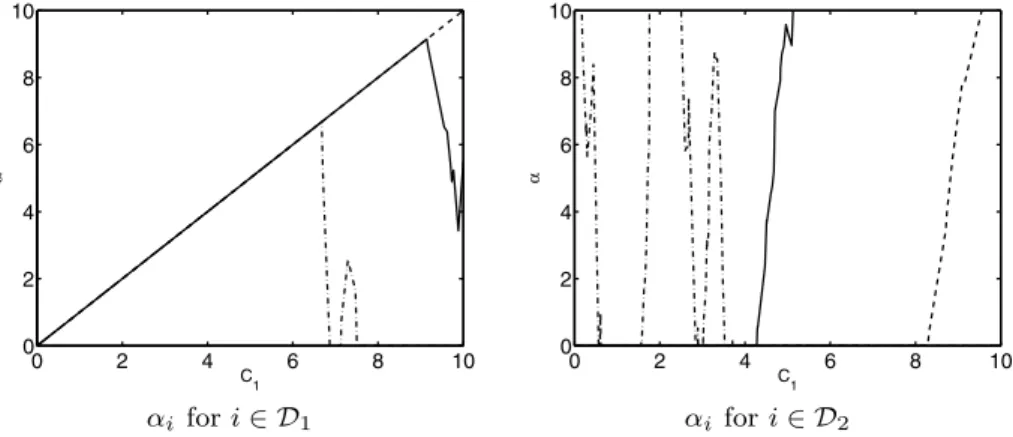
Figure5illustrates piecewise-linear paths of the solutionsαiforC1∈ [0,10]whenn= 400. The left graph includes the solution paths of three representative parametersαi for
i∈D1. All three parameters increase as C1 grows from zero, and one of the parameters (denoted by the dash-dotted line) suddenly drops down to zero at aroundC1=7. Another parameter (denoted by the solid line) also sharply drops down at aroundC1=9, and the last one (denoted by the dashed line) remains equal toC1untilC1reaches 10. The right graph includes the solution paths of three representative parametersαi fori∈D2, showing that their behavior is substantially different from that forD1. One of the parameters (denoted by the dash-dotted line) fluctuates significantly, while the other two parameters (denoted by the solid and dashed lines) are more stable and tend to increase asC1grows.
An important advantage of the path following algorithm is that the path of the validation error can be traced as well (see Fig.6). First, note that the path of the validation error (26)
Fig. 4 Artificial data set generated by the distribution (27). The crosses and circles indicate the data points in
K−1(negative class) andK+1(positive class), respectively. The left plot shows the data points inD1(their
misclassification cost is 1), the middle plot shows the data points inD2(their misclassification cost is 2), and
the right plots show their union
Fig. 5 Examples of piecewise-linear paths ofαi for the artificial data set. The weights are changed from
Ci=0 to 10 fori∈D1(fori∈D2, the weights are fixed toCi=10). The left and right plots show the paths of three representative parametersαifori∈D1, and fori∈D2, respectively
has a piecewise-constant form because the 0–1 loss changes only when the sign of f (x) changes. In our path-following algorithm, the path off (x)also has a piecewise-linear form becausef (x) is linear w.r.t. their parametersα andb. Exploiting the piecewise linearity off (x), we can exactly detect the point at which the sign off (x)changes. These points correspond to breakpoints of the piecewise-constant validation-error path. Figure6 illus-trates the relationship between the piecewise-linear path off (x)and the piecewise-constant validation-error path. Figure7shows an example of piecewise-constant validation-error path whenC1is increased from 0 to 10, indicating that the lowest validation error was achieved at aroundC1=4.
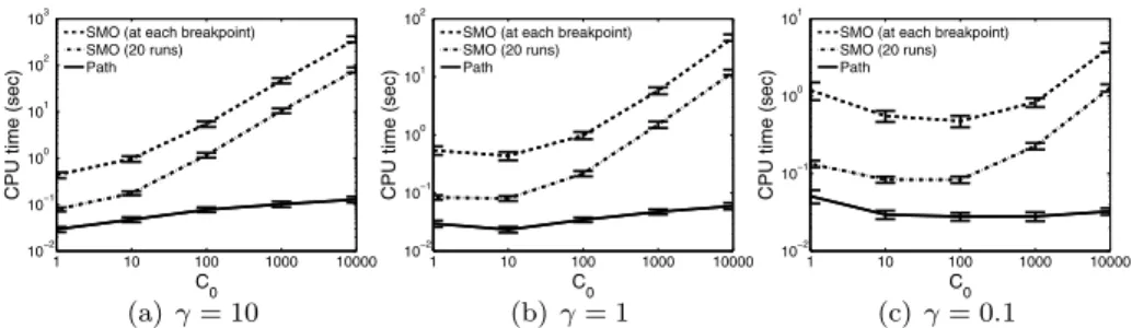
Finally, we investigated the computation time when the solution path fromC1=0 to 10 was computed. For comparison, we also investigated the computation time of the SMO algorithm run at every breakpoint and with 20 C1 values uniformly taken in log 10 scale from[0.1,1]. We considered the following four cases: the number of training instances was n=400, 800, 1200, and 1600. For eachn, we generated 10 data sets and the average and standard error over 10 runs are reported. Table1 describes the results, showing that the proposed path-following algorithm is faster than SMO run at every breakpoint in one or two
Fig. 6 A schematic illustration of validation-error path. In this plot, the path of misclassification error rate 1
3 n
i=1I (yif (xi))≤0)for the 3 validation instances(x1, y1),(x2, y2), and(x3, y3)are depicted. The hori-zontal axis indicates the parameterθand the vertical axis denotesyif (xi),i=1,2,3. The path of the valida-tion error has a piecewise-constant form because the 0-1 loss changes only whenf (xi)=0. The breakpoints of the piecewise-constant validation-error path can be exactly detected by exploiting the piecewise linearity off (xi)
Fig. 7 An example of the
validation-error path for 1000 validation instances of the artificial data set. The number of training instances is 400 and the Gaussian kernel withγ=1 is used
Table 1 The experimental results for the artificial data set. The average and the standard error (in brackets)
over 10 runs are reported. Here, SMO (BP) and SMO (20 runs) denotes the SMO algorithms run at every breakpoint and with 20C1values uniformly taken in log 10 scale from[0.1,1], respectively
n CPU time (sec.) #events mean|M|
path SMO (BP) SMO (20 runs)
400 0.02 (0.00) 0.39(0.01) 0.04 (0.00) 326.70(7.17) 3.07 (0.03) 800 0.06 (0.00) 2.87(0.12) 0.14 (0.00) 635.30(17.47) 3.27 (0.02) 1200 0.14 (0.01) 10.52(0.38) 0.32 (0.00) 997.60(26.85) 3.38 (0.05) 1600 0.26 (0.01) 27.72(0.76) 0.59 (0.01) 1424.00(31.27) 3.50 (0.02)
orders of magnitude and the difference becomes more significant as the training data sizen grows. The results also showed that the path approach was faster than SMO run at 20 points. The table also includes the number of events and the average number of elements in the margin setM(see (7b)). This shows that the number of events increases almost linearly w.r.t. the sample sizen, which well agrees with the empirical results reported in Hastie et al. (2004), Gunter and Zhu (2007), and Wang et al. (2008). The average number of elements in the setMincreases mildly as the sample sizengrows.
Fig. 8 The weight functions for
financial time-series
forecasting (Cao and Tay2003). The horizontal axis is the index of training instances sorted according to time (the most recent instance isi=n). If we set
a=0, all the instances are weighted equally
Fig. 9 A schematic illustration of the change of weights in time-series learning. The left plot shows the
fact that larger weights are assigned to more recent instances. The right plot describes a situation where we receive a new instance (i=n+1). In this situation, the oldest instance (i=1) is deleted by setting its weight to zero, the weight of the new instance is set to be the largest, and the weights of the rest of the instances are decreased accordingly
4.2 Online time-series learning
In online time-series learning, it is natural to assign larger (resp. smaller) weights to newer (resp. older) instances. For example, in Cao and Tay (2003), the following weight function is used: Ci=C0 2 1+exp(a−2a× i n) , (28)
where C0 and a are hyper-parameters and the instances are assumed to be sorted along the time axis (the most recent instance isi=n). Figure8shows the profile of the weight function (28) whenC0=1. In this online learning scheme, we need to update parameters when new observations arrive, and all the weights must be updated accordingly (see Fig.9). We investigated the computational cost of updating parameters when several new ob-servations arrive. The experimental data are obtained from the NASDAQ composite index between January 2, 2001 and December 31, 2009. As Cao and Tay (2003) and Chen et al. (2006), we transformed the original closing prices using the Relative Difference in Percent-age (RDP) of the price and the exponential moving averPercent-age (EMA).
Table 2 Features for financial
forecasting (p(i)is the closing price of theith day and EMAk(i) is thek-day exponential moving average of theith day)
Feature Formula
EMA15 p(i)−EMA15(i)
RDP-5 (p(i)−p(i−5))/p(i−5)∗100 RDP-10 (p(i)−p(i−10))/p(i−10)∗100 RDP-15 (p(i)−p(i−15))/p(i−15)∗100 RDP-20 (p(i)−p(i−20))/p(i−20)∗100 RDP+5 (p(i+5)−p(i))/p(i)∗100
p(i)=EMA3(i)
Fig. 10 CPU time comparison for online time-series learning with the NASDAQ composite index. The
optimalC0andγin terms of 10-fold cross-validation error (using the 0-1 loss) areC0=100 andγ=0.1 Extracted features are listed in Table2(see Cao and Tay2003, for more details). Our task is to predict the sign of RDP+5 using EMA15 and four lagged-RDP values (RDP-5, RDP-10, RDP-15, and RDP-20). RDP values that exceed±2 standard deviations are replaced with the closest marginal values. We have an initial set of training instances with sizen=2515. The inputs were normalized in[0,1]p, wherepis the dimensionality of the inputx. We used
the Gaussian kernel (25) withγ ∈ {10,1,0.1}, and the weight parameterain (28) was set to 3. We first trained WSVM using the initial set of instances. Then we added 5 instances to the previously trained WSVM and removed the oldest 5 instances by decreasing their weights to 0. This does not change the size of the training data set, but the entire weights need to be updated as illustrated in Fig.9. We iterated this process 5 times and compared the total computational costs of the path-following algorithm and the SMO algorithm. The cache of the kernel matrix is inherited from previous solutions at each update.
Figure 10shows the average CPU time and its standard error over 10 runs for C0∈ {1,10,102,103,104}, showing that the path-following algorithm is much faster than the SMO algorithm especially for largeC0.
4.3 Model selection in covariate shift adaptation
Covariate shift is a situation in supervised learning where input distributions change between training and test phases but the conditional distribution of outputs given inputs remains unchanged (Shimodaira2000). Under covariate shift, standard SVM and SVR are biased, and the bias caused by covariate shift can be asymptotically canceled by weighting the loss function according to the importance (i.e., the ratio of training and test input densities).
Here, we apply importance-weighted SVMs to brain-computer interfaces (BCIs) (Dorn-hege et al.2007). A BCI is a system that allows for a direct communication from man
Fig. 11 CPU time comparison for covariate shift adaptation using BCI data. The optimalC0andγin terms
of the validation error (using the 0-1 loss) areC0=100 andγ=1
to machine via brain signals. Strong non-stationarity effects have been often observed in brain signals between training and test sessions, which could be modeled as covariate shift (Sugiyama et al.2007). We used the BCI datasets provided by the Berlin BCI group (Burde and Blankertz 2006), containing 24 binary classification tasks. The input features are 4-dimensional preprocessed electroencephalogram (EEG) signals, and the output labels cor-respond to the ‘left’ and ‘right’ commands. The size of training datasets is around 500 to 1000, and the size of validation datasets is around 200 to 300.
Although the importance-weighted SVM tends to have lower bias, it in turns has larger estimation variance than the ordinary SVM (Shimodaira2000). Thus, in practice, it is de-sirable to slightly ‘flatten’ the instance weights so that the trade-off between bias and vari-ance is optimally controlled. Here, we changed the instvari-ance weights from the uniform val-ues to the importance valval-ues using the proposed path-following algorithm, i.e., the instance weights were changed fromCi(old)=C0toCi(new)=C0pptest(xi)
train(xi),i=1, . . . , n. The importance values ptest(xi)
ptrain(xi)were estimated by the method proposed in Kanamori et al. (2009), which di-rectly estimates the density ratio without going through density estimation ofptest(x)and ptrain(x).
For comparison, we ran the SMO algorithms at (i) each breakpoint of the solution path, and (ii) 20 weight vectors taken uniformly in[Ci(old), Ci(new)]. We normalized the inputs in
[0,1]pwherepis the dimensionality ofx, and used the Gaussian kernel.
Figure11shows the average CPU time and its standard error. We examined several set-tings of hyper-parameters γ ∈ {10,1, . . . ,10−2} and C
0∈ {1,10,102, . . . ,104}. The hori-zontal axis of each plot representsC0. The graphs show that our path-following algorithm is faster than the SMO algorithms in all cases. While the SMO algorithm tended to take longer time for largeC0, the CPU time of the path-following algorithm did not increase as C0increases.
5 Beyond classification
So far, we focused on classification scenarios. Here we show that the proposed path-following algorithm can be extended to various scenarios including regression, ranking, and transduction.
5.1 Regression
The support vector regression (SVR) is a variant of SVM for regression problems (Vap-nik et al.1996; Mattera and Haykin1999; Müller et al.1999). For SVR, several solution
path algorithms have been considered (Gunter and Zhu2007; Wang et al.2008). However, they only deal with one or two hyper-parameters to change. Here, we briefly show that our approach can be applicable to a weighted variant of SVR using the same technique as we described so far.
5.1.1 Formulation
The primal optimization problem for the weighted SVR (WSVR) is defined by
min w,b,{ξi,ξi∗} n i=1 1 2w 2 2+ n i=1 Ci ξi+ξi∗ , s.t. yi−f (xi)≤ε+ξi, f (xi)−yi≤ε+ξi∗, ξi, ξi∗≥0, i=1, . . . , n,
where >0 is the insensitive-zone thickness. Note that, as in the classification case, WSVR is reduced to the original SVR whenCi=Cfori=1, . . . , n. Thus, WSVR includes SVR
as a special case.
The corresponding dual problem is given by
max {αi}ni=1 −1 2 n i=1 n j=1 αiαjK(xi,xj)−ε n i=1 |αi| + n i=1 yiαi s.t. n i=1 αi=0, −Ci≤αi≤Ci, i=1, . . . , n.
The final solution, i.e., the regression functionf:X→R, is in the following form: f (x)=
n
i=1
αiK(x,xi)+b.
The KKT conditions for the above dual problem are given as
|yi−f (xi)| ≤ε, ifαi=0, (29a) |yi−f (xi)| =ε, if 0<|αi|< Ci, (29b) |yi−f (xi)| ≥ε, if|αi| =Ci, (29c) n i=1 αi=0. (29d)
Then the training instances can be partitioned into the following three index sets (see Fig.12): O=i: |yi−f (xi)| ≥ε,|αi| =Ci , E=i: |yi−f (xi)| =ε,0<|αi|< Ci ,
Fig. 12 Partitioning of data points in SVR I=i: |yi−f (xi)| ≤ε, αi=0 . Let KE= 0 1 1 KE and s= ⎡ ⎢ ⎣ sign(y1−f (x1)) .. . sign(yn−f (xn)) ⎤ ⎥ ⎦. Then, from (29a), (29b), (29c) and (29d) we obtain
b αE = −KE−1 1O KE,O diag(sO)cO+KE−1 0 yE−εsE , αO=diag(sO)cO, αI=0,
where diag(sO)indicates the diagonal matrix with diagonal elements given bysO. Because these functions are affine w.r.t.c, we can easily detect an event by monitoring the inequalities in (29a), (29b), (29c) and (29d). We can follow the solution path of SVR by using essentially the same technique as SVM classification (and thus the details are omitted).
5.1.2 Experiments on regression
As an application of WSVR, we consider a heteroscedastic regression problem, where output noise variance depends on input points. In heteroscedastic data modeling, larger (resp. smaller) weights are usually assigned to instances with smaller (resp. larger) vari-ances. Because the point-wise variances are often unknown in practice, they should also be estimated from data. A standard approach is to alternately estimate the weight vector cbased on the current WSVR solution and update the WSVR solutions based on the new weight vectorc(Kersting et al.2007).
We set the weights as
Ci=C0
σ
|ei|, (30)
whereei=yi−f (x i)is the residual of the instance(xi, yi)from the current fitf (x i), andσ
is an estimate of the common standard deviation of the noise computed asσ= n1ni=1ei2. We employed the following procedure for the heteroscedastic data modeling:
Fig. 13 Comparison of CPU time for heteroscedastic modeling on the Boston housing data. The optimalC0
andγin terms of the validation error (using the squared loss) areC0=10000 andγ=0.1
Fig. 14 The number of weight updates for the Boston housing data
Step 2: Update weights by (30) and update the solution of WSVR accordingly. Repeat this step until1nni=1|(ei(old)−ei)/ei(old)| ≤10−3holds, wheree(old)is the previous
train-ing error.
We investigated the computational cost of Step 2. We applied the above procedure to the Boston housing data set. The sample size is 506 and the number of features isp=13. The inputs were normalized in[−1,1]p. We randomly sampledn=404 instances for SVR
training from the original data set, and the experiments were repeated 10 times. We used the Gaussian kernel (25) withγ ∈ {10,1,0.1}. The insensitive-zone thickness in WSVR was fixed toε=0.05.
Each plot of Fig. 13 shows the average CPU time and standard error for C0 ∈ {1,10, . . . ,104}, and Fig.14 shows the number of repetitions performed in Step 2. This shows that our path-following approach is faster than the SMO algorithm especially for largeC0.
5.2 Ranking
Recently, the problem of learning to rank has attracted wide interest as a challenging topic in machine learning and information retrieval (Liu2009). Here, we focus on a method called the ranking SVM (RSVM) (Herbrich et al.2000). RSVM learns a ranking model using a similar formulation to SVM. Arreola et al. (2008) derived the regularization path algorithm for RSVM. In this subsection, we describe that an instance-weighting strategy is useful in the ranking task and our solution path approach can be applied to the weighted variant of RSVM.
5.2.1 Formulation
Assume that we have a set ofntriplets{(xi, yi, qi)}ni=1wherexi∈Rpis a feature vector of
an item andyi∈ {r1, . . . , rq}is a relevance ofxi to a queryqi. The relevance has an order
of the preferencerqrq−1 · · · r1, whererqrq−1means thatrqis preferred torq−1. The goal is to learn a ranking functionf (x)that returns a larger value for a preferred item. More precisely, for itemsxiandxj such thatqi=qj, we want the ranking functionf (x)to
satisfy
yiyj ⇔ f (xi) > f (xj).
Let us define the following set of pairs:
P=(i, j )|yiyj, qi=qj
. RSVM solves the following optimization problem:
min w,{ξij}(i,j )∈P 1 2w 2 2+C (i,j )∈P ξij s.t. f (xi)−f (xj)≥1−ξij, (i, j )∈P.
In practical ranking tasks such as information retrieval, it is natural that a pair of items with highly different preference levels has a larger weight than that with similar preference levels. Based on this prior knowledge, Cao et al. (2006) and Xu et al. (2006) proposed to assign different weightsCij to different relevance pairs(i, j )∈P. This is a cost-sensitive
variant of RSVM whose primal problem is given as
min w,{ξij}(i,j )∈P 1 2w 2 2+ (i,j )∈P Cijξij s.t. f (xi)−f (xj)≥1−ξij, (i, j )∈P.
Because this formulation is interpreted as a WSVM for pairs of items(i, j )∈P, we can use our path approach. Note that the solution path algorithm for the cost-sensitive RSVM is regarded as an extension of Arreola et al. (2008), in which the solution path for the standard RSVM was studied.
Now, let us consider a model selection problem for the weighting pattern{Cij}(i,j )∈P. We assume that the weighting pattern is represented as
Cij=C( old) ij +θ
Cij(new)−Cij(old), (i, j )∈P, θ∈ [0,1], (31) where
Cij(old)=C0, (i, j )∈P, (32)
Cij(new)=2yi−2yjC
Fig. 15 The schematic
illustration of the NDCG path. The upper plot shows outputs for 3 items which have different levels of preferencesy. The
bottom plot shows the changes of
the NDCG. Since the NDCG depends on the sorted order of items, it changes only when two
lines of the upper plot intersect
andC0is the common regularization parameter.2We follow the multi-parametric solution path from{Cij(old)}(i,j )∈Pto{C(ijnew)}(i,j )∈P and the bestθis selected based on the validation
performance.
The performance of ranking algorithms is usually evaluated by some information-retrieval measures such as the normalized discounted cumulative gain (NDCG) (Järvelin and Kekäläinen2000). Consider a queryq and defineq(j )as the index of thej-th largest item among{f (xi)}i∈{i|qi=q}. The NDCG at positionkfor a queryqis defined as
NDCG@k=Z k j=1 ! 2yq(j )−1, j=1, 2yq(j)−1 log(j ) , j >1, (34)
whereZis a constant to normalize the NDCG in[0,1]. Note that the NDCG value in (34) is defined using only the topkitems and the rest are ignored. The NDCG for multiple queries are defined as the average of (34).
The goal of our model selection problem is to chooseθ with the largest NDCG value. As explained below, we can identifyθthat attains the exact maximum NDCG value for val-idation samples by exploiting the piecewise linearity of the solution path. The NDCG value changes only when there is a change in the topkranking, and the rank of two itemsxiand
xjchanges only whenf (xi)andf (xj)cross. Then change points of the NDCG can be
ex-actly identified becausef (x)changes in a piecewise-linear manner. Figure15schematically illustrates piecewise-linear paths and the corresponding NDCG path for validation samples. The validation NDCG changes in a piecewise-constant manner, and change points are found when there is a crossing between two piecewise-linear paths.
5.2.2 Experiments on ranking
We used the OHSUMED data set included in the LETOR package (version 3.0) provided by Microsoft Research Asia (Liu et al.2007). We used the query-level normalized version of the data set containing 106 queries. The total number of query-document pairs is 16140, and the number of features isp=45. The data set provided is originally partitioned into 5 subsets, each of which has training, validation, and test sets for 5-fold cross validation. Here, we only used the training and the validation sets.
2In Chapelle and Keerthi (2010), ranking of each item is also incorporated to define the weighting pattern.
However, these weights depend on the current ranking, and it might change during training. We thus, for simplicity, introduce the weighting pattern (33) that depends only on the difference of the preference levels.
Fig. 16 CPU time comparison for RSVM. The optimalC0andγin terms of validation NDCG areC0=0.01
andγ=1
Fig. 17 The number of instances
on the margin|M|in ranking experiment
We compared the CPU time of our path algorithm and the SMO algorithm to change
{Cij}(i,j )∈P from the flat weight pattern (32) to the relevance weight pattern (33). We need to modify the SMO algorithm to train the model without the explicit bias termb. The usual SMO algorithm updates two selected parameters per iteration to ensure that the solution satisfies the equality constraint derived from the optimality condition ofb. Since RSVM has no bias term, the algorithm is adapted to update one parameter per iteration (Vogt2002). We employed the update rule of Vogt (2002) to adapt the SMO algorithm to RSVM and we chose the maximum violating point as the parameter to update. This strategy is analogous to the maximum violating-pair working set selection of Keerthi et al. (2001) in ordinary SVM. Since it took relatively large computation time, we ran the SMO algorithm only at 10 points uniformly taken in[Cij(old), Cij(new)]. We considered every pair of initial weightC0∈ {10−5, . . . ,10−1} and Gaussian width γ ∈ {10,1,0.1}. The results, given in Fig. 16 (the average CPU time and its standard error), show that the path algorithm is faster than the SMO in all of the settings.
The CPU time of the path algorithm in Fig.16(a) increases asC0increases because the number of breakpoints and the size of the setMalso increase. Since our path algorithm solves a linear system with size|M|usingO(|M|2)update in each iteration, practical com-putational time depends on|M|especially in large data sets. In the case of RSVM, the max-imum value of|M|is the number of pairs of training documentsm= |P|. For each fold of the OHSUMED data set,m=367663, 422716, 378087, 295814, and 283484. If|M| ≈m, a large computational cost may be needed for updating the linear system. However, as Fig.17 shows, the size|M|is at most about one hundred in this setup.
Figure18 shows the example of the path of validation NDCG@10. Since the NDCG depends on the sorted order of documents, direct optimization is rather difficult (Liu2009). Using our path algorithm, however, we can detect the exact behavior of the NDCG by
mon-Fig. 18 The change of
NDCG@10 forγ=0.1 and
C=0.01. The parameterθin the
horizontal axis is used as
c(old)+θ (c(new)−c(old))
itoring the change of scores f (x) in the validation data set. Then we can find the best weighting pattern by choosingθ with the maximum NDCG for the validation set.
5.3 Transduction
In transductive inference (Vapnik1995), we are given unlabeled instances along with la-beled instances. The goal of transductive inference is not to estimate the true decision func-tion, but to classify the given unlabeled instances correctly. The transductive SVM (TSVM) (Joachims1999) is one of the most popular approaches to transductive binary classification. The objective of the TSVM is to maximize the classification margin for both labeled and unlabeled instances.
5.3.1 Formulation
Suppose we have k unlabeled instances {x∗i}k
i=1 in addition to n labeled instances {(xi, yi)}ni=1. The optimization problem of TSVM is formulated as
min {yi∗,ξi∗}k i=1,w,b,{ξi}ni=1 1 2w 2 2+C n i=1 ξi+C∗ k j=1 ξj∗ (35) s.t. yi(wΦ(xi)+b)≥1−ξi, i=1, . . . , n, yj∗(wΦ(xj)+b)≥1−ξj∗, j=1, . . . , k, ξi≥0, i=1, . . . , n, ξj∗≥0, j=1, . . . , k,
whereCandC∗are the regularization parameters for labeled and unlabeled data, respec-tively, andyj∗∈ {−1,+1}, j=1, . . . , k, are the labels of the unlabeled instances{x∗i}k
i=1. Note that (35) is a combinatorial optimization problem with respect to{yj∗}j∈{1,...,k}. The
op-timal solution of (35) can be found if we solve binary SVMs for all possible combinations of
{y∗j}j∈{1,...,k}, but this is computationally intractable even for moderatek. To cope with this
problem, Joachims (1999) proposed an algorithm that approximately optimizes (35) by solv-ing a series of WSVMs. The subproblem is formulated by assignsolv-ing temporarily estimated labelsyj∗to unlabeled instances:
min {ξi∗}ki=1,w,b,{ξi}ni=1 1 2w 2 2+C n i=1 ξi+C−∗ j∈{j|yj∗=−1} ξj∗+C+∗ j∈{j|yj∗=1} ξj∗ (36)
s.t. yi(wΦ(xi)+b)≥1−ξi, i=1, . . . , n, yj∗(wΦ(xj)+b)≥1−ξj∗, j=1, . . . , k, ξi≥0, i=1, . . . , n, ξj∗≥0, j=1, . . . , k,
whereC∗−andC+∗ are the weights for unlabeled instances{j|yj∗= −1}and{j|yj∗= +1}, respectively. The entire algorithm is given as follows (see Joachims1999, for details): Step 1: Set the parametersC,C∗, andk+, wherek+is defined as
k+=k×|{j|yj= +1, j=1, . . . , n}|
n .
k+is defined so that the balance of positive and negative instances in the labeled set is equal to that in the unlabeled set.
Step 2: Optimize the decision function using only the labeled instances and compute the decision function values{f (x∗j)}k
j=1. Assign the positive labelyj∗=1 to the topk+
unlabeled instances in decreasing order off (x∗j), and the negative labely∗j= −1 to the remaining instances. SetC−∗ andC+∗ to some small values (see Joachims1999, for details).
Step 3: Train SVM using all the instances (i.e., solve (36)). Switch the labels of a pair of positive and negative unlabeled instances if the objective value (35) is reduced, where the pair of instances is selected based on{ξj∗}j∈{1,...,k}(see Joachims1999,
for details). Iterate this step until no data pair decreases the objective value. Step 4: SetC−∗ =min(2C−∗, C∗)andC+∗=min(2C+∗, C∗). IfC−∗ ≥C∗andC+∗≥C∗,
termi-nate the algorithm. Otherwise return to Step 3.
Our path-following algorithm can be applied to Steps 3 and 4 for accelerating the above TSVM algorithm. Step 3 can be carried out via path-following as follows:
Step 3(a) Choose a pair of positive instancex∗mand negative instancex∗m.
Step 3(b) After removing the positive instancex∗mby decreasing its weight parameterCm
fromC+∗ to 0, add the instancex∗mas a negative one by increasingCmfrom 0
toC−∗.
Step 3(c) After removing the negative instancex∗mby decreasing its weight parameterCm
fromC−∗ to 0, add the instancex∗m as a positive one by increasingCm from 0
toC+∗.
Note that the label switching in Steps 3(b) and 3(c) may be merged into a single step. Step 4 also can be carried out by our path-following algorithm.
5.3.2 Experiments on transduction
We compare the computation time of the proposed path-following algorithm and the SMO algorithm for Steps 3 and 4 of the TSVM algorithm. We used the spam data set obtained from the UCI machine learning repository (Asuncion and Newman2007). The sample size is 4601, and the number of features isp=57. We randomly selected 10 % of data points as labeled instances, and the remaining 90 % were used as unlabeled instances. The inputs were normalized in[0,1]p.
Figure19shows the average CPU time and its standard error over 10 runs for the Gaus-sian widthγ ∈ {10,1,0.1}andC∈ {1,10,102, . . . ,104}. The figure shows that our algo-rithm is consistently faster than the SMO algoalgo-rithm in all of these settings.