Optimal Functionality Placement for
Multiplay Service Provider Architectures
Ioannis Papapanagiotou,
Student Member, IEEE
, Matthias Falkner,
Member, IEEE
,
and Michael Devetsikiotis,
Fellow, IEEE
Abstract—The proliferation of multiplay services is creating
design dilemmas for service providers, related to where certain key networking functionality should be placed. For example, service providers need to know whether to distribute more network intelligence closer to the subscriber or cluster it in a central location. In view of this, we quantify the cost differences among service provider architectures, identified based on the functionality distribution (centralized vs. distributed, clustered vs. unclustered and single vs. multi edge). For this purpose, we formulate a modular mixed-integer programming model based on a set of close-to-real-case scenarios. Given the complexity of such problems, we propose methodologies that can reduce the number of locations. Our results indicate that distributing the IP intelligence and the video replication is preferable. Moreover, deploying edge systems with faster backplane has little benefit in the aggregation network, and providers should rather invest in faster interfaces.
Index Terms—Aggregation networks, metro Ethernet, Ethernet
based DSL, edge systems, triple play.
I. INTRODUCTION
T
HE well established 80/20 rule for client-server versus local traffic has driven network designers to address problems with pure L2 switches acting as hubs, and L3 routers performing the routing towards different paths. However, the rise of on demand video streaming (e.g., Netflix, Hulu), Peer-to-Peer (P2P) television over the internet (e.g., TVUPlayer, PPLive, QQLive, PPStream), and the advent of mobile traffic has triggered a number of actions from broadband providers who are trying to achieve flexibility, scalability and efficiency [21]. According to several studies, the annual global traffic will be doubling in volume every two years, while a quarter of this is projected to be video traffic [2], [3]. Current 4G mobile service provider architectures are bandwidth constrained, and the cost to build out new networks to increase the available bandwidth is prohibitively expensive.Therefore, it is of vital importance for the Internet Service Providers (ISPs) to engineer their infrastructure to meet these challenges. In this paper, we focus on answering the question Manuscript received March 5, 2011; revised November 28, 2011, and March 15 and May 29, 2012. The associate editor coordinating the review of this paper and approving it for publication was A. Vasilakos.
I. Papapanagiotou and M. Devetsikiotis are with the Department of Electri-cal and Computer Engineering, North Carolina State University, Raleigh NC, 27606 USA (e-mail:{ipapapa, mdevets}@ncsu.edu).
M. Falkner is with the Edge Router Business Unit of Cisco Systems, Ottawa, Canada (e-mail: [email protected]).
This work was supported in part by the Institute for Next Generation IT Systems, Research Grant 09-06, and by the Cisco University Research Program, Gift #2008-04555 (3696).
Digital Object Identifier 10.1109/TNSM.2012.061212.110032
of where to place certain functionalities in the aggregation
network. We model this through a Network Design Problem (NDP) that the SP may use to achieve the maximum efficiency with the minimum deployment capital cost.
In the past, NDPs have been used to address the problem of cost optimization when developing new infrastructures. Nonetheless, most ISPs already possess an access infrastruc-ture. In order to address this issue, we propose an optimization formulation that uses the current infrastructure (in terms of design), but defines the optimal distribution offunctionalities
instead. Another important aspect is that devices used in the Ethernet aggregation, and edge part of the network, are not anymore purely layer 2 switches (in the NDP literature they are sometimes called “aggregators” [26]) and layer 3 routers. Most of the vendors have engineered multipurpose edge “systems” that incorporate different functionalities and network intelligence in modular “sub-systems” e.g., high-end backplanes in which multiple interface and functionality line cards are added. Therefore, design problems for such architectures need to be revisited.
Considering the above challenges, in this paper we classify the aggregation architectures based on the location of the functionalities and network intelligence, and then proceed to build a modular optimization model that is able to achieve the minimum deployment cost. Our contribution is summarized as follows:
• We define the possible aggregation architectures and group them into three main categories: 1. Centralized
Single-Edge; 2. Centralized Multi-Edge; and 3.
Dis-tributed Single-Edge. On top of these categories, another
subcategory is added, whether to cluster the edge systems or keep the functionalities in a single box.
• We develop a network design model that goes beyond the well investigated location and dimensioning problems. Our modeling approach is applied to both design an aggregation architecture, as well as upgrading the current infrastructure.
• We propose models based on edge “systems”, rather than network elements. Edge systems may support different types of functionalities either on their own, or as attached “sub-systems” (line cards).
• We formulate constraints that account for physical char-acteristics (line card capacity, port capacity), bandwidth (device and port bandwidth), and layer 2 versus layer 3 functionalities (such as switching and routing, VLAN/IP termination capacity, or business functions).
• We propose two novel heuristics for scaling down the problem and for decreasing the execution time of the problem.
• We evaluate our model with two close-to-real-case sce-narios and with multiple traffic profiles. We show that, with the current trends, the SPs will need to re-engineer their aggregation infrastructure.
The paper is structured as follows: In the next section, we provide an overview of the current state of the art in NDPs and aggregation design methodologies. In section III, we define and explain the architectures according to the distribution of the edge systems. In section IV, we describe the proposed modeling methodology and assumptions. Given the plurality of symbols and notations, all of them are summarized in the tables of section IV. In section V, we explain the modeling approach for the traffic flows and in Section VI we deploy the cost optimization model. In section VII, we explain the heuristics that have been used to scale-down the problem, and in section VIII we showcase an evaluation of two multi-service scenarios over metro area networks based on architectural values from EU ISPs and actual system values from vendors. Section IX, includes the discussion and further remarks, and we conclude with the final section.
II. BACKGROUNDWORK
During the Internet era the extensive need for bandwidth became a crucial issue for Internet SPs. This led the research community to focus on Network Design Problems that require advanced optimization techniques to be solved. These prob-lems can be divided into two main categories: Locationing
problems, which are pure topological design problems and
where the demand volumes are not taken into considera-tion; Dimensioning problems, which incorporate the demand volumes. Both classes of problems have been extensively analyzed in [20], [26], [27], [28].
A sub-category of the dimensioning problems, are the two-level hierarchical network problems [10], [15]. In [7], the authors investigate an hierarchical network problem for fast moving users. These problems assume a set of candidate locations, capabilities of concentrators and routers, and de-termine the optimal location placement. However, more and more vendors are developing network systems that support on the same backplane (or chassis) multiple functionalities (line cards or blades). Moreover, the high demand for video traffic affects the way IPTV functionalities are distributed in Next Generation Networks [17].
Hence, on the basis of a dimensioning problem, our pro-posed approach is different from previous work in the fol-lowing points: (a) We propose a modeling approach were micro-optimization is required in each location to determine the appropriate intelligence. (b) The proposed modeling ap-proach may be applied to network designs as well as network upgrades. For example, a network architect can use the model to determine the cost of distributing the functionality closer to the subscriber. (c) The proposed design is not limited to a single hierarchical design (e.g. an IP termination functionality can be placed before or after the switch). (d) Each service may have different characteristics. For example video traffic
for IPTV is usually multicast [13]; P2P applications tend to generate multiple flows, some of which are geographically concentrated or distributed over long distances [5]; Internet traffic is usually based on a client-server behavior [22].
In [29], the authors have solved a Network Utility Max-imization (NUM) problem for triple play services. The au-thors propose three utility functions for each offered service. However, NUM problems address the issue of fairness and require the a priori knowledge of the utility function, which in many cases is hard to compute. In our work, we propose three different flows, which have directional characteristics and are quantifiable by performing Deep Packet Inspection (DPI) or flow inspection and classification [6].
In [32], the authors considered an ADSL access network consisting of subscribers, Digital Subscriber Line Access Mul-tiplexers (DSLAMs), metro Ethernet switches and a Broad-band Remote Access Aggregation Server (BRAS), and have developed analytical expressions for dimensioning the access network in the upstream direction. Moreover, in [11], the au-thors performed a cost investigation of transport architectures based only on demand and physical layer capabilities. In our work, we use an Ethernet based next generation aggregation network in which the BRAS has been replaced by multi-purpose Broadband Network Gateways (BNGs), Multi-Service Edge Routers (MSEs) and Video BNGs [4], [12]. We also propose multiple architectures based on the distribution and clustering of the edge functionalities. Our approach is based on the TR-101 broadband forum’s report [1], which standardizes the Ethernet based aggregation design.
In [24] we presented a comparison of centralized vs distributed unclustered topologies, through two optimization problems. In this paper, we combine the problems into a single cost optimization model and extend the above work to include most of the possible ISP architectures. Finally, we evaluate our methodology with architecture designs provided by three major European service providers.
III. ARCHITECTURALCOMPARISON
Since each edge system (BNG, MSE, Video BNG) may sup-port differential and modular functionalities, various topolo-gies may be implemented even when the edge router’s back-plane remains the same. For example a BNG (into a sin-gle chassis) that incorporates both IP termination and video functionalities. Another approach that is followed by some vendors is to add several L3 functionalities on L2 devices (e.g., IP termination) [4]. We propose the following architectural combinations for an ISP aggregation network: Centralized or Distributed based on the intelligence; Single or Multi edge based on the services per location; Clustered and Unclustered based on the functionalities.
A. Network Elements in an Aggregation Network
L2 Aggregation devices: are high capacity L2 aggregation switches used as a second level of aggregation, and perform low cost VLAN policy enforcement. They usually support Gi-gabit Ethernet ports and multiple filtering polices per VLAN. They are the simplest aggregation devices.
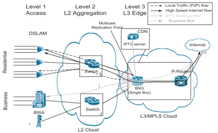
L2 Cloud L3/MPLS Cloud Internet DSLAM Switch P-Router IPTV server CDN Switch Multicast Replication Point Level 1 Access Level 2 L2 Aggregation Level 3 L3 Edge BNG (Single Box) J 1 ... BWA i Business Residential
Local Traffic (P2P) flow High Speed Internet flow
IPTV Multicast flow Business flow
Fig. 1. Centralized single edge overlay architecture.
BNG: Broadband Network Gateways are IP devices termi-nating the layer 2 access and route over IP/MPLS with support of a full set of MPLS and IP routing protocols, including multicast routing (PIM-SM/IGMP [8]). They enforce sophis-ticated IP QoS per service and per-content/source differenti-ation. They usually terminate PPP sessions or IP tunnels and can support up to hundred of thousands of subscribers and Gbps capacities. Edge routers, according to [1], can support additional functionalities related to Authentication, Authoriza-tion and Accounting (AAA) and are dynamic devices that mainly focus on residential customers. Moreover several next generation BNGs have the capability to support mobile blades to provide mobile termination functionalities.
MSE: Multi-Service Edge Routers are responsible for rout-ing business traffic, which is usually dedicated bandwidth. There is no need to authenticate the business users as these are leased lines, hence MSEs support less intelligence.
Video BNG: Video Broadband Network Gateways are dedicated routers that have been introduced to handle the increasing demand for video traffic (e.g. IPTV, Netflix etc.). A video BNG does not implement subscriber management functions (e.g., PPP termination, per user QoS), since these functions are likely to be performed by the other network elements. In fact the video BNG may be the point of insertion of an IPTV flow and/or the replication point (L3 Multicast).
B. Centralized Single-Edge Architecture
This type of design was very important in the early evo-lution of aggregation networks. In this type of architecture, the L2 Metro Ethernet aggregates the traffic from multiple access points and delivers the Virtual Local Area Network (VLAN) to the IP Edge network, as shown on Fig. 1. Some of the characteristics of this architecture are: 1) all types of traffic are backhauled to the BNGs and then to a single P-Router location, which is connected to the ISP backbone (P-Router is part of the backbone and sometimes called PoP); 2) Subscriber termination functionality, multicast replication and IP QoS policies are executed in the BNG deeper in the network; 3) Multicast traffic for broadcast video is transmitted from the edge router over L2 multicast VLANs to all customer premises (Wireless BS, DSLAM).
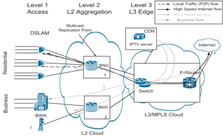
L2 Cloud L3/MPLS Cloud Business Wireless Internet Switch Residential P-Router IPTV server BWA
Switch Video Router
i BNG MSE J 1 ... CDN Multicast Replication Point Level 1 Access Level 2 L2 Aggregation Level 3 L3 Edge
Local Traffic (P2P) flow High Speed Internet flow
IPTV Multicast flow
Business flow
Fig. 2. Centralized multi edge overlay architecture.
C. Centralized Multi-Edge Architecture
In the multi-edge architecture there are different types of edge routers (BNG, Video BNG and MSE) that handle separate classes of subscriber and different types of traffic, as shown in Fig. 2. Residential subscribers are usually terminated in the BNG, whereas the Business VLANs or leased lines are routed through the MSE. Some providers, in order to enforce specific QoS policies on their video channels (IPTV), imple-ment a separate ’Video BNG’ [1]. Therefore, the Centralized Multi-Edge architecture benefits from incumbency, since it is easier to evolve from the existing architecture.
D. Distributed Single-Edge Design
A distributed IP Edge approach is being considered by many SPs as an alternative architecture to satisfy the bandwidth requirements for future applications. As shown in Fig. 3, the edge network is comprised by both L2/L3 routers. Video and HSI are backhauled over separate VLANs to the Edge Routers, where services and access to the IP network is controlled. The scalability is increased, since the amount of state information in the BNG is decreased (less subscribers are terminated per BNG) and IP QoS policies are enforced closer to the last mile. IP multicast routing is used across the L2/L3 Carrier Ethernet network for delivery of broadcast video services. In the single edge case, all services flow through a single device distributed closer to the subscriber.
Furthermore, based on the allocation of subscribers the aforementioned architectures can be further divided into:
• Clustered: Allocating the subscribers to a particular
ser-vice over many systems located in the same PoP.
• Unclustered: Allocating all subscribers for a particular
service to one system.
With the current centralized design, the increasing demand of video channels over IP networks leads to unavoidable bandwidth problem in the aggregation networks. Distributing the replication functionalities in multiple aggregation levels may result in less congestion of traffic bandwidth and VLANs, since a single unicast flow is required from the CDN to the distributed Video BNG. Moreover, the evolution of P2P IPTV sets new standards on how users interact. Distributing the IP intelligence can deal more effectively with traffic flows that
L2 Cloud L3/MPLS Cloud Internet P-Router IPTV server CDN Switch
Local Traffic (P2P) flow Multicast Replication Point Level 1 Access Level 2 L2 Aggregation Level 3
L3 Edge IPTV Multicast flowHigh Speed Internet flow
BNG Business flow J 1 ... BNG BWA i Business Residential DSLAM
Fig. 3. Distributed single edge overlay architecture.
tend to be “local”, since traffic is terminated and routed closer to the subscribers. In addition, several wireless providers are already facing issues on how to backhaul the increasing demand of mobile traffic. For this reason our work focuses on determining which architecture is the optimal one.
Finally, the distributed multi-edge architecture has been abandoned due to the increasing complexity of distributing multiple type of boxes over the aggregation network. Hence, we exclude it from the potential solutions.
IV. METHODOLOGY ANDASSUMPTIONS
A. Overview
The main objective of our work is to create a single modular and portable model that is able to provide the cost optimal solution among different architectural candidates. We model this through a mixed integer programming model. We divide the variables in qualitative (0-1) and quantitative. The quali-tative variables are used to select the appropriate architectural approach (Centralized vs Distributed), whereas the quantitative to determine the number of systems per location. The model is a non linear mixed integer; the non-linearity appears in the constraints. Such problems can be a challenging and daring venture, because they combine all difficulties of their subclasses: the combinatorial nature of integer programs (MIP) and the difficulty in solving non-convex nonlinear programs (NLP). Hence, we have transformed the problem to a linear one in the expense of extra constraints. In addition, we decreased the search space by defining upper bounds for the number of elements and interfaces. By using these heuristics the optimization problem was solvable in a finite amount of time.
In this model, we assume a tree topology (bipartite) with multiple aggregation levels. In fact, most of the ISPs usually implement small and medium aggregation sites and several core sites. The number of locations varies based on the size of the ISP. Small locations may vary from 10-10,000, the medium locations from 10-1,000 and the core location from 1-100. Every core site may support different kinds of areas (rural or non-rural) with various customer distributions. Thus, we are modeling a single three-level aggregation network. The results can then be extrapolated to include the whole ISP aggregation
TABLE I
MODELINGINPUTPARAMETERS
Description Symbol Ge ne ra l Access Location a= [1, ..., A] 1st Level Aggregation Locations i= [1, ..., I] 2nd Level Aggregation Locations j= [1, ..., J] Core Locations k= [1, ..., K]
Number of subscribers SUB
Subscribers per Residential Locationa resa
Subscribers per Business Locationa busa
DSLAM subscriber capacitya Sa
Number of IPTV Channels from CDN Ch
%of concurrent subscribers watching IPTV wi
Capacity of a Port c={1G,10G} A g g. S w itch Cost ($) co L2 Bandwidth (Gbps) CL2
VLAN capacity vlan
Number of slots for Ports PL2,c
Cost ($) of switching ports coL2,c
E
dge
Sys
tem
s Cost ($) for Typet coL3t
Bandwidth (Gbps) for Typet Ct
IP Termination Capacity for Typet subL3 t
Number of slots for Ports for Typet PtL3,c Cost ($) of routing ports coL3,c
infrastructure (multiple aggregation networks). In other words, solving the problem for the whole ISP network would require running the model multiple times for each aggregation network with different input parameters (e.g., subscribers, levels of aggregation).
B. Definitions
On the first level there may existAaccess locations. In each access locationa= [1, ..., A], the L2 access devices are able to handle a finite number of subscribers. On the remaining levels the model is going to define how to distribute the higher layer functionalities and how to handle different kinds of service flows.
1) Architecture: The first aggregation level is comprised
ofI locations (i= [1, ..., I]), the second level ofJ locations
(j = [1, ..., J]) and the last level of K = 1 single location
(single core site since we are modeling one aggregation area). The core site incorporates the P-Router which is responsible to route the non local traffic to the backbone or traffic from Tier-2/3 SPs (LAC/LNS functionality). However, it was not included as a variable in the model as it does not play any role on the functionality distribution. The insertion point of the video traffic from the CDN is assumed to be the core location. From the results, we noticed that if the insertion point was the Video BNG, the solution would have a very small variation.
2) Links: In order to model the links between each
aggre-gation level, we have used boolean constantsun−1,nfor every
aggregation level n ∈ {i, j, k}. If un−1,n = 1, then a lower
level locationn−1 is connected with a higher level location
n. However, it may be the case that the problem identifies that less aggregation levels are needed. Thus, in a similar manner
un−1,n+1 represents the connection with links between two
different layers.
3) Parameters: Table I summarizes the parameters of the
model. Our model is based on a network that has at most three aggregation levels. Our approach is able to determine, whether all three are needed or the ISP may decide to implement fewer
TABLE II
TYPES OFEDGEFUNCTIONALITIESt
Type Functionality Edge Design Combinations
A All Single Edge None
B HSI and Video Single/Multi Edge only type E C HSI and Business Single/Multi Edge only type F
D HSI Single/Multi Edge type E,F
E Business (MSE) Multi Edge type D,F or type B
F Video Multi Edge type D,E or type C
levels. In the same table, we also present the properties of each of the devices. Note that edge systems have the subscript t, which corresponds to different types. In regards to the port number, we make the following simplification: Edge system backplanes contain a finite amount of slots. In each slot, line cards are added that have a finite number of ports. Hence, instead of having so many variables, we have decided to associate the number of ports per device as the one to vary
PL3
t . Each port is also associated with a costcoL3,c.
4) Edge System Functionality: We also assume six different
types of edge routers t∈T ={A, B, C, D, E, F}, based on the functionality, the characteristics and the services that they support. We define the following edge system functionalities: • High Speed Internet (HSI): T1 = {A, B, C, D} ⊂ T
because they require IP termination;
• Business:T2={A, C, E} ⊂T for business subscribers; since they lease VLANs they do not require any termi-nation.
• Video replication (Multicast):T3={A, B, F} ⊂T. Table II summarizes the types, the functionalities, the edge design that they form, and the potential combinations with other edge systems at the same location. More specifically, in order to avoid redundancy of functionalities and therefore unnecessary cost, not all types of edge routers should be used in (a) a single location and (b) in any path from access node to P-router. For instance, if a BNG (type A) is used in a location
i, then it could perform everything in a single box, thus no other BNG should be installed in the same path (or location) towards the P-Router.
C. Variables
The objective function of the optimization problems is, given the appropriate locations, corresponding links and traffic demands, to optimally allocate the network elements and inter-faces, and identify where to place the routing functionalities. For this, there are two different types of variables, qualitative and quantitative1:
1) Qualitative Variables (0-1):
• uLn,t3 is a boolean variable that specifies which type of
system should be used at location n. If the edge router of type t is chosen at location n, then it is equal to 1; otherwise it is 0.
• uLn2 is a boolean variable that specifies if a switch is
going to be placed at location n or not. If it is, then it takes the value 1; otherwise it is 0.
1The variables are without an accent. Lower-caseuis used for qualitative
variables that take values 0 or 1, and upper-caseY is used for quantitative variables that are natural numbers
• u0n is a boolean that takes the value 1, if no device is
installed at all. That is uL3
n,t = 0,∀t ∈T and uLn2 = 0.
Evidently uL3
n,t+uLn2+u0n= 1.
• u1nG is a boolean variable that takes the value 1, if
1Ge interfaces (line cards) are chosen to be installed at location n; otherwise it is 0.
• u10nG is a boolean variable that takes the value 1, if
10Ge interfaces (line cards) are chosen to be installed at location n; otherwise it is 0.
Thus ifuL3
n,t = 0, then either a switch or another type of edge
system or nothing is installed. IfuL3
k,t= 1for any∀t∈T, then
the optimal architecture is the centralized one (according to the definition of the previous section). Whereas, if uL3
n,t = 1,
forn=k, the optimal architecture is the distributed. For the centralized case, if t=A, then the programming model will have selected the single-edge architecture.
2) Quantitative Variables: As quantitative variables we
define those variables that are natural numbers,N0. In this set there can be: ”real” variables, those associated with a specific characteristic and affect the objective function; ”dummy” variables, those that are used for other purposes and are not part of the objective function. The latter ones are used in the locations that the provider does not need to open or use. More specifically:
• Yn,nx,c,up+1 andY x,c,dn
n−1,n are the integer variables specifying
the number of interfaces of capacity c attached to the network element of layer x and located in location n. Those interfaces are attached to links that connect, either the uplink with one level higher (n+ 1), or the downlink with one level lower (n−1).
• Yn,tx is the integer variable specifying the number of
network elements x at location n and of type t. If
Yn,tL3 > 1 then it means that the location n needs its
routing functionalities to be clustered.
• Yn0 is the integer dummy variable that is used whenever
neither routing nor switching functionality is installed in location n. If all the n locations are in the same level have Yn0 >0, then this means that it is cost optimal to
have less aggregation levels.
• Yn,n0 +1,dn is the integer dummy variable that is used
to depict a fictional number of interfaces, whenever no device is determined to have been installed at then+ 1
location,Yn0+1= 0.
V. MODELING THETRAFFICFLOWS
In our modeling approach, we assume that the beginning of the traffic is the first aggregation point, or else any access location a. This was done for several reasons: a) the number of subscribers may range to millions, making the problem hard to be solved with that amount of variables and constants; b) network architects usually use mean (or some percentage) traffic demands over subscribers of a bigger geographical area [3], [18]; c) according to the VLAN policy implemented, traffic subscriber VLANs are bundled into a bigger VLAN per service from the access location (e.g. DLSAM in wired and nodeB in 4G wireless) until the edge location (BNG in ethernet aggregation or RNC in 4G wireless); d) the service providers do not tend to incorporate L3 type capabilities and
TABLE III
VOLUMES OF TRAFFIC
Traffic Volume per subscriber
HSI traffic (Mbps) for residential customers HSIres a
HSI traffic (Mbps) for business customers HSIabus Bidirectional P2P (Local traffic) in Mbps P2Pa
IPTV Bandwidth (Mbps) of each channelch iptvch Internet (Non local Traffic) flowing
through the locationn xHSI n
IPTV Traffic flowing
through the locationn xIP T V n
from the CDN to the first IP replication point xCDN n
P2P (Local Traffic) flowing
through the locationn xP2P n
from one level below xP2P n,dn,in
from one level above xP2P n,up,in
to one level below xP2P n,dn,out
to one level above xPn,up,out2P
management functionalities that close to the subscribers. For example HSIares (on table III is calculated by taking into
account the harmonic mean of the bandwidth consumed per subscriber that is served by the access location a. However, an ISP may properly configure the per subscriber usage in order to assume a worst case (or some percentile) and possibly overprovision the network [19]. In the evaluation, we are investigating a variety of network throughput and showcase the effect of the traffic demand into the optimal solution.
The traffic classes and service types are generally available to the ISPs, since BNGs incorporate DPI or flow classification functionalities [6]. For modeling reasons, we have grouped the traffic flows into three main classes, i.e. IPTV, Internet (Non Local) and P2P (Local). The traffic demands are shown on Table III.
We categorize the traffic flows according to the effect (utilization, direction etc.) that they have on each aggregation leveln∈ {i, j, k}. Hence we define three main categories of traffic class:
A. Internet (non local) Traffic Class
Internet traffic class is any type of residential or business traffic that will flow through all the levels of the aggregation network. It is usually a client-server type of traffic and its major portion is usually web traffic [18]. In terms of network optimization, this type of traffic satisfies the conservation theorem, unless redundancy elimination devices are included in any level of the network [23]. The Internet traffic per aggregation level is represented by the following equations.
xHSIi =
a
ua,i(xresa +xbusa )
xHSIj = i ui,jx HSI i (1) xHSIk = a (xresa +x bus a )
The non local traffic that flows through an access locationa
is based on the number of subscribers and the corresponding network usage per subscriber. Thusxres
a =resa·HSIaresand
xbus
a =busa·HSIabus, indicate the bundled traffic that arrives
in an access location, for residential and business subscribers respectively. The reason that we use separate volumes for each
type of subscriber is because the network usage is different and their connections towards the “edge systems” are different.
B. P2P (Local) Traffic Class
P2P traffic class includes those applications that exhibit locality in their behavior. Those traffic flows are distributed across the aggregation network over several directions and may either remain local in the same geographical area (e.g., P2P or a business unit that has a local server), or in the same routing domain, and depend on how peers are interconnected. In P2P systems the files are split in smaller chunks and are downloaded from various sources. The system is therefore initiating various flows to various users. The P2P flow will have different performance based on the placement of the routing functionalities. Let us assume that users in the same access location are downloading P2P traffic with a certain throughput P2Pa Mbps from sources that are either in the
same edge network or outside the aggregation area. Therefore, the total P2P traffic that flows through an access location is
xPa2P =subaP2Pa.
The distribution of functionalities is also affected by the overlay P2P network. If the user is downloading a file from peers in the same first aggregation level then we denote this probability with p1. Similarly if the two peers coexist at the same second aggregation level location, their probability isp2, andp3 for the third aggregation level location. Since the P2P files are usually divided in chunks, the above probabilities can be regarded as equal to the portion of traffic that is coming from users at the same aggregation level. Practically those probabilities are related to the direction of the traffic, and can be calculated by the ISP through performing flow identification (such functionality can be found in both L2/L3 devices). Equivalently for the flow that goes outside of the network1−3l=1pl. The question now is how this probability
may affect the cost of the architecture.
The following equations show how the P2P traffic flows over the networks. Effectively the first equations bundles the P2P traffic into a VLAN that will be offered to the first aggregation layer i. The existence of a router of type t at any level k, as defined by the variable uL3
k,t will affect the
direction of the flow. For example, if a router that performs IP termination (t∈T1) is placed at the first aggregation layer (uL3
i,t = 1), all traffic that would remain local at the first
aggregation layer would not have to flow through the rest of the layers. Similarly for the rest of layers
xPi 2P = a ua,ix P2P a xPj2P = t∈T1 [uLk,t3xPk2P+ i ui,jxPi2P(uLj,t3+uLi,t3 3 k=2 pk)] (2) xPk2P ={(1− t∈T1 uLk,t3)(1− 2 k=1 pk) + t∈T1 uLk,t3} j xPj2P
C. Multicast Traffic Class
Multicast is required in order to make efficient use of net-work resources when delivering broadcast content. Mainly, the desired goal is to support multicast optimization by controlling
the flooding of Ethernet multicast frames. The IGMP/PIM-SM agents can locally adjust replication filters on the device, such that packets are replicated only on those ports that have specifically requested to be part of the multicast group [8]. However, the location of the multicast functionality (either as IGMP snooping on L2 devices, or as IP multicast on L3 devices) is based on the VLAN architecture. In the following, we assume that the VLAN policy implemented by the ISP requires the replication to happen in the edge system.
A unicast IPTV traffic flow is assumed to be initiated from the CDN(s) and is replicated at the Edge Router, where multicast is implemented. The streaming bit rate is usually between iptvSD
ch =1Mbps for Standard Definition (SD) and
iptvHD
ch =10Mbps for HD channels and the user is assumed
to choose either the channel in one definition or in the other [30]. Several studies have shown that the selection of IPTV channels ch ∈ {1, ..., Ch}, follows a Zipf Law distribution
pch=α/ch, given that the channels are arranged by channel
popularity [31] (αis a constant). It is also assumed that the percentage of residential users per a access locations (e.g., DSLAM, Wireless Base station) that have selected the IPTV service is wa.
In order to calculate the required bandwidth for the unicast transmission of IPTV channels, from the CDN to the first replication point, the number of requested channels, from the residential subscriber population, needs to be determined. The probability that at least one user is watching a channel c, and belongs at the subtree formed by the location n, can be determined as 1 − P{none watching channel ch}(t) =
1−(1−pch)
awa·resa·ua,n
. Therefore, regarding the unicast flow from the CDN to the first IP replication point, the bandwidth can be defined by the following equation
xCDNn =iptv HD ch +iptv SD ch 2 · Ch c=1 1−(1−pc) awa·resa·ua,n (3) After the flow reaches the Video router all flows are distributed to the subscribers through multicast. However, the distribution of video routing functionality plays a role on the distribution of IPTV flows over the network. Note that if a multicast routing functionality has been determined to exist in that location, then the flow conservation theorem does not hold (since the video router will replicate the IPTV flow to the corresponding IPTV VLANs). For example, if a single BNG is placed in the first aggregation level, then the multi-cast is going to happen closer to the subscribers. Therefore the IPTV flow that every access location is demanding is
xIP T V
a =wa·resa·IP T Vch (percentage of userswa from
the population of suba connected to access locationa), then
the flows are going to be distributed in the network as follows
xIP T Vi = a ua,ix IP T V a xIP T Vj = i ui,j[ t∈T3 uLi,t3x CDN j + (1− t∈T3 uLi,t3)x IP T V i ] (4) xIP T Vk = a xIP T Va t∈T3 uLk,t3+x CDN k (1− t∈T3 uLk,t3)
For the first definition of the above equation,xIP T V
i is equal
to the bandwidth that all IPTV VLANs generate. For the
xIP T V
j , there are two possibilities. If a typeT3router is placed
at any of the dependent first aggregation levels (uLi,t3 = 1),
then the bandwidth of the IPTV flows is equal toixIP T V
i .
If this is not the case, then the bandwidth is equal to the eq. (1). The third equation takes into account the property
t∈T3(u L3
i,t +uLj,t3 +uLk,t3). Thus, if a router that includes
IPTV functionality is included at the central location k, then the IPTV bandwidth is axIP T V
a . Otherwise it means that
an IPTV capable router has been placed in either the 1st or the 2nd aggregation level and the bandwidth for the flow is
xCDN
k
iptvHDch +iptvchSD
2 . From the above, it is readily seen that if users tend to watch similar programs, less bandwidth is used, decreasing the infrastructure cost. In addition, integrating the multicast functionality (i.e. t ∈ T3), closer to the access network, decreases the bandwidth too.
Therefore the total amount of traffic that arrives in every aggregation location isxn=xIP T Vn +xnP2P+xHSIn .
VI. EDGEDESIGNMODEL
The objective function of the optimization problem is to determine the optimum deployment cost by optimally dis-tributing the functionalities over the aggregation network
min n∈{i,j,k} [ c x (cox,cYnx,c) + t coLt3Y x n,t+co L2 YnL2] (5) The above objective function includes the cost of the interfaces based on the capacityc= [1G,10G], that will be implemented in a node of layerx= [L2, L3]at locationn, as well as the cost of the network elements that will be placed at the same location.
A. Constraints
1) Non Linear to Linear Transformation: The problem has
two sets of variables per location,YL3
n,t anduLn,t3. The
multi-plication of those variables results in a non linear problem. Hence, we try to transform the model from a non-linear to a linear, by adding some extra constraints along with two big constants BIGDn (for the devices) and BIGIn (for
the interfaces). For example, devices per location may range between 10-100, therefore BIGDn can be as high as 1000.
Any value higher than that may result in an unnecessary increase of the search space. In the next section, we provide a heuristic to determine an approximate upper bound. The extra constraints are expressed as follows:
Yn,tL3≤BIGDn YnL2≤BIGDn(1− t∈T1 uLn,t3), n∈ {i, j, k} (6) {t∈T1|n=i, j}or {t∈T|n=k} The above constraints specify that (a) the YL3
n,t must be
bigger than a big constant, and (b) in every locationn there can be only an aggregation switch or an edge system. In terms of functionalities, the two sets define that for the first and second aggregation levels n = {i, j}, only IP termination functionalities can be distributed (t∈T1). The last set effec-tively excludes the multi-edge architecture from the possible
solutions. We follow a similar approach for the interfaces. YnL3,c≤BIGIn t∈T1 uLn,t3, {t∈T1|n=i, j},{t∈T|n=k} YnL2,c≤BIGIn(1− t∈T1 uLn,t3),n∈ {i, j, k} (7) YnL3,c+Y L2,c n ≤BIGInucn,n∈ {i, j, k}
The first constraint, of the above set, defines that an edge system interface will be chosen if at least one edge system is installed in that location. The second constraint shows that an aggregation switch at location n must not be installed if an edge router is installed at this location. The last constraint indicates that either a 1Ge or 10Ge interface can be installed at a network device.
2) Avoiding redundancy of functionality: In order to avoid
the redundancy of functionality in a path, only a certain combination of routers can be used per path. The path starts from the access node and ends at the P-Router, and can be represented by the multiplication of the following binary constants ui,juj,k. In that path, each functionality must not
be repeated (which is represented by the sum of the binary variables in the path must not be greater than one) and certain functionality must not be used.
ui,juj,k t∈T1 uLi,t3+u L3 j,t +u L3 k,t≤1 ui,juj,k( t={A,C} (uLi,t3+u L3 j,t) + t∈T2 uLk,t3)≤1 ui,juj,k( t={A,B} (uLi,t3+u L3 j,t) + t∈T3 uLk,t3)≤1 ui,juj,k≤ t∈T1 uLi,t3+u L3 j,t+u L3 k,t (8) ui,juj,k≤ t={A,C} (uLi,t3+u L3 j,t) + t∈T2 uLk,t3 ui,juj,k≤ t={A,B} (uLi,t3+u L3 j,t) + t∈T3 uLk,t3
3) Capacity Constraints: The capacity constraints define
the amount of traffic that either an aggregation switch or an edge system can support. This is effectively the backplane capacity. For the case of a distributed routeruLn,t3 = 1selected
at location n = {i, j}, the following two constraints are defined uLn,t3(x CDN n +x res n +x bus n +x P2P n )≤Y L3 n,tC L3 t , (9) ∀n={i, j}, t={A, B} uLn,t3(xIP T Vn +xresn +xbusn +xPn2P)≤Yn,tL3CtL3, (10) ∀n={i, j}, t={C, D}
Type A and B do have multicast functionality, therefore they will replicate the traffic. Hence, only the flows that correspond to the requested channels need to be routedxCDN
n .
Nonetheless, if type C or D are selected to be distributed, then the replication of the channels is done in the core location, and they will need to route the bundled flows for the multicast traffic. Starting from the top, type A router handles all traffic, therefore the throughput at a central k must be less than the
total throughput of the routers of type A. Note that type A handles all types of traffic, thus it serves all the traffic
xCDN
k +xbusk +xresk +xPk2P. Similarly for the rest, with the
main difference that only a subset of functionality are support per edge system.
uLk,A3(x CDN k +x bus k +x res k +x P2P k )≤Y L3 k,ACA uLk,B3 (x bus k +x res k +x P2P k )≤Y L3 k,BCB uLk,C3 (x res k +x bus k +x P2P k )≤Y L3 k,CCC uLk,D3 (x res k +x P2P k )≤Y L3 k,DCD (11) uLk,E3 x bus k ≤Y L3 k,ECE uLk,F3 xCDNk ≤Yk,FL3CF
For the switching capacity things are more complicated as the capacity is affected by the distribution of the edge system functionality. For example, the closer the multicast functionality is to the subscribers, the closest the replication takes place. Equation (VI-A3) indicates the switching capacity constraints. The first is related to the locations in the first aggregation level i. This constraint indicates that if an edge system is installed uL3
i,t = 1 then there is no need to care
about the switching capacity. The second constraint is related to the locations in the second aggregation levelj. If multicast replication takes place at lower level uL3
i,A+uLi,B3 = 1, then
only a single flow per channel needs to be switched xCDN.
If it is taking place at the core location, uLi,C3 +u L3
i,D = 1
or t∈T
3u
L3
k,t = 1(T3 is the set of the routers that support
multicast), then a separate flow per subscriber for the IPTV needs to be switched. Finally, if a router is placed at the second aggregation level uL3
j,t = 1, then there is no need to
switch any traffic. If a switch is placed in a core location and also an MSE or Video BNG is placed at the same location, then they will route business and IPTV traffic and therefore those two portions need to be excluded from the switching capacityxbus k (1− t∈T2uLk,t3)+xCDNk (1− t∈T3uLk,t3). Those
constraints can be found in the inequality set (VI-A3) at the top of the next page.
4) Subscriber Termination/VLAN Capacity: The following
equalities determine the number of VLANs per location. A distinction is made between the residential and the business VLANs. Sires= a ua,iS res a , S bus i = a ua,iS bus a Sresj = i ui,j(1− t∈T1 uLi,t3)S res i Sjbus= i ui,j(1− t={A,C} uLi,t3)S bus i (13) Sresk = j (1− T1 uLj,t3)S res j Skbus= j (1− t={A,C} uLj,t3)S bus j
For routers of type A, B, C and D which may exist at any of the levels n = {i, j, k} the subscriber termination constants are similar to the capacity ones. They are expressed as followuL3
n,tSn ≤Yn,tL3, whereSn =Sresn +Snbus for Type
(1− t∈T1 uLi,t3)(x IP T V i +x res i +x bus i +x P2P i )≤Y L2 i Cags i (ui,j(uLi,A3 +u L3 i,B)x CDN k + (u L3 i,C+u L3 i,D)x IP T V i ) + t∈T3 uLk,t3x IP T V j + (x res j +x bus j +x P2P j )(1− t∈T1 uLj,t3)≤Y L2 j Cags (12) (1− t∈T1 uLk,t3)(x CDN k +x res k +x bus k +x P2P k ) +x bus k (1− t∈T2 uLk,t3) +x CDN k (1− t∈T3 uLk,t3)≤Y L2 k Cags and Sn =
awaRESa for Type F. The latter is expressed
lie that as all these must be terminated at the Video BNG, because only a portion wa of subscribers are watching a
channel and the total number of IPTV VLANs are determined by awaresa
For VLANs that need to be switched, the case is a bit more complicated. For the second level of aggregation and if a cus-tomer has been already been terminated in the previous level, thenJ−1VLANs will be required to switch traffic among the same level of switches and one more that will send the traffic to the P-router. If however only the residential subscribers have been terminated in the previous level (uL3
i,B+u
L3 i,D= 1)
then the business VLANs will still remain (Sbus
i +J). The
constraints for the VLAN capacity are mentioned in the next page, inequality (14)
5) Link and Interface Constraints: Each access location
is assumed to have Na devices and each location has both
uplink and downlink interfaces. The minimum number of downlink interfaces from the first aggregation level is equal to the number of access devices that are connected to this location, i.e. ua,iNa. In every of the first and second level
aggregation locations either a router or a switch or nothing is placed. Therefore, two of the YnL−3,c,dn1,n , Y
L2,c,dn
n−1,n andY0
,dn i,j
are going to be zero.
ua,iNa≤ c (Ya,iL3,c,dn+Y L2,c,dn a,i ) ui,j( t∈T1 Yi,tL3+Y L2 i )≤Y0 ,dn i,j + c Yi,jL3,c,dn+Y L2,c,dn i,j t∈T1 Yj,tL3+Y L2 j + i Yi,j0,dn≤ c Yj,kL3,c,dn+Y L2,c,dn j,k (15)
The network elements also have line card capacity. Each line card is a separate module that has a specific capacity of ports and functionalities. We assume two types of line cards, one for switches and one for routers. Each element may take ports of the same type, 1Ge and 10Ge, and the port capacity is determined by multiplying the number of line card slots to the number of ports per line card. Since the number of ports per line card is affected by the bandwidth of the interfaces, the same will hold for the total number of ports per network
element. The constraints are expressed as follows.
a ua,iY L2,c,dn a,i + j ui,jY L2,c,up i,j ≤Y L2 i P L2,c i a ua,iY L3,c,dn a,i + j ui,jY L3,c,up i,j ≤ t∈T1 Yi,tL3P L3,c i,t i ui,jY L2,c,dn i,j +Y L2,c,up k ≤Y L2 j P L2,c j (16) i ui,jY L2,c,dn i,j +Y L2,c,up k ≤ t∈T Yj,tL3P L3,c i,t
As we can see above, the first constraint makes sure that there is at least one link between the access node and the first aggregation level. However if the solution determines that no device is going to be installed, thend→ ∞andYi0= 1.
6) Interface Capacity Constraints: The interface capacity
constraints are the most complicated, since they must be determined without any knowledge of the placement of the devices. In every device there are going to be interfaces that connect both the uplink and the downlink.
Ynx,c=Y
x,c,dn n−1,n +Y
x,c,up
n,n+1 (17)
gives the total number of interfaces of capacitycper location
n. Moreover, in all cases the uplink capacity is equal to the downlink capacity of the higher layer. For instance for the link between the access locationaand first, the constraint is as fol-lowsua,i(xIP T Va +xresa +xbusa +xPa2P)≤
c xY x,c,dn a,i C c . For the links betweeniandj, The bandwidth of the uplink of the first aggregation level is calculated to be: a) the internet and business traffic (non local flows); b) if a multicast functionality is placed at the first level, uL3
i,A+uLi,B3 = 1, the flow of the
channels from the second aggregation levelxCDN
j ; c) if there
is not a multicast functionality1−t∈T
1u
L3
i,t = 1on the first
level, the IPTV flow of each subscriber; d) if there is routing functionalityt∈T
1u
L3
i,t = 1 the P2P portion that is not first
level local(1−p1)xP2P
i . For simplicity we mention only the
downlink constraints (the uplinkitojare the same). Similarly the remaining interface capacity constraints are calculated for the other two aggregation levels.
VII. MODELIMPLEMENTATION
As a mixed integer programming model, the problem is considered to be NP-hard (polynomial time hard). We applied two heuristics to decrease the number of variables. After this phase, we used the branch-cut-algorithm from the CPLEX 11 engine. Finally, we used the CPLEX presolver to eliminate redundant rows and columns. In the following we describe the two heuristics:
(1−
t∈T1
uLi,t3)Si≤YiL2subags
i ui.j((u L3 i,A+u L3 i,C)J+ (u L3 i,B+u L3 i,D)(S bus i +J)) + t∈T1 uLk,t3Sk≤YiL2subags (14) ui,j((u L3 i,A+u L3 i,B)x CDN j + t∈T1 uLi,t3(1−p1)x P2P i + (1− t∈T1 uLi,t3)x IP T V i +x P2P i ) +x HSI i +x BU S i ≤ c x Yi,jx,c,dnC c (18) xHSIj +x BU S j + (1− t∈T1 uLj,t3)(1−p1−p2)x P2P j + (1− t∈T3 uLj,t3)x CDN k + t∈T3 uLj,t3x IP T V j ≤ c x Yi,kx,c,dnC c (19) xHSIk + (1− 3 k=1 pk)xPk2P +x CDN k +x BU S k ≤ c x Ykx,c,upC c (20) TABLE IV
INPUTPARAMETERS FORAGGREGATIONNETWORKCHARACTERISTICS
ANDINTERFACEPROPERTIES
Symbol Descr/Units Small SP Big SP
A Locations 1000 2000 I Locations 6 50 J Locations 3 5 K Locations 1 SUB Subscribers 200K 400K resa Subscribers 160K (80%) 320K (80%) busa Subscribers 40K (20%) 80K (20%) Sa Subscribers 200 Ch Channels 100 wi %of viewers 50% CL2 1G/C10L2G Bytes 1G/10G CL3 1G/C10L3G Bytes 1G/10G coL2,1G $ 1K coL3,1G $ 2K coL2,10G $ 2K coL3,10G $ 4K
Heuristic 1: Minimizing number of variables.Generally the number of access locations A varies from hundreds to thousands making the problem hard to be solved. For this, we implemented a clustering algorithm to determine the number of access locations. The algorithm starts with a single cluster
cl= 1, increases the number of clusters in every iteration, and terminates when both the time to convergence is smaller than a predefined valuetand the optimality tolerance is also smaller than a predefined value ac. This means that the number of access locations will be A=cl∗I, whereclis the number of clusters. The divisive clustering procedure is as follows
1: procedureCLUSTER(I, t, ac)
2: cl←1
3: A←I
4: Run model to determinetandac
5: while t≤t andac≤ac do
6: cl←cl+ 1
7: Perform K-means clustering
8: A←cl∗I
9: Run model to determinet andac
10: end while 11: return cl
12: end procedure
In every iteration, the K-means instance [16] is called
with attributes related to the technical characteristics of the access devices. In our case we used as attributesthe L2 subscriber capacity of the access technologies. After running the optimization model several times, we determined that if the model does not converge to a solution in less thant= 120sec
, it will hardly manage to converge (soft threshold). Finally the optimality tolerance was set to10−6. In any case, a potential error in terms of Kbps will not affect the solution of the model (since all system capacities are at the order of thousands of Gbps).
Each access location is assumed to incorporate the same access device. However, the definition of the “location” in our model is not strictly a geographical location. Therefore, if in the same geographic location different access technologies are implemented, then these are treated as two separate locations.
Heuristic 2: Minimizing execution time.The optimization has integer variables that are either binary (qualitative) or non-binary (quantitative). In order to transform the problem to integer programming model, the values of BIGIc
n and
BIGDn were introduced. If these values are selected to be
very big, then the solver would require a significant amount of time to converge to an optimal solution. If the values are selected to be small, the solution would not be the optimal (or the problem could be infeasible). Thus the values were selected by taking into account the amount of traffic that flows and the number of VLANs in the corresponding location. A logical upper bound for the number of devices per aggregation location can be derived from
BIGDn=max{ X n min{CL3 t , t∈T} , subn min{subL3 t , t∈T} } (21) For an upper bound on the number of interfaces, we used the above upper bound multiplied by the most numbers of ports
BIGInc =BIGDn∗max{Ptc,L3, t∈T},c∈ {1G,10G}
(22) Using the above values the solver was determining the solution in less than 1min on an Intel Core2 Duo T7700 with 4GB RAM.
VIII. EVALUATION ANDRESULTS
In this section, we use two exemplar architectures to evaluate the aforementioned edge design model. The first
TABLE V
NETWORKELEMENTFEATURES
Edge Cost Capacity IP Term. 1Ge 10Ge
System coL3,t(K$) Ct(Gbps) subL3, t PL1G3,t PL103G,t All 300 160 64000 192 24 HSI/VideoBNG 600 640 64000 480 64 HSI/MSE 220 40 32000 96 12 HSI 340 280 32000 140 28 MSE 180 20 4000 96 12 Video BNG 200 280 10000 140 28
Cost Switching VLAN 1Ge 10Ge
K$ Ct(Gbps) vlan PL1G2 PL102G
Agg. switch 270 280 64000 140 28
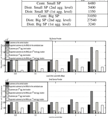
architecture, namely ”small SP”, is based on an EU ISP with 200K subscribers. The second architecture, namely ”big SP” is based on another EU ISP with twice the number of subscribers, and ten times more first level aggregation locations. We use several traffic scenarios per subscriber (very low up to very high). We performed this investigation such that a future traffic growth is incorporated in our modeling. In table IV, the details of the architectures are given. In table V the values for each edge system are showcased. These values were provided by vendor and are representative of high-end systems at the time of submission2. The number of interfaces in the table is derived by multiplying the number of ports per line card with the capacity of line cards per edge system. In addition the local (P2P) traffic does not exceed 20% of the total internet traffic [18] and P2P locality probabilitiespk get
values from a uniform distribution. The questions that we try to address are as follows
• Which of the functionalities should the provider distribute closer to the subscriber?
• Does the size of the ISP affect the choice of the optimal functionality placement?
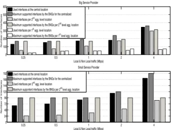
• Should the providers choose faster (but more costly) line cards or a faster backplane in an Edge Router?
• What is the usage (or how much redundancy exists) per edge system for throughput, termination capabilities and port availability?
• How does a change in the number of subscribers affect the intelligence distribution?
In Fig. 4 the cost of multiple architectures is shown for the big service provider. The centralized and 2nd level distributed architectures are investigated. The 1st level aggregation is the first level above the access network and similarly for the rest. Due to the number of 1st level aggregation locations, we found that the cost of distributing the functionalities at the 1st level was higher than in the other two. For this reason, the centralized and the 2nd level distributed architectures were chosen to be plotted. In the case of a small amount of multicast flows, the centralized unclustered seems to be the cost optimal architecture. This is because most of the traffic goes through the central locations to the backbone. However, an increase of multicast traffic leads to significant increase in the cost of the
2The prices of those systems may vary over time and offer. However
those values are representative at the time of submission through private communication with at least one vendor. An incremental change of those values does not affect the formulation of the problem.
0 2 4 6 8 10 3.4 3.6 3.8 4 4.2 4.4 4.6 4.8 5 5.2x 10 4 IPTV Mulicast (Mbps) Cost (K$) 0.5Mbps Internet Traffc 0 2 4 6 8 10 6.5 6.6 6.7 6.8 6.9 7 7.1 7.2 7.3 7.4 7.5 7.6x 10 4 IPTV Multicast (Mbps) Cost (K$) 4Mbps Internet Traffic Centralized Unclustered Centralized Clustered (BNG/MSE) Distributed Unclustered (2nd agg. level)
Distributed Clustered (2nd agg. level for BNG)
Centralized Unclustered Centralized Clustered (BNG/MSE) Distributed Unclustered (2nd agg. level) Distributed Clustered (2nd agg. level for BNG)
Fig. 4. Cost comparison for the big service provider per aggregation network for 0.5Mbps and 4Mbps of local and non local traffic (Internet).
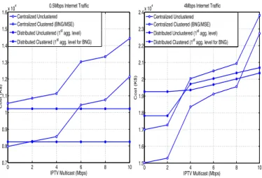
0 2 4 6 8 10 0.7 0.8 0.9 1 1.1 1.2 1.3 1.4 1.5 1.6x 10 4 IPTV Multicast (Mbps) Cost (K$) 0.5Mbps Internet Traffic 0 2 4 6 8 10 1.5 1.6 1.7 1.8 1.9 2 2.1 2.2 2.3 2.4x 10 4 IPTV Multicast (Mbps) Cost (K$) 4Mbps Internet Traffic Centralized Unclustered
Centralized Clustered (BNG/MSE) Distributed Unclustered (1st agg. level)
Distributed Clustered (1st agg. level for BNG)
Centralized Unclustered Centralized Clustered (BNG/MSE) Distributed Unclustered (1st agg. level) Distributed Clustered (1st agg. level for BNG)
Fig. 5. Cost comparison for the small service provider per aggregation network for 0.5Mbps and 4Mbps of local and non local traffic (Internet).
centralized architecture.
On the other hand, the rate of cost increase for the dis-tributed is smaller, and after some point it becomes cheaper. The point at which the graphs meet is important. It effectively shows at which point the SP will need to distribute the functionalities. For small amounts of internet traffic (0.5Mbps per user) the meeting point is around 8 Mbps of multicast traffic, and for a much larger internet traffic (4Mbps per user) it is around 4Mbps. In such large amounts of traffic, either the capacity constraints of the elements or the port constraints are met, leading to more devices/interfaces. Therefore, the distribution of IP intelligence is preferable, because (a) it alleviates the bottleneck due to P2P traffic that in any other case would need to go the central location and (b) the
multicast traffic is replicated closer to the access network.
Finally, clustering the devices does not have a positive impact (compared to the unclustered case) to the cost. In the Big SP there is enough ”capacity” (by ”capacity” here we mean the shadow price of the subscriber, traffic and port constraints) to support all different services.