Weighting in survey analysis under informative sampling

(1)

Statistics Publications Statistics

2013

Weighting in survey analysis under informative

sampling

Jae Kwang Kim

Iowa State University, jkim@iastate.edu

C. J. Skinner

London School of Economics and Political Science

Follow this and additional works at:http://lib.dr.iastate.edu/stat_las_pubs

Part of theDesign of Experiments and Sample Surveys Commons, and theStatistical Methodology Commons

The complete bibliographic information for this item can be found athttp://lib.dr.iastate.edu/ stat_las_pubs/109. For information on how to cite this item, please visithttp://lib.dr.iastate.edu/ howtocite.html.

This Article is brought to you for free and open access by the Statistics at Iowa State University Digital Repository. It has been accepted for inclusion in Statistics Publications by an authorized administrator of Iowa State University Digital Repository. For more information, please contact

(2)

Jae Kwang Kim and

Chris J. Skinner

Weighting in survey analysis under

informative sampling

Article (Accepted version)

(Refereed)

Original citation:

Kim, Jae Kwang and Skinner, Chris J. (2013) Weighting in survey analysis under informative sampling. Biometrika, 100 (2). pp. 385-398. ISSN 0006-3444

This version available at: http://eprints.lse.ac.uk/50505/

Available in LSE Research Online: August 2014

LSE has developed LSE Research Online so that users may access research output of the School. Copyright © and Moral Rights for the papers on this site are retained by the individual authors and/or other copyright owners. Users may download and/or print one copy of any article(s) in LSE Research Online to facilitate their private study or for non-commercial research. You may not engage in further distribution of the material or use it for any profit-making activities or any commercial gain. You may freely distribute the URL (http://eprints.lse.ac.uk) of the LSE Research Online website.

This document is the author’s final accepted version of the journal article. There may be differences between this version and the published version. You are advised to consult the publisher’s version if you wish to cite from it.

(3)

Weighting in survey analysis under informative

sampling

Jae Kwang Kim

Department of Statistics

Iowa State University

Ames, Iowa 50011, U.S.A.

Chris Skinner

Department of Statistics

London School of Economics and Political Science

London, WC2A 2AE, U.K.

May 14, 2013

Abstract

Sampling related to the outcome variable of a regression analysis conditional on covariates is called informative sampling and may lead to bias in ordinary least squares estimation. Weighting by the recipro-cal of the inclusion probability approximately removes such bias but may inflate variance. This paper investigates two ways of modifying such weights to improve efficiency while retaining consistency. One approach is to multiply the inverse probability weights by functions of the covariates. The second is to smooth the weights given values of the outcome variable and covariates. Optimal ways of constructing weights by these two approaches are explored. Both approaches re-quire the fitting of auxiliary weight models. The asymptotic properties of the resulting estimators are investigated and linearisation variance estimators are obtained. The approach is extended to pseudo maxi-mum likelihood estimation for generalized linear models. The prop-erties of the different weighted estimators are compared in a limited simulation study. The robustness of the estimators to misspecification

(4)

of the auxiliary weight model or of the regression model of interest is discussed.

Keywords: Complex sampling, Pseudo maximum likelihood estimation, Regression analysis, Sample likelihood.

1 Introduction

Survey data are often used to make inference about superpopulation models from which finite populations are assumed to be generated. When survey data are obtained from units selected with complex sample designs, the re-sulting analyses require different methods to those developed classically un-der random sampling assumptions. [?], [?] and [?] provide overviews of this topic. Regression is a key tool for statistical analyses that describe the struc-tural relationship between survey variables. Survey weights are often used in regression analysis of survey data to ensure consistent estimation of pa-rameters when sampling may be informative, that is when sample inclusion may be related to the outcome variable conditional on covariates [6.3]fuller09. Although weighting has this bias-correction advantage, it also brings the dis-advantage of often leading to a loss of efficiency relative to an unweighted approach.

A number of authors have considered how the survey weights may be modified to improve efficiency while retaining their advantage of ensuring consistency under informative sampling. [?] showed that consistency is re-tained under any multiplication of the weights by a function of covariates and suggested how such a function might be chosen. [?] proposed a modification of the weights by a function of the covariates which minimized a prediction

(5)

criterion. [?] discussed both approaches and extended their consideration of variance estimation. [?] extended their approach to generalized linear mod-els. [6.3.2]fuller09 showed how efficiency could be maximized for a class of modified weights. [?] extended Fuller’s approach in the context of a cross-national application. Addressing a rather different inferential problem, [?] proposed smoothing survey weights, with a modification which depends on the survey variables, in order to improve efficiency of descriptive estimation. In this paper, we show how the ideas of [?] and [?] may be integrated in the regression analysis of survey data by considering a weight modification which is a function of both the outcome variable and covariates and we develop and evaluate associated inferential methods, including variance estimation.

Alternative approaches, especially likelihood-based methods, have also been proposed for efficient inference about regression parameters in the pres-ence of informative sampling. See [?], [?], [?] and [?] and references therein. However, in this paper we restrict attention to weighting methods, which are widely used in survey practice and for which various weight modifications are already familiar to survey data users.

2 Basic set-up

We consider the regression of a variable y on a vector of variables x. Let (x0_i, yi) denote the row vector of values of these variables for a unit with label

iin the index setU ={1, . . . , N}of a finite population of sizeN and suppose that these values follow the regression model

(6)

whereE(ei |xi) = 0. We assume a probability sampling design, where

inclu-sion in the sample is represented by the indicator variables Ii(i= 1, . . . , N),

where Ii = 1 if unit i is included in the sample and Ii = 0 otherwise and

πi = (Ii = 1 |i) is the first-order inclusion probability. Then the ordinary

least squares estimator of β0 solves

N

X

i=1

Ii(yi−x0iβ)xi = 0 (2)

for β, and this estimator will generally be biased unless sampling is non-informative, that is Ii and yi are pairwise independent conditional on xi,

(Ii = 1|yi, xi) = (Ii = 1|xi). (3)

In some circumstances it is possible to ensure that sampling is non-informative by including in xi all of the design variables which explain

vari-ation in the πi. Many surveys, however, exhibit variation in the πi which,

at least in part, is attributable to practical features of the survey imple-mentation and cannot be wholly explained by variables which would be of scientific interest as covariates in the model. Thus, it is more realistic to write πi =πi(X, Z) as a function of the population values X = (x1, . . . , xN)

and Z = (z1, . . . , zN) of both xi and a vector of design variables zi, often

unobserved, which may induce informative sampling via residual association between yi and zi given xi. In such settings, the use of the design weights

di =πi−1 in the weighted least squares estimator ˆβd which solves N

X

i=1

Iidi(yi−x0iβ)xi = 0 (4)

(7)

3 Proposed weighting method

3.1 Introduction

We consider the class of weighted estimators ˆβw solving N

X

i=1

Iiwi(yi−x0iβ)xi = 0, (5)

forβ, that is the solution of (4) withdi replaced by a modified weight denoted

wi. We aim to choosewiso that ˆβwhas minimum asymptotic variance subject

to being consistent for β0. A sufficient condition for consistency is that wi

obeys

E(Iiwiei |xi) = 0, (6)

and we shall restrict attention to the class of estimators ˆβw for which wi

meets this condition. Note that E(.) and (.) in this paper will generally denote expectation with respect to both the model in (1) and the probabil-ity sampling scheme which is the source of randomness in the Ii. Moments

with respect to just one of these distributions will be represented by appro-priate conditioning. More details of the asymptotic properties of ˆβw are in

the Appendix. The design-weighted estimator solving (4) is in the class of estimators ˆβw obeying (6) since

E(Iidiei |xi) = E{E(Ii |yi, X, Z)diei |xi}=E(ei |xi) = 0,

by assumption and using the fact that πi =πi(X, Z) =E(Ii |yi, X, Z). The

asymptotic variance of ˆβw may be expressed as

N−2M_xxπw,N−1 Tˆ|XM_xxπw,N−1 (7) where Mxxπw,N =N−1 PN i=1πiwixix0i and ˆT = PN i=1Iiwieixi.

(8)

Expression (7) may be decomposed into two parts by writing: ˆ T |X = n E ˆ T |Y, X, I |X o +E n ˆ T |Y, X, I |X o . (8)

where Y = (y1, . . . , yN) and I = (I1, . . . , IN). In the next subsection, we

shall discuss how the second component of this expression may be removed by takingwi as a smoothed version ofdi. In the following subsection we shall

discuss the use of further weight modification to minimize the first component of this expression.

3.2 Weight smoothing

Before discussing the estimation of regression parameters, we first consider the simple case of estimating θ =E(Y), which is either the finite population mean of a single variable yi or its model expectation. Following [?], the

smoothed weight is defined as ˜di = E(di | yi, Ii = 1). Equivalently, using

identity (2.5a) from [?], we may write ˜di = ˜π−i 1, where ˜πi = E(πi | yi) is

the conditional expectation of πi given yi. Let ˆθHT = N−1PN_i₌₁Iidiyi be

the Horvitz–Thompson estimator of θ and let ˜θSHT =N−1

PN

i=1Iid˜iyi be the

smoothed Horvitz–Thompson estimator that uses ˜di. We shall distinguish

in notation between ˆ for an estimator, such as ˆθHT, which depends only on observed data and ˜, such as for ˜θSHT, which depends also on a conditional

expectation, such as ˜di which is not observed and the estimation of which we

shall discuss in 4. The following lemma summarizes basic properties of the smoothed estimator presented in [?].

Lemma 3.1

The smoothed Horvitz–Thompson estimator θ˜SHT = N−1

PN

(9)

˜ di =E(di |yi, Ii = 1) satisfies Eθ˜SHT =θ (9) and varθ˜SHT ≤varθˆHT . (10)

Proof. Result (9) is easy to establish. To show (10), note that

ˆ θHT ≥ nEθˆHT|Y, I o ,

Then, (10) follows, provided E(di |Y, I) =E(di |yi, Ii), because

EθˆHT|Y, I = N−1 N X i=1 IiE(di |yi, Ii = 1)yi = N−1 N X i=1 Ii 1 E(Ii |yi) yi = ˜θSHT.

We now extend this smoothing idea to estimation in the regression model. We propose to replace the design weight by the smoothed weight

˜

di =E(di |xi, yi, Ii = 1). We condition on both xi and yi in order to ensure

that the consistency condition in (6) holds. This is the case since

E(Iidiei |xi) =E{IiE(di |yi, xi, Ii = 1)ei |xi}=E(Iid˜iei |xi).

The resulting estimator ˜βSd of β0, obtained by using ˜di in place of wi in (5)

is therefore consistent. Moreover, this choice of wi removes the second term

of (8) since ˜di is a function of xi, yi and Ii. Thus, by the same argument

used to obtain (10), ˜βSd is more efficient than ˆβd. The smoothed weight ˜di

is not, however, observed and its estimation is discussed in 4. The weight ˜di

was also derived, in the form ˜di ={pr(Ii = 1| yi, xi)}−1, using an empirical

(10)

3.3 Weight optimization

We initially leave aside the use of weight smoothing and consider the class of estimators ˆβdq with wi =diqi, where qi =q(xi) is an arbitrary function of xi.

Condition (6) holds regardless of the choice of function q(·) and so the cor-responding weighted least squares estimator ˆβdq is consistent for β0 for any

such function, with respect to the joint distribution induced by the model and the probability sampling scheme. [Appendix A]magee98 proves consis-tency of this estimator with respect to the conditional distribution given the realized sample. We should like to identify an estimator within the class of estimators of the form ˆβdq which has minimum variance. In order to obtain a

practical solution, we shall approximate the variance to be minimized, since this will not affect consistency nor the validity of inferences using the cho-sen estimator. We begin with the expression for the asymptotic variance in (7), with wi set equal todiqi, and make the approximation that the variance

of the sum ˆT given X in the central expression is equal to the sum of the variances of the terms terms Iidiqieixi given xi , that is we shall act as if

the Iidiei are independent given the xi. Perhaps the most obvious reason

for questioning this assumption will occur when the survey is clustered, but we do not explore here the departure from optimality arising from possible intra-cluster correlation ofIidiei. In the absence of clustering, an assumption

of independence of the ei between units will often be made in many survey

settings. Independence of thediIi would occur under Poisson sampling with

πi =πi(zi) and independentzi, as considered by [p. 359]fuller09 in deriving a

similar approximately efficient estimator. In the simulation study described in 7 we compared the relative efficiency of alternative estimators under

(11)

Pois-son sampling and a without replacement scheme with the same inclusion probabilities and found very little difference. Thus, we suggest that the de-parture from optimality arising from this approximation will often be small for single stage sampling schemes which arise in practice. The variance of

Iidiqieixi given xi may be expressed as

(Iidiqieixi |xi) = E{(Iidiqieixi |yi, X, Z)|xi}+{E(Iidieiqixi |yi, X, Z)|xi} = E(di−1)e2iq 2 ixix0i |xi + (eiqixi |xi) = E die2i |xi q_i2xix0i.

Writing E(diei2 |xi) =vi, the asymptotic variance of ˆβdq under our

approx-imation can be expressed as

N X i=1 qixix0i !−1 _N X i=1 viqi2xix0i N X i=1 qixix0i !−1 .

Thus, the choice of q_i∗ =v_i−1 = E(die2i | xi)−1 will minimize the variance of

any linear combination of the elements of ˆβdq, which is consistent with the

suggestion of [Ch. 6]fuller09 for scalar x.

Let us now consider modifying the smoothed weight in a similar way using wi = ˜diq(xi), where again q(xi) is a function of xi. The corresponding

estimator ˜βSdq can be expressed as the solution to

˜ USdq(β)≡ N X i=1 Iid˜iq(xi) (yi−x0iβ)xi = 0 (11)

for β. The weight ˜diqi can be shown to obey the consistency condition (6)

by combining the arguments used to show that each of ˜di and diqi obey this

(12)

function q(·). By a similar argument to that used for wi =diqi, the optimal

estimator ˜βSdq∗ can be obtained by using q∗_i = E( ˜d_ie2_i | x_i)−1. This is our

proposed estimator, subject to the need to estimate q_i∗, which is considered in 4.

For comparison, we also consider the semi-parametric method proposed by [?], which is a particular case of an estimator of form ˆβdq with qi =E(di |

xi, Ii = 1)−1. The implied estimator ˜βPS of β0 is the solution of

˜ UPS(β) = N X i=1 Ii di Es(di |xi) (yi−x0iβ)xi = 0, (12)

where Es(di |xi) = E(di |xi, Ii = 1). Applying smoothing to (12) gives a

particular version of (11). The resulting estimator ˜βSPS solves

˜ USPS(β)≡ N X i=1 Ii Es(di |xi, yi) Es(di |xi) (yi−x0iβ)xi = 0, (13)

where Es(di |xi, yi) = E(di |xi, yi, Ii = 1). Models for Es(di |xi, yi) and

Es(di |xi) and methods for their estimation will be discussed in 4. Note

that E n ˜ UPS(β)|X, Y, I o = ˜USPS(β).

Thus, by the same argument as for (10), the solution to (13) is more ef-ficient than the solution to (12). In particular, if the sampling design is non-informative in the sense that (3) holds then Es(di | xi, yi) = Es(di |xi)

and ˜βSPS from (13) reduces to the unweighted least squares estimator in (2).

Remark 3.1 The estimator β˜SPS that solves (13) can be justified by a

(13)

interest, β0, be defined as the unique minimizer of the population prediction

mean squared error

Thus, a consistent estimator of β0 can be obtained by minimizing

QSPS(β) = X Ii=1 (yi−x0iβ) 2 E(πi |xi) E(πi |xi, yi) .

Using equality (2.5a) of [?], we have

E(πi |xi, yi) =E(di |xi, yi, Ii = 1)

−1

. (14)

Thus, we can write

QSPS(β) = X Ii=1 (yi−x0iβ) 2Es(di |xi, yi) Es(di |xi) , (15)

and the solution to (13) is obtained by minimizing (15).

4 Auxiliary weight models

In order to apply the proposed estimator ˜βSdq∗ we need to estimate ˜d_i and we

propose to do this using an auxiliary model for E(d |x, y, I = 1). If both x

(14)

can be used, that is we can partition the sample A ={i ∈ U | Ii = 1} into

G groups A=A1∪ · · · ∪AG such that

E(di |xi, yi, Ii = 1) = ˜dg, if i∈Ag

and (xi, yi) is constant for i ∈ Ag. In this case, we can estimate ˜dg by the

simple group mean of thedi inAg. Furthermore,Es(di |xi) can be computed

similarly in order to construct ˆβSP S from (13).

If x or y is continuous, we can specify a parametric model ˜di ≡ E(di |

xi, yi, Ii = 1)≡d˜(xi, yi;φ), indexed by an unknown parameterφ. For

exam-ple, one may consider the following parametric model

˜

d(xi, yi;φ) =c+ exp (−φ1xi −φ2yi) (16)

for some φ = (φ1, φ2), where c is assumed to be known. Note that c is the

minimum value of the weight and we may often set c = 1. By (14), model (16) is equivalent to assuming the logistic model

P r(Ii = 1|xi, yi) =

exp (φ1xi+φ2yi)

1 +cexp (φ1xi+φ2yi)

. (17)

In principle, models such as (16) may be checked with sample data, espe-cially since the conditioning on I = 1 implies that the model applies to the sample, and the sensitivity of results to alternative well-fitting models could be investigated.

Given the specification of the model in (16), the parameter vectorφ can be estimated by minimizing N X i=1 Ii n di −d˜(xi, yi;φ) o2 1 v1i(φ)

(15)

for somev1i(φ). The optimal choice of v1i(φ) isv1i(φ) = var(di |xi, y) which

requires additional assumption about the form of var(di | xi, yi). Under the

assumption that the conditional distribution of (di−c) givenxiandyifollows

a log-normal distribution, we have var(di | xi, yi) ∝ {d˜(xi, yi;φ)−c}2. In

this case, the optimal estimating equation for φ is

N X i=1 Ii di−c ˜ d(xi, yi;φ)−c −1 (xi, yi) = (0,0). (18)

Using the resulting estimator ˆφ we obtain ˆdi = ˜d(xi, yi; ˆφ) as an

estimi-mator of ˜di. We can also estimate q∗i = 1/E{d˜ie2i |xi} as follows.

1. Obtain consistent estimators of β and φ by solving (4) and (18), re-spectively.

2. Let q_i∗(φ, β) = 1/End˜(xi, yi;φ)(y−xiβ)2 |xi

o

. Using the current values ˆφ and ˆβ of the parameter estimates, the consistent estimator ˆ q_i∗ =q_i∗( ˆφ,βˆ) of q_i∗ can be expressed as ˆ q∗_i = Z ˜ d(xi, y; ˆφ)(y−xiβˆ)2f(y|xi; ˆβ)dy −1 . (19)

and (19) can be computed using Monte Carlo sampling.

3. Use equation (11) to obtain ˆβ. Go to Step 2. Continue until conver-gence.

We can use a similar Monte Carlo approach to compute an estimator of Es(di | xi) from ˆdi and obtain the smoothed estimator ˆβSP S defined by

(16)

further parametric model, such as Es(di | xi) ≡ d˜(xi;φ∗) = c+ exp(−φ∗x)

and estimating φ∗ by solving

N X i=1 Ii di−c ˜ d(xi;φ∗)−c −1 xi = 0. (20)

5 Asymptotic properties

We now discuss asymptotic properties of the proposed estimator. We assume that (1) holds with E(ei | xi) = 0. We first consider an estimator obtained

from (11) which takes the form

˜ βSdq= N X i=1 Iid˜ixix0iqi !−1 _N X i=1 Iid˜ixiyiqi (21)

where ˜di is assumed to be known and qi =q(xi). Now, writing

˜ Mxxq,M˜xyq,M˜xeq = N−1 N X i=1 Iid˜iqi(xix0i, xiyi, xiei) and (Mxxq,N, Mxyq,N, Mxeq,N) = N−1 N X i=1 qi(xix0i, xiyi, xiei), we have EM˜xxq = E ( N−1 N X i=1 IiE(di |xi, yi, Ii = 1)xix0iqi ) = E ( E N−1 N X i=1 Iidixix0iqi |X, Y, I !) = E ( E N−1 N X i=1 Iidixix0iqi |X, Y, Z !) = E(Mxxq,N),

(17)

where Z = (z1,· · ·, zN). Similarly, we have E( ˜Mxeq) = E(Mxeq,N) = 0.

Under regularity conditions, we have var( ˜Mxxq) = O(n−1) and so ˜Mxxq −

Mxxq,N =Op(n−1/2). Similarly, we have ˜Mxeq =Op(n−1/2) and so

˜

βSdq−β0 = M˜xxq−1M˜xeq

= M_xxq,N−1 M˜xeq+Op(n−1).

The asymptotic distribution of ˜βSdq−β0 is equal to the asymptotic

distribu-tion of M_xxq,N−1 M˜xeq.

To consider variance estimation, note that we can write M˜xeq =

N−1PN

i=1Iidi( ˜di/di)ui, where ui =xieiqi. Since ˜di is a fixed quantity

condi-tional on X and Y, we have

varM˜xeq

= varM˜xeq−Mxeq,N

+var(Mxeq,N)

= EnvarM˜xeq−Mxeq,N |X, Y, Z

o

+varnEM˜xeq−Mxeq,N |X, Y, Z

o

+var(Mxeq,N).

The first term is the sampling variance of ˜Mxeq = N−1

PN

i=1Iidiu˜i where

˜

ui = ( ˜di/di)ui and can be easily estimated by applying a standard

vari-ance estimation formula for ˆθHT = N−1

PN i=1Iidiyi with yi replaced by ˜ ui = ( ˜di/di)ui. Since EM˜xeq−Mxeq,N |X, Y, Z =N−1 N X i=1 (˜ui −ui)

the second term will be of order O(N−1_{) and will be negligible if} _n/N _is

negligible. An unbiased estimator of the second term can be easily computed by ˆ V2 =N−2 N X i=1 Iidi ˜ di di −1 !2 xix0ieˆ 2 iq 2 i, (22)

(18)

where ˆei =yi−x0iβˆ. In addition, we need to estimate the third term, which is

orderO(N−1) and will be negligible ifn/N is negligible, and it is consistently estimated by ˆ V3 =N−2 N X i=1 Iidixix0ieˆ 2 iq 2 i. (23) In practice, we use ˆ βSdq = N X i=1 Iidîxix0iqî !−1 _N X i=1 Iidîxiyiqî, (24)

where ˆdi = ˜d(xi, yi; ˆφ) is a consistent estimator of ˜di and ˆqi = q(xi; ˆα) is

a consistent estimator of qi = q(xi;α). The estimator ˆφ = ( ˆφ1,φˆ2) may be

computed by solving an estimation equation ˜U(φ) = 0, such as (18). Without loss of generality, we may write

˜ U(φ) = N−1 N X i=1 Ii di−c ˜ d(xi, yi;φ)−c −1 Wiζi

for some Wi =W(xi, yi;φ), where ζi =∂d˜(xi, yi;φ)/∂φ. Writing

ˆ Mxxq,Mˆxyq,Mˆxeq = N−1 N X i=1 Iidˆiqi(xix0i, xiyi, xiei),

we have, under some regularity conditions,

ˆ

Mxxq = ˜Mxxq+Op(n−1/2).

Also, by first order Taylor linearization,

ˆ Mxeq = M˜xeq+k0U˜(φ) +Op(n−1) (25) = N−1 N X i=1 Iid˜i qixiei+k0d˜−i 1 di−c ˜ di−c −1 Wiζi +Op(n−1)

(19)

where k0 =−E ∂ ∂φ0M˜xeq E ∂ ∂φ0U˜(φ) −1 . Note that ∂ ∂φ0M˜xeq = N −1 N X i=1 Iiqixieiζi0 ∂ ∂φ0U˜(φ) = −N −1 N X i=1 Ii(di−c)( ˜di−c)−2Wiζiζi0.

Thus, we can estimate k from the sample by

ˆ k0 = ( _N X i=1 Iiqîxieîζî0 ) ( _N X i=1 Ii(di−c)( ˆdi−c)−2Wîζîζî0 )−1 , (26)

where êi,ζî,qî,dî and ˆWiare computed by evaluatingei =yi−x0iβ,ζi =ζi(φ),

qi =qi(α), ˜di = ˜di(φ) andWi =Wi(φ) at (β, φ, α) = ( ˆβ,φ,ˆ αˆ).

To summarize, a consistent variance estimator of ˆβSdq in (24) can be

obtained by ˆ V( ˆβSdq) = ˆMxxq−1 n ˆ v ¯bHT + ˆV2+ ˆV3 o ˆ M_xxq−1 (27) where ˆv ¯bHT

is an estimator of the design variance of ¯bHT =N−1PN_i₌₁Iidibi

calculated with ˆbi = ( ˆdi/di) h xiqiˆei+ ˆk0dˆ−i1{(di −c)/( ˆdi−c)−1}Wiζˆi i and ˆ

ei =yi−x0iβˆSdq, and ˆV2 and ˆV3 are defined in (22) and (23), respectively.

6 Pseudo maximum likelihood estimation

We now extend the proposed method to a generalized linear model setting, where the finite population values (xi, yi);i = 1,· · · , N are generated

(20)

distribution of yi given xi is in the exponential family f(yi |xi) = exp yiγi−b(γi) τ2 −c(yi, τ) ,

where γi is the canonical parameter. By the theory of the generalized linear

models, we have

E(yi |xi)≡µi =∂b(γi)/∂γi

and we assume that g(µi) =x0iβ0. We are interested in estimatingβ0.

Under this setup, the pseudo maximum likelihood estimator (Skinner, 1989) for β0 is the solution of

X Ii=1 diS(β;xi, yi) = 0 (28) where S(β;xi, yi) = 1 τ2 (yi−µi){v(µi)gµ(µi)} −1 xi

and gµ(µi) =∂g(µi)/∂µi. To derive an optimal estimator under informative

sampling, consider a class of estimators of β that solves

X

Ii=1

diS(β;xi, yi)q(xi) = 0 (29)

whereq(xi) is to be determined. The solution to (29) is consistent regardless

of the choice of q(xi) because E{S(β;xi, yi) | xi} = 0. By Taylor

lineariza-tion, the solution to (29) satisfies

ˆ β =β0+ ( _N X i=1 ∂µi ∂β {v(µi)gµ(µi)} −1 x0_iq(xi) )−1 X Ii=1 diei{v(µi)gµ(µi)} −1 xiq(xi).

where ei =yi−µi. Since∂µi/∂β ={gµ(µi)}−1xi, the asymptotic variance of

ˆ β obtained from (29) is J_q−1var ( X Ii=1 diei{v(µi)gµ(µi)} −1 xiq(xi) ) (J_q0)−1 (30)

(21)

where Jq =PN_i₌₁

v(µi)gµ2(µi)

−1

xix0iq(xi). Using the same argument as in

Section 3.2, we have var Iidiei{v(µi)gµ(µi)} −1 qixi =E die2i |xi q2_i {v(µi)gµ(µi)} −2 xix0i

and the optimal choice that minimizes (30), assuming independence between the terms in the summation in this expression, is

q∗_i =v(µi)

E(die2i |xi)

−1 ,

Because v(µi) =E(e2i |xi), we can write

q_i∗ = E(e

2

i |xi)

E(die2i |xi)

.

If the smoothed weights ˜di are used in (28) instead of the original weights

then the optimal choice becomes ˜ q_i∗ = E(e 2 i |xi) E( ˜die2i |xi) . (31)

To compute (31), we need to evaluateE( ˜die2i |xi) which depends on the

con-ditional distribution of yi given xi. An EM-type algorithm can be obtained

as ˆ β(t+1) ←−X Ii=1 ˜ diS(β;xi, yi)qi∗( ˆβ (t)_{) = 0}_, ₍₃₂₎

where q_i∗( ˆβ(t)_{) is the value of (31) evaluated at}_β _{= ˆ}_β(t)_{. In practice, we use}

ˆ

di instead of ˜di in (32).

Example 6.1 Assume that yi follows from a Bernoulli distribution with mean p(xi;β) = {1 + exp(−x0iβ)}

−1

. The pseudo maximum likelihood es-timator of β can be obtained by solving

X

Ii=1

(22)

In this case, g(µi) = logit(µi) = x0iβ and so gµ(µi) = {µi(1−µi)}−1. Note that we can write

End˜(xi, yi)e2i |xi o = d˜(xi,1) (1−pi)2pi+ ˜d(xi,0) (0−pi)2(1−pi) = pi(1−pi) n ˜ d(xi,1)(1−pi) + ˜d(xi,0)pi o ,

where pi =p(xi, β). Thus, the EM algorithm in (32) can be implemented by solving X Ii=1 wi( ˆβ(t)){yi−p(xi;β)}xi = 0 for β, where wi( ˆβ) = ˜d(xi, yi) n ˜ d(xi,1)(1−pˆi) + ˜d(xi,0)ˆpi o−1 and pˆi =p(xi; ˆβ).

For variance estimation, note that the solution ˆβSdq can be obtained by

solving

X

Ii=1

˜

diS(β;xi, yi)q(xi) = 0.

The Pfeffermann-Sverchkov-type estimator uses q(xi) = 1/E( ˜di | xi, Ii = 1).

Using the argument in Section 5, we can show that a consistent estimator of the variance of ˆβSdq is ˆ v( ˆβSdq) = ˆMhhq−1 n ˆ v ¯bHT + ˆV2+ ˆV3 o ˆ M_hhq−1 (33) where ˆ Mhhq =N−1 X Ii=1 ˆ diH( ˆβSdq;xi, yi)q(xi), H(β;xi, yi) = −∂S(β;xi, yi)/∂β, ˆv ¯bHT

is an estimator of the design vari-ance of ¯bHT =N−1

PN

i=1Iidibi calculated with ˆbi = ( ˆdi/di)[qisˆi+ ˆk0sdˆ

−1

(23)

c)/( ˆdi − c) − 1}Wiζˆi] and ˆks is computed by (26) with xieˆi replaced by

ˆ

si = S( ˆβSdq;xi, yi), and ˆV2 and ˆV3 are computed by (22) and (23),

respec-tively, with xieˆi replaced by ˆsi.

7 Simulation studies

7.1 Simulation 1

To compare the performance of the estimators, we performed two limited simulation studies. In the first simulation, we repeatedly generated B = 2,000 Monte Carlo samples of finite populations of size N = 10,000 with values (xi, yi, zi, πi), where xi ∼U(0,2),

yi =β0+β1xi+ei,

(β0, β1) = (−2,1), ei ∼ N(0,0.52), zi ∼ N(1 + yi,0.82) and πi = {1 + exp(3.5−0.5zi)}. From each finite population, a sample was drawn

by Poisson sampling where the sample indicator Ii follows a Bernoulli(πi)

distribution. The average sample size in this situation is about 335.

In addition to the above model, called Model A, we generated another set of Monte Carlo samples from a different model, called Model B, where the simulation setup is the same as for Model A except that theei were generated

from ei ∼N(0,0.52x2i), thus allowing for heteroscedasticity.

From each sample, we computed five estimators of (β0, β1) using (5) with

the following alternative choices of weights wi:

1. design weightsdi;

2. Pfeffermann-Sverchkov weights, as in (12), using the semi-parametric method of Pfeffermann and Sverchkov (1999);

(24)

3. smoothed design weights, as in (18) and (21) withqi = 1;

4. smoothed Pfeffermann-Sverchkov weights, as in (21) withqi = 1/E(di |

xi, Ii = 1), whereE(di |xi, Ii = 1) = 1+exp(−φ0−φ1xi) was estimated

by solving (20);

5. smoothed optimal weights, as in (32) with optimal q_i∗ in (31) under normality of f(y|x).

To estimate the smoothed weights, we used

E(d|x, y, I = 1) = 1 + exp (−φ0 −φ1x−φ2y). (34)

with ( ˆφ0,φˆ1,φˆ2) computed by (18).

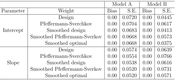
We consider two parameters: β0 and β1. Table 1 presents the Monte

Carlo biases and standard errors of the five point estimators considered. All the point estimators considered are found to be nearly unbiased. In term of efficiency, the estimators using smoothed weights are generally more efficient than the estimators using the original weights. The smoothed Pfeffermann-Sverkov estimator and smoothed optimal estimator perform similarly under Model A, since the homoscedasticity in the error variance makes the former estimator nearly optimal. On the other hand, under model B, the smoothed Pfeffermann-Sverchkov estimator is markedly inferior because it does not take into account unequal variances. In addition to point estimation, we have also computed variance estimators using the linearization method discussed in Section 5. All the variance estimators show negligible relative biases, less than 5% of the absolute values.

(25)

Table 1. Properties of alternative weighted point estimators in Simulation 1, based on 2,000 Monte Carlo samples

Model A Model B Parameter Weight Bias S.E. Bias S.E.

Design 0.00 0.0720 0.00 0.0445 Pfeffermann-Sverchkov 0.00 0.0704 0.00 0.0617 Intercept Smoothed design 0.00 0.0683 0.00 0.0413 Smoothed Pfeffermann-Sverkov 0.00 0.0668 0.00 0.0573 Smoothed optimal 0.00 0.0668 0.00 0.0375 Design 0.00 0.0574 0.00 0.0639 Pfeffermann-Sverchkov 0.00 0.0554 0.00 0.0766 Slope Smoothed design 0.00 0.0538 0.00 0.0616 Smoothed Pfeffermann-Sverkov 0.00 0.0520 0.00 0.0731 Smoothed optimal 0.00 0.0520 0.00 0.0571

7.2 Simulation 2

In the second simulation study a finite population of size N = 10,000 was generated with values (xi, yi, πi), where xi ∼ N(4,1), yi ∼ Bernoulli(pi),

logit(pi) = β0 +β1xi, (β0, β1) = (−2,1) and

πi =

exp (−4 + 0.3xi+ 0.3yi+ 0.3ui)

1 + exp (−4 + 0.3xi+ 0.3yi+ 0.3ui),

where ui ∼ N(0,1). From the finite population, we repeatedly generated

B = 2,000 samples by Poisson sampling where the sample indicatorIifollows

a Bernoulli(πi) distribution. The average sample size in this study is about

787.

For each sample, we computed five estimators of (β0, β1) by solving

N

X

i=1

(26)

where logitp(xi;β) =β0+β1xi and the alternative choices of weights wi are

as follows:

1. design weightsdi;

2. Pfeffermann-Sverchkov semiparametric weights diqi, where qi =

1/E(di |xi, Ii = 1) was obtained using (20);

3. smoothed design weights ˜di computed using (18);

4. smoothed Pfeffermann-Sverkov weights ˜diqi, where qi = 1/E(di |

xi, Ii = 1) was obtained using (20), as in Simulation 1;

5. smoothed optimal weights using the EM-type algorithm (32), as dis-cussed in Example 6.1.

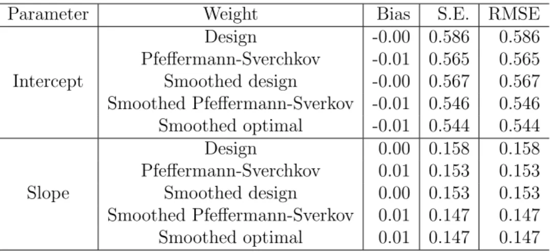
Table 2 presents the Monte Carlo biases, standard errors, and root mean squared errors of the five weighted estimators of β0 and β1 considered. As

expected, the smoothed optimal estimator shows the smallest standard er-ror. Variance estimators computed from (33) were all nearly unbiased in the simulation.

8 Concluding Remarks on Robustness

We have shown how the efficiency of weighted estimation of regression coef-ficients under informative sampling may be improved by two approaches to modifying the survey weights: smoothing and multiplication by a function of the covariate values. Both approaches, in their optimal forms, depend on fitting an auxiliary regression model to the weights. An important difference

(27)

Table 2. Properties of alternative weighted estimators in Simulation 2, based on 2,000 Monte Carlo samples

Parameter Weight Bias S.E. RMSE Design -0.00 0.586 0.586 Pfeffermann-Sverchkov -0.01 0.565 0.565 Intercept Smoothed design -0.00 0.567 0.567 Smoothed Pfeffermann-Sverkov -0.01 0.546 0.546 Smoothed optimal -0.01 0.544 0.544 Design 0.00 0.158 0.158 Pfeffermann-Sverchkov 0.01 0.153 0.153 Slope Smoothed design 0.00 0.153 0.153 Smoothed Pfeffermann-Sverkov 0.01 0.147 0.147 Smoothed optimal 0.01 0.147 0.147

between the approaches is that the consistency of estimation of the regression coefficients of interest depends on specifying the weight model correctly for the smoothing approach, but holds under arbitrary misspecification of the weight model for the second approach.

We conclude that weight smoothing is only likely to be appealing in prac-tice if the gain in efficiency it offers is appreciably superior to that offered by the second approach alone. The simulation studies illustrate how this may be the case. An illustration of how this may not be the case is provided by a common kind of survey of businesses or organizations where the principal source of variation in inclusion probabilities is the size of the organization. If this size variation is captured well by the x vector then smoothing is un-likely to offer much additional gain. For example, Fuller (2009, Example 6.3.3) analyses data from the Canadian Workplace and Employee Survey where disproportionate stratification is applied according to a measure of

(28)

size based on 1998 tax records. A single x variable is based on the total employment at the workplace in 1999, which captures a major source of vari-ation in the weights. Fuller (2009) finds that the second approach to weight modification does provide appreciable gains compared to a design-weighted approach. We find, when analysing these data, that there is little to be gained further by weight smoothing. Indeed, Fuller (2009) shows that the standard errors achieved by the second approach are close to those for un-weighted least squares and, since this effectively represents a lower bound, smoothing will be unable to do any better.

A further consideration is the question of robustness of these approaches under misspecification of the underlying regression model of interest. Under such misspecification, the alternative weighting methods will no longer pro-vide consistent estimation of a common parameter. The different weighted estimators will, in general, converge to different limits. Comparison of the different weighting approaches will therefore need to take account of both the appropriateness of these different limits as well as efficiency. We suggest that the appropriateness of limits will depend on the nature of the scientific application and that none of these approaches will always be superior in this respect, in line with the conclusion drawn by Scott and Wilde (2002) in the case of logistic regression modelling of case-control data.