Graduate Theses, Dissertations, and Problem Reports
2011
Development of an Artificial Neural Network to Predict In-Use
Development of an Artificial Neural Network to Predict In-Use
Engine Emissions
Engine Emissions
Melissa L. MorrisWest Virginia University
Follow this and additional works at: https://researchrepository.wvu.edu/etd Recommended Citation
Recommended Citation
Morris, Melissa L., "Development of an Artificial Neural Network to Predict In-Use Engine Emissions" (2011). Graduate Theses, Dissertations, and Problem Reports. 3086.
https://researchrepository.wvu.edu/etd/3086
This Dissertation is protected by copyright and/or related rights. It has been brought to you by the The Research Repository @ WVU with permission from the rights-holder(s). You are free to use this Dissertation in any way that is permitted by the copyright and related rights legislation that applies to your use. For other uses you must obtain permission from the rights-holder(s) directly, unless additional rights are indicated by a Creative Commons license in the record and/ or on the work itself. This Dissertation has been accepted for inclusion in WVU Graduate Theses, Dissertations, and Problem Reports collection by an authorized administrator of The Research Repository @ WVU. For more information, please contact [email protected].
Development of an Artificial Neural Network to Predict In-Use Engine Emissions
Submitted by: Melissa L. Morris
Dissertation submitted to the College of Engineering and Mineral Resources Doctor of Philosophy in Mechanical Engineering
at West Virginia University
Mechanical and Aerospace Engineering Department Morgantown, WV 26505-6106
Committee Members:
Dr. John Nuszkowski, Committee Chairperson Dr. Kenneth Means
Dr. W. Scott Wayne Dr. Gregory Thompson
Mr. Samuel Ameri
Keywords: Artificial Neural Network, Emissions Prediction, Road Grade
Copyright 2011
Abstract
A method to predict in-use diesel engine emissions is developed based on engine dynamometer and in-use data acquired at the West Virginia University Center for Alternative Fuels, Engines, and Emissions. (WVU CAFEE). The model accounts for the effects of road grade on generated emissions; a need for this model is evident in literature. Current modeling methods do not account for the effects of road grade, and have been shown to under-predict NOx by as much as 57%. It is determined through present research and a review of relevant literature that an artificial neural network (ANN) was the most applicable modeling method.
A modular ANN was developed to predict the heavy duty diesel engine emissions. The two modules were trained independently, the first module was trained with data acquired through in-use testing, and the second module was trained with data acquired via engine dynamometer testing. The first module predicted the engine speed and torque associated with the inputs of road grade and vehicle speed, while the second ANN employed the first ANN's outputs, and predicts the emitted quantities of NOx, CO2, HC, and CO. A series of training and verification
runs are conducted in order to determine the optimum ANN characteristics. Once the ANN was finalized, it was trained with and employed to predict the emissions associated with a variety of routes.
When the ANN was trained with a combination of in-use and engine dynamometer data, the ANN is able to predict NOx emissions associated with that same route within 6% of the measured values. The average difference between the measured and predicted CO2 values for
the same training and verification scenario mentioned above was less than 15%. It was also demonstrated that the ANN was able to predict emissions that are associated with routes that differ from those by which it is trained. When the ANN was trained with in-use data from a specific route, it was able to predict the NOx and CO2 emissions associated with a different route
with percent differences from the measured values of 20% or less.
Development of an Artificial Neural Network to Predict In-Use Engine Emissions
iii
Dedication
This dissertation is dedicated to my father; he inspired me to be where I am today. I hope one day to be as well respected and successful as he is as a faculty member, a parent, and a person in general.
iv
Acknowledgements
I would like to thank my advisor, Dr. John Nuszkowski, for being the best advisor ever! I am also grateful to my committee members, Dr. Gregory Thompson, Dr. Kenneth Means, Dr. W. Scott Wayne, and Mr. Samuel Ameri for their time and input. I would like to express a special thanks to Dr. Thompson for always being there to listen to my rants and rambles and encouraging me along the way. Dr. Means also deserves special recognition for supporting me through the duration of my graduate school experience and providing me with opportunities to work with students through his senior design courses.
I also would like to thank my parents, Gary and Lynn Morris, for being supportive and encouraging throughout my education. I especially thank them for instilling their values in me, and molding me into the person I am today.
My former students also deserve recognition; they are the main source of motivation for my pursuit of a doctorate degree. One student in particular, Justin Heydon, served as an inspiration and has provided me with constant encouragement and friendship over the past year.
I also would like to thank Jackson Wolfe, I am grateful to Jackson for always making me smile, for all of the great times we have had, and for those yet to come.
v
Table of Contents
List of Figures ... viii
List of Tables ... xiv
Nomenclature ...xvii
1. Introduction, Objectives, and Contributions ...1
1.1 Introduction ...1 1.2 Objectives ...5 1.3 Technical Approach ...5 2. Literature Review...7 2.1 Current Models ...7 2.1.1 MOBILE ...7 2.1.2 PSAT ...8 2.1.3 MOVES...8 2.1.4 IBIS ...9
2.1.5 Accuracy of MOBILE Model ...9
2.1.6 Accuracy of EMFAC Model ...11
2.1.7 Accuracy of Emissions Factor Models ...11
2.1.8 Emissions Inventory Estimation ...14
2.1.9 Modal Modeling Methods...14
2.2 Influencing Factors ...16
2.2.1 Deterioration Factor ...16
2.2.2 Road Grade ...17
2.3 Defeat Devices and Consent Decrees ...18
2.4 Artificial Intelligence Modeling Techniques ...18
2.4.1 Expert Systems...18
2.4.2 Bayesian Networks ...19
2.4.3 Genetic Algorithms ...19
2.4.4 Artificial Neural Networks ...20
vi
2.4.6 ANN Applied to Engine Optimization and Modeling ...29
3. Vehicle Testing and Data Collection ...33
3.1 In-Use Data Acquisition ...33
3.2 Test Engines ...34
3.3 Vehicle Routes ...35
3.3.1 Bruceton Mills, WV Route ...35
3.3.2 Washington, PA Route...40
3.3.3 In-Use Data Set Designations ...49
3.4 Engine Dynamometer Data Acquisition ...50
3.4.1 FTP Data ...51
3.4.2 Bruceton Mills, WV Cycle ...55
3.4.3 Washington, PA Cycle ...57
4. Repeatability of Measured Emissions Data ...60
4.1 Introduction ...60 4.2 Repeatability of an Engine ...60 4.3 Repeatability of a Vehicle ...63 4.4 Summary of Repeatability ...63 5. Model Development...64 5.1 Overview ...64 5.2 Model Architecture ...65 5.3 Road Grade ...65 5.4 Dispersion ...68 5.5 Vehicle Weight ...71 5.6 Deterioration ...76
5.7 Ambient Condition Effects ...79
5.8 Optimization ...81
5.8.1 ANN1 ...81
5.8.2 ANN2 ...85
5.8.3 Optimal Network ...86
6. Model Verification ...91
vii
6.2 Repeated Washington, PA Routes ...98
6.3 Same Engine, Different Routes...102
6.4 Same Route, Different Cycles...111
6.5 Comparison of Measured and Predicted Emissions to EPA Regulations ...119
6.6 HC and CO Predicted Values ...122
6.7 2002 Engine Emissions Predictions ...125
6.8 Same Route, Different Engines...136
6.9 Summary of Model Verification ...142
7. Significance...138
7.1 Impact of Road Grade ...145
8. Conclusions and Recommendations ...148
8.1 Conclusions ...148
8.2 Recommendations for Future Work...150
9. References ...151 Appendix ... A-1
viii
List of Figures
Figure 2.4.4.1: Schematic of Human Neuron ...21
Figure 2.4.4.2: Schematic of Artificial Neuron ...21
Figure 3.1.1: Schematic of MEMS ...34
Figure 3.3.1.1: Map of Bruceton Mills, WV Route ...36
Figure 3.3.1.2: Engine Speed for the Sabraton, WV to Bruceton Mills, WV Route with Manufacturer A Engine...37
Figure 3.3.1.3: Engine Torque for the Sabraton, WV to Bruceton Mills, WV Route with Manufacturer A Engine ...37
Figure 3.3.1.4: Road Grade from Sabraton, WV to Bruceton Mills, WV ...38
Figure 3.3.1.5: Engine Speed for Bruceton Mills, WV to Sabraton, WV Route with Manufacturer A Engine ...39
Figure 3.3.1.6: Engine Torque for the Sabraton, WV to Bruceton Mills, WV Route with Manufacturer A Engine ...39
Figure 3.3.1.7: Road Grade for Bruceton Mills, WV to Sabraton, WV ...40
Figure 3.3.2.1: Washington, PA 1 Route ...41
Figure 3.3.2.2: Engine Speed for Washington, PA 1 Route with Manufacturer A Engine ...42
Figure 3.3.2.3: Engine Torque for Washington, PA1 Route with Manufacturer A Engine ...42
Figure 3.3.2.4: Road Grade for the Washington, PA 1 Route ...43
Figure 3.3.2.5: Washington, PA 2 Route ...44
Figure 3.3.2.6: Engine Speed for Washington, PA 2 Route with Manufacturer A Engine ...44
Figure 3.3.2.7: Engine Torque for Washington, PA 2 Route with Manufacturer A Engine ...45
Figure 3.3.2.8: Road Grade for Washington PA 2 Route ...46
Figure 3.3.2.9: Washington, PA 3 Route ...47
ix
Figure 3.3.2.11: Engine Torque for Washington, PA 3 Route with Manufacturer B Engine ...48
Figure 3.3.2.12: Road Grade for Washington, PA 3 Route ...49
Figure 3.4.1: Schematic of Test Setup at EERC ...51
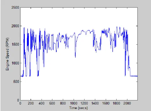
Figure 3.4.1.1: Manufacturer A Engine Speed During FTP Test ...52
Figure 3.4.1.2: Manufacturer A Engine Torque During FTP Test ...52
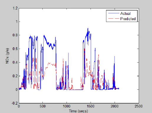
Figure 3.4.1.3: NOx Comparison When Emissions Module was Trained with FTP Data ...53
Figure 3.4.1.4: CO2 Comparison When Emissions Module was Trained with FTP Data ...54
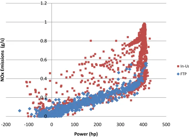
Figure 3.4.1.5 NOx Emissions versus Horsepower for Bruceton Mills, WV and FTP Engine Dynamometer Data ...55
Figure 3.4.2.1 Engine Speed for Sabraton, WV to Bruceton Mills, WV Engine Dynamometer Testing ...56
Figure 3.4.2.2: Engine Torque for Sabraton, WV to Bruceton Mills, WV Engine Dynamometer Testing...56
Figure 3.4.3.1: Engine Speed for Washington, PA Engine Dynamometer Testing ...57
Figure 3.4.3.2: Engine Torque for Washington, PA Engine Dynamometer Testing ...58
Figure 3.4.3.3: Engine Speed for Bruceton Mills, WV to Sabraton, WV Engine Dynamometer Testing ...59
Figure 3.4.3.4: Engine Torque for Bruceton Mills, WV to Sabraton, WV Engine Dynamometer Testing ...59
Figure 5.2.1: Basic Structure of Model ...65
Figure 5.3.1: Diagram of Relationship Between Distance Traveled and Altitude Change ...66
Figure 5.3.2: Height for Bruceton Mills, WV Route ...67
Figure 5.3.3: Road Grade for Bruceton Mills, WV Route ...67
Figure 5.5.1: Comparison of Predicted and Measured Engine Speed for Manufacturer B Engine ...74
Figure 5.5.2: Comparison of Predicted and Measured Engine Torque for Manufacturer B Engine without Correcting for Weight Difference Between Training and Verification Vehicles ...75
x Figure 5.5.3: Comparison of Scaled and Predicted Engine Torque for Manufacturer B Engine
when Correcting for Weight Difference Between Training and Verification Vehicles ...75
Figure 5.6.1: NOx Emissions versus Odometer Reading ...78
Figure 5.6.2: CO2 Emissions versus Odometer Reading ...79
Figure 5.7.1: NOx Emissions versus Temperature ...80
Figure 5.7.2: CO2 Emissions versus Temperature ...81
Figure 5.8.3.1: ANN1 Inputs and Outputs ...87
Figure 5.8.3.2: ANN2 Inputs and Outputs ...87
Figure 5.8.3.3: Tan-Sigmoid Transfer Function Plot ...88
Figure 5.8.3.3: Vehicle ANN, ANN1, Neuron Layer Structure ...89
Figure 5.8.3.4: Emissions ANN, ANN2, Neuron Layer Structure ...90
Figure 6.1.1: Vehicle ANN Predicted and Actual Engine Torque When Training with and Predicting Bruceton2Sab 2 Data Set ...94
Figure 6.1.2: Vehicle ANN Predicted and Actual Engine Speed When Training with and Predicting Bruceton2Sab 2 Data Set ...94
Figure 6.1.3: Difference Between Predicted and Measured Engine Speed for Run Sab2Bruceton 2 Verification Data ...95
Figure 6.1.4: Difference Between Predicted and Measured Engine Torque for Run 1 Sab2Bruceton 2 Verification Data ...96
Figure 6.1.5: Difference Between Predicted and Measured NOx Emissions for Run 1 Sab2Bruceton 2 Verification Data ...97
Figure 6.1.6: Difference Between Predicted and Measured CO2 Emissions for Run 1 Sab2Bruceton 2 Verification Data ...93
Figure 6.2.1: Difference Between Predicted and Measured Engine Speed for the Washington, PA Route When Trained with Washington, PA2 1 ...100
Figure 6.2.2: Difference Between Predicted and Measured Torque for the Washington, PA Route When Trained With Washington, PA2 1 ...100
xi Figure 6.2.3: Difference Between Predicted and Measured NOx for the Washington, PA Route When Trained with Washington, PA2 1 and ...101 Figure 6.2.4: Difference Between Predicted and Measured CO2 for the Washington, PA Route
When Trained with Washington, PA2 1 ...102 Figure 6.3.1: Difference Between Predicted and Measured Engine Speed for the Sabraton, WV to Bruceton Mills, WV Route When ANN was Trained with Washington, PA2 1 ...104 Figure 6.3.2: Difference Between Predicted and Measured Engine Torque for the Sabraton, WV to Bruceton Mills, WV Route When ANN was Trained with Washington, PA2 1 ...105 Figure 6.3.3: Difference Between Predicted and Measured NOx for the Sabraton, WV to Bruceton Mills, WV Route When ANN was Trained with Washington, PA2 1 ...105 Figure 6.3.4: Difference Between Predicted and Measured CO2 for the Sabraton, WV to
Bruceton Mills, WV Route When ANN was Trained with Washington, PA2 1 ...106 Figure 6.3.5: Difference Between Predicted and Measured Engine Speed for the Bruceton2Sab 1 Route ...107 Figure 6.3.6: Difference Between Predicted and Measured Engine Torque for the Bruceton2Sab 1 Route ...109 Figure 6.3.7: Difference Between Predicted and Measured NOx for the Bruceton2Sab 1 Route ...110 Figure 6.3.8: Difference Between Predicted and Measured CO2 for the Bruceton2Sab 1 Route
...110 Figure 6.4.1: Difference Between Predicted and Measured Engine Speed for the Sab2Bruceton 1 Data Set ...112 Figure 6.4.2: Difference Between Predicted and Measured Engine Torque for the Sab2Bruceton 1 Data Set ...113 Figure 6.4.3: Difference Between Predicted and Measured NOx for the Sab2Bruceton 1 Data Set ...114 Figure 6.4.4: Difference Between Predicted and Measured CO2 for the Sab2Bruceton 1 Data Set
...114 Figure 6.4.5: Difference Between Predicted and Measured Engine Speed for the Washington PA1 When ANN Was Trained With Washington PA2 1 Route ...116
xii Figure 6.4.6: Difference Between Predicted and Measured Engine Torque for the Washington PA1 When ANN was Trained With Washington PA2 1 Route...117 Figure 6.4.7: Difference Between Predicted and Measured CO2 Emissions for the Washington
PA1 When ANN was Trained With Washington PA2 1 Route...118 Figure 6.4.8: Difference Between Predicted and Measured NOx Emissions for the Washington PA1 When ANN was Trained With Washington PA2 1 Route...118 Figure 6.7.1: : Predicted and Measured Engine Speed for Washington PA1 When the ANN was Trained with Data from Washington PA2 Route ...127 Figure 6.7.2: Predicted and Measured Torque for Washington PA1 When the ANN was Trained with Data from Washington PA2 Route ...128 Figure 6.7.3: Predicted and Measured NOx Emissions for Washington PA1 When the ANN was Trained with Data from Washington PA2 Route ...129 Figure 6.7.4: Predicted and Measured CO2 Emissions for Washington PA1 When the ANN was Trained with Data from Washington PA2 Route ...129 Figure 6.7.5: Predicted and Measured Engine Speed for Sabraton, WV to Washington, PA When the ANN was Trained with Data from Washington, PA3 to Sabraton, WV Route ...130 Figure 6.7.6: Predicted and Measured Torque for Sabraton, WV to Washington, PA When the ANN was Trained with Data from Washington, PA3 to Sabraton, WV Route ...131 Figure 6.7.7: Predicted and Measured NOx Emissions for Sabraton, WV to Washington, PA When the ANN was Trained with Data from Washington, PA3 to Sabraton, WV Route ...132 Figure 6.7.8: Predicted and Measured CO2 Emissions for Sabraton, WV to Washington, PA
When the ANN was Trained with Data from Washington, PA3 to Sabraton, WV Route ...132 Figure 6.7.9: Predicted and Measured NOx Emissions for Sabraton, WV to Washington, PA When the ANN was Trained with Data from Washington, PA3 to Sabraton, WV Route ...134 Figure 6.7.10: Predicted and Measured CO2 Emissions for Sabraton, WV to Washington, PA
When the ANN was Trained with Data from Washington, PA3 to Sabraton,WV Route ...134 Figure 6.7.11: Predicted and Measured NOx Emissions for Sabraton, WV to Washington, PA When the ANN was Trained with Data from PA3 to Sabraton, WV Route ...135 Figure 6.7.12: Predicted and Measured CO2 Emissions for Washington, PA to Sabraton, WV
xiii Figure 6.8.1: Predicted and Measured NOx Emissions for Washington, PA to Sabraton, WV When the ANN was Trained with Data from Sabraton, WV to Washington, PA Route ...138 Figure 6.8.2: Predicted and Measured CO2 Emissions for Bruceton Mills, WV route When the
ANN was Trained with Data from Washingtonington, PA 2 Route ...139 Figure 6.8.3: Predicted and Measured NOx Emissions for Bruceton Mills, WV route When the ANN was Trained with Data from Washington, PA 2 Route ...141 Figure 6.8.4: Predicted and Measured CO2 Emissions for Washington, PA route When the ANN
xiv
List of Tables
Table 1.1.1: Emissions Regulations ...3
Table 2.4.3.1: Genetic Algorithm Approach ...20
Table 2.4.4.1: Commonly Used Transfer Functions in ANN ...24
Table 2.4.6.1: Engine Operating Parameters Used As Inputs to Genetic Algorithm ...30
Table 3.2.1: Manufacturer A Engine Specifications ...35
Table 3.2.2: Manufacturer B Engine Specifications ...35
Table 3.2.3: Manufacturer C Engine Specifications ...35
Table 3.3.3.1: Data Set Designations ...50
Table 4.2.1: Statistical Analysis of MEMS Data Summary for Manufacturer A Engine ...61
Table 4.2.2: Statistical Analysis of MEMS Data Summary for Manufacturer D Engine ...62
Table 4.2.3: Statistical Analysis of MEMS Data for All Engines ...62
Table 4.3.1: Comparison of Different Engines of the Same Engine Model on the Same Route ..63
Table 5.5.1: Comparison of Measured and Predicted Emissions Values for Lighter Weight when Weight Difference is Considered and Not Considered ...76
Table 5.8.1.1: Optimization of the ANN1 ...83
Table 5.8.1.2: Optimization of the ANN2 ...84
Table 6.1.1: Verification of ANN for Training with, and Predicting Bruceton Mills, WV Routes ...93
Table 6.2.1: Verification of ANN for Training with, and Predicting Washington, PA Routes ....99
Table 6.3.1: Verification of ANN for Trained with Washington, PA and Used for Prediction of Bruceton Mills, WV Routes ...103
Table 6.3.2: Verification of ANN Trained with Washington, PA Data and Used for Prediction of Bruceton Mills, WV Routes ...108
Table 6.4.1: Verification of ANN Trained with Bruceton Mills, WV Data and Used for Prediction of Bruceton Mills, WV Routes ...111
xiv Table 6.4.2: Verification of ANN Trained With Washington, PA Data and Used for Prediction of Washington, PA Routes ...115 Table 6.5.1: Predicted Values, Measured Values, and EPA Regulations for ANN Trained with Bruceton2Sab 1 and Washington, PA1 Engine Dynamometer Data ...120 Table 6.5.2: Comparison of Predicted Values and Measured Values to EPA Regulations for ANN Trained with Bruceton2Sab 1 and Washington, PA1 Engine Dynamometer Data ...120 Table 6.5.3: Predicted Values, Measured Values, and EPA Regulations for ANN Trained with Washington, PA2 1 and Bruceton Mills, WV Engine Dynamometer Data ...121 Table 6.5.4: Comparison of Predicted Values and Measured Values to EPA Regulations for ANN Trained with Washington, PA2 1 and Bruceton Engine Dynamometer Data ...122 Table 6.6.1: Predicted and Measured Values for HC and CO for ANN Trained with Washington, PA2 1 and Sabraton, WV to Bruceton Mills, WV Engine Dynamometer Data ...123 Table 6.6.2: Comparison of Predicted Values of CO and HC to Measured Values from Engine Dynamometer Data for ANN Trained with Washington, PA2 1 and Bruceton Engine Dynamometer Data ...124 Table 6.6.3: Predicted and Measured Values for HC and CO for ANN Trained with Bruceton2Sab 1 and Washington, PA1 Engine Dynamometer Data ...124 Table 6.6.4: Comparison of Predicted Values of CO and HC to Measured Values from Engine Dynamometer Data for ANN Trained with Bruceton2Sab 1 and Washington, PA1 Engine Dynamometer Data ...125 Table 6.7.1: Comparison of Predicted and Measured Values of NOx and CO2 for the ANN
Trained with In-Use Data ...126 Table 6.7.2: Comparison of Predicted and Measured Values of NOx and CO2 for the ANN
Trained with In-Use Data ...133 Table 6.8.1: Comparison of Measured and Predicted Emissions when the ANN was Trained with a 400 hp Engine and Used to Predict a 350 hp Engine ...138 Table 6.8.2: Comparison of Measured and Predicted Emissions when the ANN was Trained with a 400 hp Engine and Used to Predict a 350 hp Engine ...140 Table 6.9.1: Confidence Interval Summary for Manufacturer A 400 hp Engine ...143 Table 6.9.2: Confidence Interval Summary for Manufacturer A 350 hp Engine, Manufacturer B Engine, and Manufacturer C Engine ...143
xvi Table 7.1.1: Emissions Predicted without Road Grade as an Input ...147
xvii
Nomenclature
ANN Artificial Neural Networks
bhp Brake Horsepower
CAA Clean Air Act
CARB California Air Resource Board
CBD Central Business District
CO Carbon Monoxide
CO2 Carbon Dioxide
COV Coefficient of Variance
EGR Exhaust Gas Recirculation
EPA Environmental Protection Agency
FOREMORE Forecast of Emissions from Motor Vehicles
FTP Federal Test Procedure
g Grams
GA Genetic Algorithm
HC Hydrocarbons
hp Horsepower
IBIS Integrated Bus Information System MEMS Mobile Emissions Measurement System MOVES Motor Vehicle Emissions Simulator
NOx Oxides of Nitrogen
ODEE On-Road Diesel Emissions Characterization
PM Particulate Matter
ppm Parts per Million
PSAT Powertrain System Analysis Toolkit
SCF Speed Correction Factor
1
1. Introduction, Objectives, and Contributions
1.1 Introduction
Since the early 1960's regulations have been implemented concerning exhaust emissions from heavy duty trucks and buses, specifically with diesel engines. The regulations are concerned with limiting the quantities of gaseous and particulate emissions from heavy duty diesel vehicles. In 1973, the first regulations were implemented to limit the quantity of oxides of nitrogen (NOx), carbon monoxide (CO), and hydrocarbons (HC), it was not until 1988 that a regulation included limits on the amount of particulate matter (PM) emitted [1]. As researchers became more aware of the health and environmental effects of diesel engine emissions, more strict emission regulations have been implemented.
Carbon monoxide is an odorless, invisible gas that is a result of incomplete combustion. Carbon monoxide can cause nausea, headache, and in high enough doses, death. Hydrocarbons are the result of unburned or partially burned fuel. Since diesel fuel is a compound consisting mainly of hydrogen and carbon, the unburned carbon and hydrogen atoms are free to form hydrocarbons [2]. PM is often visible to the human eye as smoke; however it is more frequently present as fine particles which are not visible. It is the small particles that have the greatest negative impact on individuals who are exposed to diesel engine exhaust. Particulate matter is not only an esthetic nuisance, it is also responsible for health issues. The American Lung Association and California Air Resource Board (CARB) have stated that 15,000 premature deaths annually can be attributed to particulate matter produced from diesel engines [3]. Also it has been shown that children who are exposed to PM have reduced lung function and a higher occurrence of asthma related issues. The fine particles pass through the membranes of human lungs, resulting in them becoming imbedded in deep pockets of the lungs, which can hinder biological processes [3]. Other health issues that have been attributed to PM exposure include coughing, decreased lung function, weakening of the heart, breathing difficulty, and aggravated pre-existing conditions. Individuals who already suffer from asthma, bronchitis, and emphysema are more susceptible to experience the effects of PM [2]. NOx is the term given to combinations of oxygen and nitrogen atoms, and is of concern to the environment due to its contribution to ground-level ozone when it reacts with hydrocarbons and sunlight. Ozone is the main constituent in smog, which results in limited visibility and negative health effects. Increased permeability of lung tissue is one of the known
2 effects of ozone exposure. When lung tissue is more permeable, toxins and bacteria are more likely to enter and remain in the lungs [4]. Individuals who are already plagued by allergies become more susceptible to allergens due to this increased permeability [5]. Aside from the above mentioned health effects, diesel engine emissions also contribute to the occurrence of acid rain and the greenhouse gas inventory. In order to understand the breadth of the negative impacts of diesel engine emissions, the quantity of these particular constituents attributed to diesel engine emissions must be determined.
The EPA has estimated that heavy-duty diesel vehicles contribute sixty percent of the on-road particulate matter emissions and twenty-seven percent of the on-road NOx emissions [6]. Other sources have estimated that heavy duty diesel engines are responsible for between thirty and sixty percent of on-road NOx emissions [7]. These high percentages are particularly important because heavy-duty diesel vehicles only make up two percent of the on-road traffic [6]. The uncertainty in the quantity of emissions contributed by heavy duty diesel engines is due to a limited understanding of the effects of test cycle, deterioration, and engine programming on in-use emission rates [9]. In order to reduce the health and environmental impact of diesel engine emissions, the allowable levels of emission constituents have been reduced.
The current, more stringent emission regulations only apply to newly manufactured engines. Engines that are already in service are not required to conform to new emission standards. Since older engines are still in use, it is necessary to have a means by which to predict their emissions in order to accurately arrive at an emission inventory value. According to the EPA, engines currently in operation, which are not required to meet new standards, may still be in operation for the next 25 to 30 years [4]. Table 1 displays the emission regulations from 1988 to the present. Between 1988 and 1998 the allowable emission values were regulated differently for trucks and buses, since 2002 both trucks and buses must meet the same standards. It is shown that over the years acceptable emissions levels have decreased, by one to two orders of magnitude.
3 Table 1.1.1: Emissions Regulations [10]
Trucks Emission Constituent (g/bhp-hr) Year HC CO NOx PM 1988 1.3 15.5 10.7 0.6 1990 1.3 15.5 6 0.6 1991 1.3 15.5 5 0.25 1994 1.3 15.5 5 0.1 1998 1.3 15.5 4 0.1 Urban Buses Emission Constituent (g/bhp-hr) Year HC CO NOx PM 1991 1.3 15.5 5 0.25 1993 1.3 15.5 5 0.1 1994 1.3 15.5 5 0.07 1996 1.3 15.5 5 0.05 1998 1.3 15.5 4 0.05
Both Trucks and Buses
Emission Constituent (g/bhp-hr) Year NMHC CO NMHC+NOx PM 2002 Option 1 NA 15.5 2.4 0.1 2002 Option 2 0.5 15.5 2.5 0.1 Emission Constituent (g/bhp-hr) Year NMHC CO NOx PM 2007/2010 0.14 15.5 0.2 0.01
Currently, multiple methods exist for modeling and predicting emissions data. The simplest emissions estimation method employs look-up tables of previously obtained emissions data. Two of the most commonly used methods rely on continuous axle power, speed and torque data. The method of using vehicle speed to predict exhaust emissions employs an average schedule speed and what are known as speed correction factors (SCFs). It is common practice for the value of the SCF to be one at the average schedule speed. The SCFs are determined by examining the relationship between speed and the emission constituent of concern. Once the correction factors are determined, emissions from a test schedule with a different average speed can be predicted based on the emissions from the modeled test schedule. It has been shown that this modeling method does not produce consistently accurate results. Error is introduced when
4 two test schedules have similar average speeds, but different variations in the speed levels during the schedule [11].
The method of using vehicle power to predict exhaust emissions requires continuous emissions data and axle power data. This method relies on a curve fit between the instantaneous emissions and power at the axle. The function associated with the curve fit is then used to predict emissions based on the axle power of other test schedules. Using axle power to predict NOx emissions does not provide accurate results, and should only be used in cases where rough estimates are sufficient [11]. Ramamurthy et al. also researched predicting diesel engine emissions by correlating axle power to emissions. CO, NOx, and CO2 were plotted as functions
of axle power, and curves were fitted to the data. Once correlations were formed, the functions were used to predict emissions data associated with various test cycles. It was determined by these researchers that axle power is a sufficient predictor of CO2 and NOx emissions; however,
the prediction of CO emissions based on axle power was inaccurate. Discrepancies between the predicted and experimentally obtained emission values can result if the cycle used to establish the correlation between the emission constituent and axle power does not span the full range of power for the specific vehicle being examined [12].
Joumard et al. addressed the possible errors and issues encountered when modeling in-use emissions. Many models rely on average speed to predict emissions over a driving cycle, however this can introduce error in predicted emissions because it has been shown that significant changes in speed can impact instantaneous emissions by two to three times. Errors are also incorporated into emissions modeling via measurement errors and modeling errors. When data is recorded, it is important to be sure measurement and recording instrumentation is functioning as expected. It is also important to document environmental conditions, due to their impact on emissions levels. Modeling errors may occur if inadequate parameters are employed by the model, resulting in the model not accurately predicting emissions from the applied database. The researchers recommend in order to accurately predict emissions, both instantaneous operating conditions and an operating condition history should be considered [13].
5 1.2 Objectives
The global objective of this dissertation work was to develop a model that can accurately predict in-use heavy duty diesel engine emissions by employing engine dynamometer data available through the previous work of the West Virginia University, CAFEE. The major objectives that led to the accomplishment of the global objective are listed below.
Identify most applicable and effective modeling method.
Develop an emissions model that can predict in-use emissions from engine dynamometer data.
Verify the model by comparing results with experimental data and EPA regulations. Present a final working model to accurately predict in-use emissions
1.3 Technical Approach
The work required to achieve the above mentioned objectives was divided into the tasks explained below.
A. Literature Review
Conducted a review of literature pertaining to heavy duty diesel engine emissions research, standards, modeling, and prediction methods.
B. Data Survey
Located and determined availability of engine dynamometer data for heavy duty diesel engines employed in trucks and buses. Determined the availability of in-use data for model verification.
C. Model Development
Determined the optimum modeling method and developed a model that accurately predicts in-use heavy duty diesel emissions from engine dynamometer data, taking into account grade effects.
Problem Definition and Formulation
o Defined desired output and determined required inputs System Design
o Determined structure for ANN
6 o Collected and pre-processed data
System Realization
o Trained ANN with specified data o Evaluated initial outputs and errors
D. Model Optimization
Varied model characteristics in order to reach the most accurate predictions of in-use emissions data.
E. Model Verification
Compared model output results to actual in-use data in order to determine the model’s accuracy.
7
2. Literature Review
2.1 Current Models
Currently, few widely used computer models exist for predicting emission inventories and in-use emissions from heavy duty diesel vehicles. The Environmental Protection Agency (EPA) and the California Air Resource Board (CARB) are the agencies most concerned with emissions modeling in the United States. The most commonly used models are EPA's MOBILE, CARB's EMFAC, and EPA's MOVES. The EPA also employs particulate matter estimation models known as PART5 and PART6. CARB’s prediction methods are based on engine certification data and a limited number of chassis dynamometer tests [14]. The EPA also developed the Mobile Emission Assessment System for Urban and Regional Evaluation, known as MEASURE. MEASURE was developed in the late 1990s, in order to predict the effect of suburban sprawl and commuting to metropolitan areas on emissions. The purpose of the program was to aid transportation designers in analyzing the impacts of actions such as signal timing and adding lanes [15]. The most recently released emission model developed by the EPA is MOVES2010, which replaced MOBILE6.2.
2.1.1 MOBILE
The EPA developed the first version of its MOBILE software in the 1970s, it was denoted as MOBILE1. Since its inception, the MOBILE model has been updated with releases MOBILE2, MOBILE3, MOBILE4, MOBILE 4.1, MOBILE5, MOBILE5a, MOBILE5b, MOBILE6 and MOBILE6.2. The Clean Air Act (CAA) requires the EPA to update the emissions estimation programs, and release currently applicable versions. With each release, the models have included more in-use data, have been updated to be compatible with new technologies, and have accounted for more factors when estimating engine emissions. MOBILE1 was released in 1978, and used age and mileage of vehicles in order to arrive at estimated emission values. MOBILE2 and MOBILE3, released in 1981 and 1984, respectively, took into account newer vehicle technologies including catalytic converters and the effect of tampering. New in-use data and more user control options were incorporated into MOBILE4, released in 1989. MOBILE4.1 was released in 1991 and incorporated the effects of operation and maintenance programs, as well as the impact of the newest emissions regulations. Due to state implemented test programs, a larger data set was available and new equations were derived to predict emissions for the 1993 release
8 of MOBILE5 and MOBILE5a. The impacts of oxygenated and reformulated fuels on emissions were also examined in the MOBILE5 series. In 1996 MOBILE5b was released which was updated to include the newest emission regulations, and the ability to estimate idle emission factors was included. The release of MOBILE6.0 occurred in 2002, and the new program was equipped with more in-use deterioration data, and updated for newer engine and fuel technologies. The ability to model air toxins such as benzene and formaldehyde and improved carbon monoxide prediction values were features of the MOBILE6.2 program, released in 2004 [16].
2.1.2 Powertrain System Analysis Toolkit
The United States Department of Energy has contributed to the development of modeling software based in MATLAB, which is called Powertrain System Analysis Toolkit (PSAT). PSAT is a vehicle simulation toolkit that estimates vehicle performance from a calculated component torque response to realistic commands. This software is widely used in the automotive industry for vehicle simulations and modeling. Inputs such as engine throttle, clutch displacement, and transmissions gear number are employed in the software. PSAT is capable of modeling a variety of vehicle technologies including conventional, electric, fuel cell, and hybrid. PSAT is capable of accurately predicting emissions for heavy duty diesel engines over various cycles, however it requires extensive input information, some of which may not be known for vehicles that need to be modeled. For example, a vehicle may be equipped with a specific engine, but information about the transmission could be unavailable [55].
2.1.3 MOVES
As mentioned above, the EPA plans to replace the MOBILE series of emission prediction programs with a newly developed program called Motor Vehicle Emissions Simulator, also known as MOVES. MOVES2010 includes more in-use data than the previous MOBILE series and is also able to predict the emission levels of more Volatile Organic Compounds (VOCs). Initial comparisons of MOVES2010 to MOBILE6.2 show that MOVES2010 predicts lower values for emitted VOCs in urban areas, higher values for NOx emitted, and higher quantities of particulate matter emitted [17]. These differences in the two models show that there is still room for improvement and uncertainty in the emissions predictions modeling realm.
9 2.1.4 IBIS
Wayne et al. have developed a modeling tool to predict the emissions associated with fleets of transit vehicles, this model titled, Integrated Bus Information System (IBIS), allows a user to determine the emissions associated with a particular fleet of vehicles. The use must enter information about the vehicles in the fleet being examined such as type of fuel, model year, curb weight, powertrain type, engine rated power, aftertreatment equipment, transmission type, heating and air-conditioning capacity, and displacement. For the route being examined, information such as the average speed, percentage idle, number of stops per mile, standard deviation of speed, and the kinetic intensity must be known. The model predicts the fuel economy, and emissions of NOx, CO2, CO, PM, and HC. The data employed to develop this
model was obtained from chassis dynamometer testing, and then polynomial fits and linear regressions were applied to the data. In cases where data were not available for a particular scenario, genetic algorithms were employed to predict the emissions for that situation. The purpose of this modeling tool is to allow fleet owners to compare and contrast the emissions associated with fleets of different characteristics, in order aid in planning and procurement decisions [66].
2.1.5 Accuracy of MOBILE Models
It has been determined through prior work that actual measured emissions data from heavy-duty diesel vehicles differ from the results that are predicted through the use of models such as MOBILE5 and PART5. The measured emissions values also differ from the data that has resulted from engine certification tests. One of the reasons it is important to accurately estimate the emissions from vehicles is to determine if the regulations that have been put into effect are making a difference. Also, in order to examine, monitor, and plan air quality, pollutant inventories are developed, which are based on the estimated emissions. In-use emissions are functions of driving cycle, inertial weight, and drive trains. Plots of NOx versus power were constructed and examined as part of the research of Yanowitz et al., and it was determined that it is possible to employ chassis testing and a transmission model to determined if in-use NOx emissions agree with the engine certification results. This work also concluded that emitted carbon monoxide (CO) values on a brake-specific mass basis agree between chassis and engine dynamometer tests. Particulate matter emissions were determined to be underestimated by
10 engine certification tests, when compared to chassis data on brake-specific mass basis [18]. Singh et al. also noted that current emissions prediction programs such as those discussed previously are only capable of predicting emission inventories at a county-size scale. It was the recommendation of the researchers that a program be developed that is able to predict PM emissions on a smaller scale, therefore the impact on humans and the environment at specific sites can be examined [19].
Studies have shown that PART5, the EPA's PM emission factor model, estimates PM production to be much less than what is actually emitted during in-use conditions. The PART5 program was revised to better estimate PM emissions, by examining the data produced by four test vehicles, two trucks and two buses. In order to make revisions to the PART5 model, the assumptions that the model employs were examined. It was shown that the PART5 model assumes that PM emissions from a vehicle will not ever exceed the level at which it was certified. This assumption introduces error by assuming that the technologies used to meet the new, more stringent emission standards will not deteriorate with time or fail. As the technologies get more complicated, resulting in a greater reduction of emissions, there is also the fact that if they fail to operate optimally, greater emissions than expected will result. A study by Whitney determined that the PART5 estimated PM emissions were three to 11 times lower than those actually emitted by light-duty vehicles, most specifically seen in vehicles with an excess of 100,000 miles [20]. It is suspected by researchers that the portion of NOx in emissions inventories attributed to heavy-duty diesel vehicles is under representing the actual contributions of these vehicles. The under-estimation is in part due to the fact that many emission inventories are estimated using data acquired during engine certification testing. One emission prediction model, MOBILE, employs engine certification data and has been shown to predict less NOx emissions than what tunnel and on-road testing have shown. One reason for this discrepancy is that engine producers were programming the engines to operate differently when they were noticeably running the FTP cycle for certification. When these engines were put into vehicles, they produced more emissions than they did during the certification testing. Since the MOBILE model and other emissions prediction models employ engine certification data, some of their predictions have been based on unrealistic data that was acquired during certification testing of these engines.
11 Engine manufacturers have since signed consent decrees, in which the manufacturers agreed to retrofit such engines during maintenance, pay fines, and comply to 2004 emissions standards earlier than was originally expected. As part of the consent decrees it was determined that a program would be developed to correlate in-use testing with engine certification data. A division of the EPA developed the On-Road Diesel Emissions Characterization (ODEC) facility, which has the goal of compiling in-use emissions data for a variety of road conditions and vehicles [22].
2.1.6 Accuracy of EMFAC Model
Shah et al. compared the measured NOx emissions associated with various driving schedules to those that are estimated by EMFAC. The emissions were measured for eleven vehicles employing engines ranging from 1996 to 2000. It was determined that the EMFAC predictions underestimated the quantity of NOx emitted by five to fifty-seven percent, based on the test cycle being examined [21].
2.1.7 Accuracy of Emission Factor Models
McCormick et al. researched comparing data obtained from an engine dynamometer to data obtained from a chassis dynamometer, and evaluated the correlation. For this research two buses and a truck were tested on a chassis dynamometer and then the engines were removed from the vehicles and tested on engine dynamometers. The two transit buses were equipped with 1993 DDC Series 50 engines, while a truck was powered by a Navistar DTA-466 engine. The chassis dynamometer tests employed the CBD and HDT cycles. When the emissions data from the two cycles were compared, it was determined that when compared on a fuel volume basis the HDT and the CBD agreed closely, but when compared on a distance basis a significant disagreement in data was seen. This can be explained due to the effect of inertial weight on all emissions constituents when compared on a distance basis, but when the emissions values are compared on a volume basis, only PM is effected by the inertial weight. Emissions prediction factors in work per distance were then estimated by using the data obtained from these tests. These factors were used to convert engine dynamometer data to distance specific values and then these values were used to estimate emissions inventories. The factors that were determined from this research were then compared to the factors that are currently employed by the EPA in inventory estimation
12 methods, and it was found that the factors were substantially different. Accurate estimations of pollution inventories are necessary for air quality planning and determining the effectiveness of regulations. The discrepancy between the EPA estimated emissions factors and the ones determined in this work could be due to the fact that the EPA based its emission factors on the data acquired from engine certification testing. During engine certification testing, new engines are tested on engine dynamometers. In order to estimate the emissions produced by the engine over its lifetime (435,000 miles) a deterioration factor is employed. Engines are still in service that have accrued more than 435,000 miles, therefore assuming that engines are no longer operating after their lifetime is an error inducing assumption. Also, it has not been proven that the EPA's deterioration factor contributes to accurately predicting in-use emissions for all types of engines over their lifetimes. The current EPA factors are based on a comparison of engine and chassis dynamometer testing for a transit bus and three trucks. The emission factor is a ratio of the chassis dynamometer results to the engine dynamometer results [8]. Using engine certification data may also skew data in cases where the engines being tested are equipped with defeat devices. It is unclear if the deterioration factor accounts for lack of maintenance of turbochargers and fuel injectors, which leads to increased PM, HC, and CO emissions. Also it should be noted that an increase in NOx emissions can be attributed to improperly timed fuel injection or poor air cooler performance [23]. The above mentioned deterioration and maintenance issues are not measured during engine certification data and may not be properly accounted for in the deterioration factors used by the EPA, therefore further examination is needed.
Research has resulted in the development of a table of emissions factors that aid in the prediction of in-use emissions. The emission factors are based on instantaneous engine power. The model predicts emissions by employing a series of matrices for the exhaust constituents including NOx, CO, CO2, and HC, using the inputs of speed and acceleration. The PM emissions were estimated
by using a ratio of the known PM emission values over a speed and acceleration range, based on CO emissions. Data acquired via testing by the WVU Mobile laboratory were used to compile the matrices employed by the model. Multiple methods exist to estimate emission inventories, some include using engine certification data, data acquired by chassis dynamometer testing, and ratios of NOx and CO2. MOBILE5 and MOBILE6, the EPA's emission prediction models, and
13 EMFAC, CARB's model, are based on data used for engine certification. The FTP cycle does not adequately represent present day driving conditions such as stop-and-go city and freeway conditions, and therefore fails to accurately model the emissions of current vehicles. Using the engine certification data to model engine emissions also does not account for the deterioration, maintenance, and any alterations experienced by the engines. When chassis dynamometer data is used to predict emissions, inaccuracies result from that fact that specific cycles are used to analyze the emissions, and none of the cycles have the ability to model the multitude of driving conditions that a given vehicles will experience. Emission factors based on power allow the emissions to be predicted for a cycle other than the cycle which was used to acquire the data. Issues arise when using this method, because for it to be accurate, time alignment must occur that relates the instantaneous rear-axle power and the emissions. It is possible to measure the instantaneous power easily; however there is a delay between when the power event occurs and when the exhaust gas reaches the measuring instruments. For NOx and CO2 this prediction
method has been shown to be successful, however results have not been as promising for the prediction of CO and HC. Another downfall of predicting emissions based on rear-axle power is that the effect of "off-cycle" injection timing cannot be incorporated. In some cases speed and acceleration are used to predict emissions rather than instantaneous power. The speed is employed to determine losses due to road-load, and the acceleration coupled with the speed can predict the instantaneous inertial power demand. When a vehicle experiences a change in road grade, the effect on emissions is not well documented due to the lack of grade simulation in chassis dynamometer testing. The uncertainty in emissions associated with road-grade changes induces problems into the method of predicting emissions based on speed and acceleration data. When climbing an incline acceleration is low, however significant rear-axle power is required and when travelling in a descending direction acceleration can be high, while limited power is required. This results in the model over estimating emissions for descending terrains, and under estimating emissions when vehicles ascend hills. Along with speed and acceleration, weight also plays a key role in emissions prediction. It is important to account for the weight of a vehicle because the higher the load, generally the higher the emissions for a given speed and acceleration. When examining buses in particular this is a concern since the load of the bus can change with each stop, in the case of tractor-trailers, the load is typically constant over the length of a trip [24].
14 2.1.8 Emissions Inventory Estimation
It has been shown that emissions inventory estimation techniques do not account for every factor that impacts emission, and as shown in the reviewed literature, are not as accurate predictors of diesel engine emissions as they could be. Research has shown that emissions inventory estimations are based on data obtained from FTP tests, when engines are new and undergoing certification. In order to test older engines on engine dynamometers the engines must be removed from the vehicle, which requires the vehicle to be out of service during testing, and then time and money must be expended to reinstall the engine into the vehicle. The time involved and financial expense of dynamometer testing is the main reason that data for the emission inventory is limited. Concerns have also been raised, stating that the FTP is over 25 years old, and has not been updated to accurately assess the engines that are equipped with newer technologies. It is thought that data acquired by chassis dynamometer testing would better represent in-use emissions, when compared to the FTP data [25].
Data were obtained by the WVU Mobile Laboratories for emissions from buses and heavy duty trucks. Data for buses were determined by employing the Central Business District (CBD) cycle, while heavy duty trucks were examined with the truck CBD and the WVU 5-peak test cycle. Throughout the duration of the chassis dynamometer tests, the drag on the vehicle and rolling friction of tires were incorporated by taking into account the air density, the frontal area of the vehicle, the drag coefficient, and the friction coefficient. It was determined that the NOx measurements from the chassis tests were within the range of certification provided by FTP data, however the ratio of NOx to CO2 was found to be widely variable, which supports the opinion
that the FTP cycle is not always accurate in estimating in-use emissions [25]. 2.1.9 Modal Modeling Methods
Barth et al. believe that modeling emissions using a modal method will prove to be more accurate than the current methods used by the programs available through the EPA and CARB. Currently the modeling methods assume that it is accurate to use emissions measured from a specific driving cycle in cooperation with a speed correction factor to predict in use vehicle emissions. The authors of this work have shown the need for a model that considers events such as acceleration/deceleration, idle, and steady-state cruise. Currently emissions modeling
15 techniques do not account for realistic driving conditions; most models rely on data derived from the FTP cycle. The FTP cycle mimics behavior associated with driving in urban conditions from over twenty-five years ago. Since the development of the FTP cycle in-use urban operations have changed, making it an antiquated tool for predicting current day in-use behavior. The commonly used emission prediction models also rely on average speed to determine speed correction and emission factors. Error is introduced with this method because only the average speed is considered, and not acceleration, deceleration, and idle events. Two driving cycles can share an average speed, and produce dissimilar emissions based on differences in modal operations. It has been shown that a greater quantity of CO can be produced in a single acceleration event than is produced in an entire four mile trip [47]. The current models also do not consider road grade when predicting in-use emissions, the impact of which will be discussed in a following portion of this document [26].
Jost et al. have developed a multi-layer diesel emissions modeling technique that employs steady-state engine maps, driving curves, and vehicle data to obtain emission factors. It has been shown previously that emissions are a function of engine power, and that relationship is employed in this model. In this work the instantaneous engine power is separated into two segments, steady-state and transient. The power delegated to steady-state applications is consumed to overcome the resistance experienced due to wind, rolling friction, and road grade. Overcoming inertia associated with the vehicle mass during acceleration is defined as the transient consumer of power. The steady-state engine maps were used to predict emissions associated with the power applied to steady-state parameters, and driving curves and transient emissions data were used to predict emissions associated with the power consumed as a result of transient variables. The model varies the steady-state power/transient power ratio based on driving patterns. To predict the emissions associated with a specific vehicle under specific conditions the sum of the results from the steady-state portion and the transient portion is determined. It has been shown that this modeling tactic produces an estimate for NOx, HC, and CO emissions. CO2 emissions are predicted more accurately than NOx, HC, and CO using this
16 2.2 Influencing Factors
2.2.1 Deterioration Factor
It has been determined that system deterioration has an impact on emission values in heavy duty diesel engines. Deterioration can be attributed to multiple factors associated with both manufacturer defects and malfunctions. Common malfunctions that impact emissions values include worn turbochargers, fuel injector malfunctions, smoke limiting device failures, mechanical failure of the engine, electronic control failures, and excess oil consumption. Other factors that are classified as deterioration can be attributed to lack of maintenance or human involvement. Neglected maintenance issues such as clogged air filters and clogged intercoolers can affect emission values. Human interference can also attribute to altered emissions, such as tampering with electronic controllers, equipping engines with improper turbochargers, and altering timing [28].
Deterioration of vehicle engine and equipment affect the emissions, therefore a method of predicting a deterioration factor was examined. After examining a sampling of vehicles, it was noticed that newer technology vehicles have a tendency to exceed their certification PM emission levels in a shorter period of time than older technology vehicles. It was concluded that the revised version of PART5 predicted higher PM emissions over the life of a vehicle, then the unedited PART5 model. The authors recommended that future work be performed along the same lines with a larger data set [20].
The effects of system deterioration on in-use diesel engine PM emissions have been examined by Yanowitz et al. In this study twenty-one vehicles were evaluated and it was concluded that a correlation between odometer mileage and PM emissions exists. The same study was conducted with chassis dynamometer testing, and a correlation between the PM emissions and odometer reading could not be established. The researchers attributed this lack of correlation to difference in measuring methods and test conditions at the different chassis dynamometer facilities where the data were acquired [30].
The effects of deterioration on other emission constituents have also been examined. It has been determined that any deterioration that reduces the efficiency of diesel engine combustion,
17 increases the quantities of HC and CO emitted from the engine. A manner in which to account for deterioration is required in order to obtain an accurate emission inventory [30]. Zachariadis et al. examined FOREMORE (Forecast of Emissions from Motor Vehicles), a software program that has been developed to estimate future levels of engine emissions. It was determined that the examined software did not accurately account for deterioration of engine systems and the associated impact on emission values. FOREMORE relied on a linear function to estimate the effects of deterioration; the function was based on in-use emission values associated with specific mileages, not vehicle ages. Three specific aspects of deterioration should be considered when examining the impact of vehicle emissions, average age of vehicle fleet, decrease of average specific mileage with vehicle age, and the deterioration of emissions control systems with age. The FOREMORE software produced unrealistic results by assuming that vehicle miles travelled was independent of vehicle age, and that the emission factors are independent of age. It should be noted that age of a vehicle and the associated technological alterations have a significant impact on engine emissions [31].
McDonald has researched developing a deterioration factor by comparing the average emissions of vehicles with 50,000 miles to the average emissions of vehicles with 4,000 miles, and employing a linear regression technique. NOx and CO were examined, and it was determined
that the correlation between mileage, NOx, and CO was not accurately represented linearly during the examined mileage range [12]. Ntziachristos et al., however, feel that deterioration can be accurately accounted for by employing a linear function based on mileage, up to the point where 74,565 miles is reached [33].
2.2.2 Road Grade
Along with deterioration, road grade has an impact on in-use exhaust emissions. The current emission prediction software released by the EPA does not include road grade in its emissions prediction analysis. The EPA has stated that not enough data and time were available to address the road grade factor in MOVES, however they acknowledge that road grade, and the coupling of road grade and deterioration may have a significant impact on actual in-use emission values. Road grade has been shown to have a measurable effect on NOx,CO,and CO2 emissions, most
18 Khan examined the impact of road grade on emissions and fuel consumption of buses that employed a diesel engine. A model was developed that predicted the fuel consumption as a function of speed, weight, and road grade. This model simply used a sinusoidal input to model road grade [35]. The influence of road grade on emissions factors was examined and discussed by Antonacci et al. These researchers studied the effect of road grade on emissions in mountain areas near the Alps. It has been shown that when the average road grade is greater than two percent, the increase in emissions experienced by ascending vehicles is not negated by the decrease in emissions experienced by descending vehicles. A case study which examined a transit route between Italy and Austria found that for a route with an average road grade of 3.5 percent, NOx emissions were 16 percent higher than they would be if the terrain was flat [29].
2.3 Defeat Devices and Consent Decrees
Engines produced by the six leading heavy duty diesel engine manufacturers in the 1990's were determined to be equipped with technology that altered their injection timing during certification testing. This altered injection timing resulted in a reduction in emissions production during certification testing, which meant the engines produced higher levels of certain emissions when they were put into real world driving conditions than they had during engine dynamometer testing with the FTP cycle. Such devices were declared to be defeat devices and were determined to be illegal by the United States government. The United States and each engine manufacturer entered into an agreement known as a Consent Decree. The Consent Decrees required that the engine manufacturers cease the employment of defeat devices, and altered the method by which engines were certified to meet emissions standards [70].
2.4 Artificial Intelligence Modeling Techniques
Multiple artificial intelligence modeling methods exist, including expert systems, case based reasoning, bayesian networks, genetic algorithms, fuzzy logic, and neural networks.
2.4.1 Expert Systems
Expert systems are generally employed in situations where mathematical algorithms are not applicable. The expert system is programmed with a series of rules based on knowledge from an expert in the applicable field, and then these rules are applied to the input information. The
19 output of the expert system is a result of the cause and effect relationship between the programmed rules and the inputted information. A special type of expert system is known as case based reasoning, which relies on the solutions to similar, previously solved problems to arrive at a solution to the current problem.
2.4.2 Bayesian Networks
Bayesian networks are graphically based, and incorporate events and probabilities. It is most applicable in situations where one is concerned with the likelihood of an event occurring or the dependency of one event on another. When parameter optimization is the objective of a model, genetic algorithms are applicable.
2.4.3 Genetic Algorithms
Genetic algorithms search a defined solution space for a set of data that can serve as a solution to the problem being examined. Each set of data examined is referred to as an individual and the algorithm operates analogous to Charles Darwin's theory of evolution. Only the individuals which meet predefined criteria are permitted to combine with other individuals to create new individuals. As in the evolution of a species, only the most fit survive to produce more individuals. The process continues until a preset number of generations of individuals have been evaluated or a certain individual meets a performance criterion [36]. The basic logic followed in any genetic algorithm is shown below in Table 3-2.
20 Table 2.4.3.1: Genetic Algorithm Approach [37]
Genetic Algorithm Approach
Step # Action
1 Initialize population with random numbers within each parameter's range 2 Computer output values for each population set
3 Calculate fitness level of each member based on pre-determined standards 4 For members whose values exceed required value, set fitness value to zero
5 Select remaining members of the population based on probability selection for crossover 6 Generate new members, forming next generation of the population
7
Re-visit Step 2 and continue process until desired number of generations is reached or the stopping criteria is met
2.4.4 Artificial Neural Networks
Artificial neural networks, like genetic algorithms, are modeled after biological phenomena. Artificial neural networks are modeled after the nervous system and the function of the brain. The brain is composed of neurons that interact via connections, each neuron can be linked to up to 200,000 other neurons. The neurons in the human brain are made up of three main components, somas, dendrites, and axons. The dendrites are branchlike extensions that serve as the entry point for information. The soma serves as the main body of the neuron and acts as a gathering point for all of the information that enters via the dendrites. The outputs of the neurons exit through the axon. Neurons have multiple dendrites or input points, but only a single axon or output point. Figure 2.4.4.1 depicts the basic architecture of a human neuron.
21 Figure 2.4.4.1: Schematic of Human Neuron [38]
The structure of the brain’s neurons lends itself to mathematical modeling based on the multiple inputs, single output operation. Figure 2.4.4.2 below depicts a schematic of the basic artificial neuron, the inputs are represented by the letter “x” and the output is represented by the letter “y”. It is shown that multiple inputs are summed or evaluated together in order to produce a single output. This output is commonly referred to as the activation, and is derived by applying weights to all inputs and using their values in a specified activation function. This function is commonly referred to as the transfer function, and it typically exhibits non-linear behavior for a sub-set of real numbers [39].
Figure 2.4.4.2: Schematic of Artificial Neuron [39] Dendrites Myelin Sheath Axon Terminal Button Soma X0 X1 X2 Xn . . . Yk