Bayesian Optimisation for Planning And Reinforcement Learning

(1)

Bayesian Optimisation for Planning

and Reinforcement Learning

Philippe Morere

A thesis submitted in fulfillment

of the requirements of the degree of

Doctor of Philosophy

School of Computer Science

The University of Sydney

(2)

(3)

Declaration

I hereby declare that this submission is my own work and that, to the best of my knowledge and belief, it contains no material previously published or written by another person nor material which to a substantial extent has been accepted for the award of any other degree or diploma of the University or other institute of higher learning, except where due acknowledgement has been made in the text.

Philippe Morere

(4)

Philippe Morere Doctor of Philosophy

The University of Sydney October 2019

Bayesian Optimisation for Planning and

Reinforcement Learning

This thesis addresses the problem of achieving efficient non-myopic decision making in continuous spaces by explicitly balancing exploration and exploitation. Decision making, both in planning and reinforcement learning, enables agents or robots to complete tasks by acting on their environments. Complexity arises when completing objectives requires sacrificing short-term performance in order to achieve better long-term performance. Decision making algorithms with this characteristic are known as non-myopic and

require long sequences of actions and their performance to be evaluated, thereby greatly increasing the search space size. Decision making computes optimal behaviours by balancing two key quantities: exploration and exploitation. Exploitation takes advantage of previously acquired information or high performing solutions, whereas exploration focuses on acquiring more informative data or investigating potential solutions. The balance between these quantities can be found in planning when

searching over the space of future sequences of actions, or in reinforcement learning

(RL) when deciding whether to acquire new data to refine underlying models. This thesis brings the following contributions:

Firstly, a reward function trading off exploration and exploitation of gradients for sequential planning is proposed. This reward function is based onBayesian optimisation

(BO) and is combined to a non-myopic planner to achieve efficient spatial monitoring. Secondly, the previous planning algorithm is extended to continuous actions spaces. The resulting solution, called continuous belief tree search (CBTS) uses BO to

dynami-cally sample actions within a tree search, balancing high-performing actions and novelty. The continuous planner is combined with a kernel-based trajectory generation technique into kCBTS. These trajectories display consistent properties such as smoothness and differentiability, enforced by kernel functions.

Finally, the framework is extended to reinforcement learning, for which a multi-objective methodology for explicit exploration and exploitation balance is proposed. The two objectives are modelled explicitly and balanced at a policy level, as in BO acquisition functions. This allows for online exploration balancing strategies, as well as a data-efficient model-free RL algorithm achieving exploration by minimising the uncertainty of Q-values (EMU-Q).

The proposed algorithms are evaluated on different simulated and real-world robotics problems. Experiments show superior performance in terms of sample efficiency and exploration for all algorithms. Results underline the advantages of techniques trading off exploration and exploitation.

(5)

Acknowledgements

I would like to thank my supervisor, Fabio Ramos, for his guidance and support. Fabio has taught me how to conduct research, aiming for greater quality. When motivation failed me, he always knew words to make research appealing again; and when my mind wandered too far, he could refocus my attention. Fabio greatly contributed towards making this journey enjoyable; it was a pleasure to be his student.

I would also like to thank my colleagues from the school of computer science, for the many ideas and laughs shared around coffee and the enlightening lunchtime conversations. I would like to thank Román Marchant and Dan Steinberg for their comments and help with my thesis. I am also grateful to Data61 for the financial support throughout my PhD.

My parents have made my education one of their highest priorities since I was born, and I am thankful for it. Their support throughout my life has been essential to achieving my goals and finishing this degree. Finally, my fiancée Olivia was the first witness of my daily PhD struggles for nearly four years. She patiently lent an ear, while providing love, support and understanding.

(6)

(7)

(8)

(9)

List of figures

3.1 Trajectories followed by myopic explorer (left) and myopic planner (right). The background colours show the monitored objective function, going from low (blue) to high (red) values. The high-gradient diagonal is exploited by the myopic planner. . . 44 3.2 Terrain used in second experiment. The pit in the bottom right corner

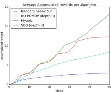
has higher gradient than the top left one. . . 45 3.3 Accumulated rewards for second experiment. . . 45 3.4 Drone flying over a hilly terrain in gazebo simulator. The houses in the

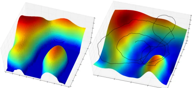
background are used for PTAM positioning. . . 47 3.5 Surface reconstruction after simulated experiment with BO-POMDP

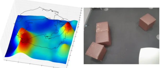
depth 3 (right), trajectory is displayed in black. Ground truth of the hilly terrain (left), as shown in Figure 3.4. . . 48 3.6 Quad-copter used for real-world experiments. . . 49 3.7 Surface reconstruction after real-world experiment with BO-POMDP

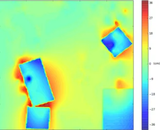
depth 3 (left), trajectory displayed in black. Photo of the corresponding 3×3 meter experiment area (right). . . 49 3.8 Centred surface reconstruction error. A GP with Exponential kernel

was used to reconstruct the map from flight data. The highest error is achieved around prop edges. . . 50

(14)

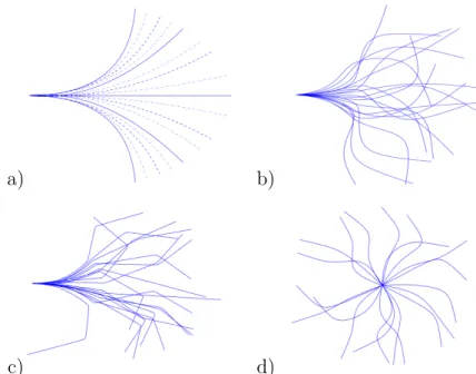
4.1 Picking data points used to construct trajectories in RKHS. This example uses 4 anchor points (including the stating point) and only requires 3 parameters θ0, θ1, θ2. Times yi are evenly distributed between 0 and 1. 64 4.2 Trajectories generated with discrete cubic splines (a). Plain splines are

used for experiments with 5 actions, plain and dashed for 9 actions, dot-ted splines are added to form 17 actions. Kernel trajectories with smooth (b, d) and sharp (c) space kernel kx. The starting angle restriction is

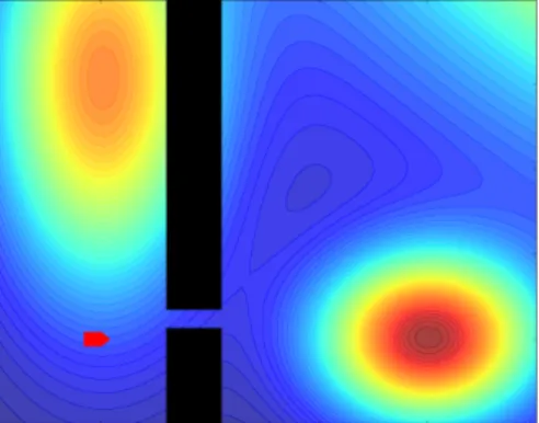
relaxed to allow different types of motion (d). . . 64 4.3 Space modelling domain. Black rectangles are obstacles, the red polygon

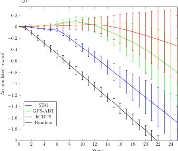
represents the robot’s starting pose, and the background colours show the monitored function (ground truth). High values are red, low values are blue. . . 66 4.4 Mean and standard deviation of accumulated rewards in the space

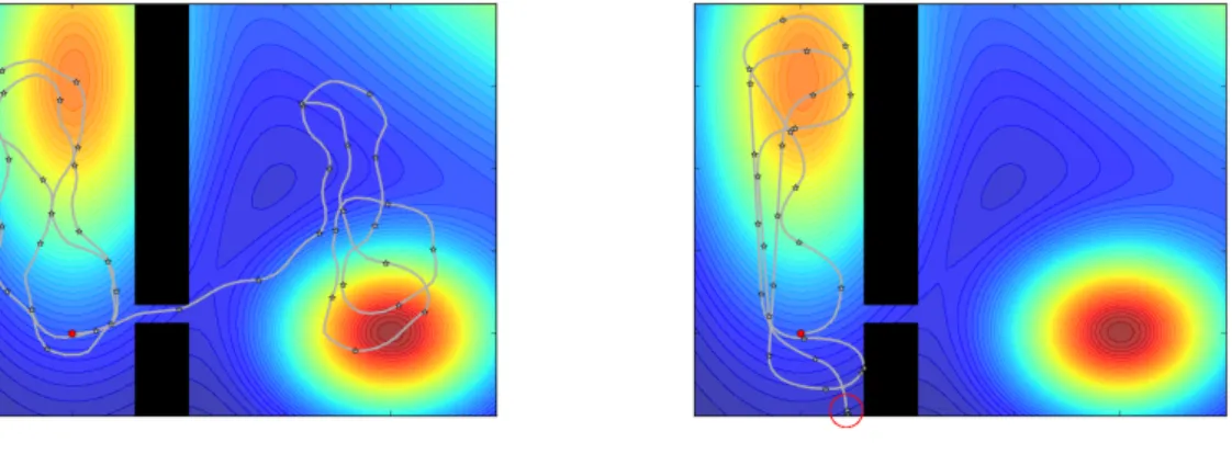
modelling problem, averaged over 200 runs. . . 68 4.5 Example of robot trajectories when using kCBTS (left) and SBO (right).

With kCBTS, the robot manages to navigate through the wall gap. The red circle on the right figure denotes a collision. . . 69 4.6 Accumulated rewards in the simulated robot parking problem, averaged

over 200 runs. . . 72 4.7 Platform used in robot parking problem. . . 73 4.8 Accumulated rewards for five runs (plain) and mean (dashed) in the

robot parking problem. . . 74 5.1 Left: classic intrinsic exploration setup as proposed in [14]. Right:

(15)

List of figures xv

5.2 Mean and standard deviation of returns on cliff walking domain with goal-only rewards. ϵ-greedy exploration achieves near-zero return on most experiments, showing its inability to reach remote states with non-zero reward. (a) Stopping exploration after 30 episodes. (b) Stopping exploration after 30 episodes and continuing exploration after another 10 episodes. (c) Stochastic transitions with 0.1 probability of random action. (d) Rewards are scaled by 100, and exploration parameters are also scaled to keep a equal magnitude between exploration and exploitation terms. . . 92 5.3 Decreasing exploration parameter over time to control exploration level

on sparse CliffWalking (top) and sparse Taxi (bottom) domains. Results are averaged over 100 runs. . . 94 5.4 Taxi domain with goal-only rewards. Top: exploration stops after a

fixed budget is exhausted. Bottom: exploration stops after a test target return of 0.1 is reached on 5 consecutive runs. Results averaged over 100 runs. . . 96 5.5 Return mean and standard deviation for Q-learning with random Fourier

features (RFF) or Fourier basis features on SinglePendulum (top), Moun-tainCar (middle), and DoublePendulum (botom) domain with classic rewards. Results are computed using classic Q-learning with ϵ-greedy policy, and averaged over 20 runs for each method. . . 102 5.6 (a) Chain domain described in [62]. (b) Steps to goal (mean and standard

deviation) in chain domain, for increasing chain lengths, averaged over 30 runs. (c) Steps to goal in semi-sparse 10-state chain, as a function of reward sparsity, with maximum of 1000 steps (averaged over 100 runs). 104 5.7 Goal-only MountainCar. (a,b,c) Exploration value functionU (for action

0) after 1, 2, and 3 episodes. State trajectories for 3 episodes are plain lines (yellow, black and white respectively). (d) Steps to goal (x >0.9), with policy refined after goal state was found (averaged over 30 runs). . 105

(16)

5.8 (a) Manipulator task: learning to reach a randomly located target (red ball). (b) EMU-Q’s directed exploration yields higher performance on this task compared to RFF-Q withϵ-greedy exploration. . . 110

(17)

List of tables

3.1 Reconstruction error for second experiment. . . 47 4.1 Errors on Final Model Reconstruction. . . 70 5.1 Stopping exploration after a target test return of 0.1 is reached on 5

consecutive episodes in Taxi domain. Results averaged over 100 runs. . 95 5.2 Experimental parameters for all 7 domains . . . 108 5.3 Results for all 7 domains, as success rate of goal finding within 100

episodes and mean (and standard deviation) of number of episodes before goal is found. Success rate rate is more important than number of episodes to goal. Results averaged over 20 runs. DORA was run with discretised actions, and RFF-Q with ϵ-greedy exploration on domains with classic rewards. . . 109

(18)

(19)

List of Algorithms

1 Bayesian Optimisation . . . 20

2 MCTS algorithm for BO-POMDP . . . 41

3 Bayesian Optimisation for action selection . . . 59

4 Kernel CBTS (kCBTS) . . . 61

5 Explicit Exploration-Exploitation . . . 90

(20)

(21)

Nomenclature

General Symbol Format

y Unidimensional Variable

y Multidimensional Variable, Vector

Y Matrix

General

P(A) Probability of event A

P(A|B) Probability of event A given event B

f(x) Function over x I Identity Matrix A−1 Matrix inversion A⊤ Matrix transpose |A| Determinant of matrix A xi i th element of vector x

(22)

Linear Regression

x Input in RD

X Matrix of all inputs

t Target in R

t Vector of all targets

N Number of data points

D Dimension of input

D Dataset of composed of N input-target pairs

w Linear regression weights

ϕ(x) Features map for input x, in _RM

Φ Design matrix of size M ×M, with feature maps of all data points

M Number of features

Bayesian Learning

ϵ Zero mean Gaussian noise of precisionβ

β Precision of noiseϵ

wM L Maximum likelihood estimator for linear regression weights α Precision of linear regression weight prior

m Linear regression weight posterior mean S Linear regression weight posterior covariance wM AP Maximum a posteriori for linear regression weights σ2 Bayesian linear regression predictive variance

(23)

List of Algorithms xxiii

Gaussian Process Regression

k Kernel or covariance function

y Modelled function

m Gaussian process prior mean function

θm Prior mean function hyper-parameters

θk Kernel hyper-parameters

σf Kernel variance hyper-parameter

L Kernel covariance hyper-parameters

θ All hyper-parameters

X∗ Matrix of all query inputs

y∗ Vector of all predicted function evaluations

KX Gaussian process Gramm matrix

Sparse Approximation of Gaussian Processes

τ Input of shift-invariant kernel

µ Measure of density p(ω)

ω Random Fourier feature frequencies

Bayesian Optimisation

y Objective function

h Acquisition function

x+ Best known input

µ GP predictive mean function

σ GP predictive standard deviation function

(24)

Reinforcement Learning

S Set or space of states

s State

A Set or space of actions

a Action

R Reward function

r Reward

re Exploration reward

T Transition function

Ω Set or space of observations

o Observation

γ Discount factor

π Policy

π∗ Optimal policy

(25)

List of Algorithms xxv

Abbreviations

BLR Bayesian Linear Regression

BO Bayesian Optimisation

CBTS Continuous Belief Tree Search

CDF Cumulative Density Function

EM Environmental Monitoring

EMU-Q Exploration by Minimising Uncertainty of Q values

FTS Full Tree Search

GP Gaussian Process

GPR Gaussian Process Regression

IEM Environmental Monitoring

LR Linear Regression

MCTS Monte Carlo Tree Search

MDP Markov Decision Process

NLML Negative Log Marginal Likelihood

NLPP Negative Log Predictive Probability

PDF Probability Density Function

PI Probability of Improvement

POMDP Partially Observable Markov Decision Process

RFF Random Fourier Features

RL Reinforcement Learning

RMSE Root Mean Squared Error

SBO Sequential Bayesian Optimisation

UAV Unmanned Aerial Vehicle

UCB Upper Confidence Bound

UCT Upper Confidence Bound for Trees

(26)

(27)

Published Papers

This thesis is based on the work published in the following papers:

Philippe Morere, Román Marchant, and Fabio Ramos. Sequential Bayesian optimisa-tion as a POMDP for environment monitoring with UAVs. InInternational Conference on Robotics and Automation (ICRA), 2017

Philippe Morere, Román Marchant, and Fabio Ramos. Continuous state-action-observation POMDPs for trajectory planning with Bayesian optimisation. In In-ternational Conference on Intelligent Robots and Systems (IROS), 2018

Philippe Morere and Fabio Ramos. Bayesian RL for goal-only rewards. In Conference on Robot Learning (CoRL), 2018

(28)

(29)

Chapter 1 Introduction

1.1 Motivation

Decision making is a major challenge to many robotics and artificial intelligence applications. Complex real-world problems often require agents or robots to interact with their environments to achieve a goal. The applications are countless: from self driving cars to portfolio management and medical interventions. At a time when automation is happening faster than ever, decision making is extremely important. Ideal goals include automating work that is a burden to humans, such as repetitive, administrative or physically demanding tasks. Automated decision making could also contribute towards more impartial decisions, hence providing greater harmony in society.

Decision making is typically defined with a clear objective. This can either be to complete a task by obtaining a desired outcome (eg. driving a passenger to a location), or achieving the best possible score for a given problem (eg. maximum surgery success rate). Although these metrics can be extremely difficult to design in practice, decision making methods usually assume experts can generate such goals or score functions.

Even when a task can be clearly defined using goals or scores, it is often unclear how to solve it. Indeed, people often rely on heuristic for solving problems, leading to sub-optimal performance. Additionally, some tasks are too complex for humans to

(30)

perform (eg. flying an aerodynamically unstable aircraft), and algorithms are required to solve these. When making decisions, people can suffer from a variety of biases. Whether emotionally involved, distracted or simply tired, humans are prone to making mistakes. Decision making algorithms are less likely to suffer from such problems and should result in more consistent performance. Rational decision making could also benefit some aspects of society such as the justice system. Lastly, algorithms can take decisions faster than humans, giving them better reflexes in tasks such as driving. All these reasons make it clear there is much to be gained from developing better decision making algorithms.

Numerous machines have been providing us with low forms of automation for centuries. To grow away from this and achieve higher levels of automation, more intelligent systems need to be developed. These systems should be able to automatically figure out what the best decisions are, and ideally learn for themselves. The first ability – figuring out what the best decisions are – allows for more robustness to changing scenarios, as the automated solution to a problem is not rigidly predefined. Robots and intelligent systems can thus adapt to scenarios different to the intended situation. The second ability – that of learning for themselves – gives intelligent agents the capability to dynamically change the solution to a problem, and adapt it as needed. This behaviour is key to human success as a species and is paramount for higher types of automation.

Real world applications are very challenging for decision making algorithms. Execut-ing the same action in the same situation can sometimes have very different outcomes and consequences, due to the underlyingstochastic dynamicsof the real world. Efficient

decision making systems should either learn or take into account such randomness. Moreover, robots sense parts of the world through imperfect sensors, limiting both the amount of information gathered and its quality. This noisy and partial observability of

(31)

1.2 Problem Statement 3

Although decision making algorithms are desirable and have seen numerous recent developments, there still are many challenges standing in the way of their wider application to real world problems.

1.2 Problem Statement

The problem addressed in this thesis is that of achievingefficient non-myopic decision making in continuous spaces by explicitly balancing exploration and exploitation.

Decision making is the focus of both the fields of planning and reinforcement learning, in which and agent or robot must act to complete an objective. Acting can be achieved by learning a reactive policy, a mapping associating a recommended action to each environment state, or by searching over the space of actions and future consequences. Both approaches are challenging and typically require extensive data and/or computational resources.

Additionally, completing objectives sometimes requires sacrificing short-term per-formance in order to achieve better long-term perper-formance. Decision making methods with this characteristic are known as non-myopic, whereas ones that can only achieve

immediate objectives are qualified as myopic. Non-myopic decision making is more

challenging than its myopic counterpart, as long sequences of actions and their perfor-mance need to be evaluated, thereby greatly increasing the search space size. When spaces – and notably actions spaces – are continuous, the problem becomes intractable and approximation techniques need to be used.

Decision making computes optimal behaviours by balancing two key quantities: exploration and exploitation. Exploitation takes advantage of previously acquired information or high performing solutions, whereas exploration focuses on acquiring more informative data or investigating potential solutions. The balance between these quantities can be found in planning when searching over the space of future sequences of actions, or in reinforcement learning when deciding whether to acquire new data to refine underlying models.

(32)

This work focuses on techniques for efficiently balancing exploration and exploitation in the context of non-myopic decision making in continuous spaces. As a common theme, Bayesian optimisation is used to achieve such balance in both planning and reinforcement learning contexts.

1.3 Contributions

The contributions of this thesis are the following:

• Definition of a novel reward function trading off exploration and ex-ploitation of gradients for sequential Bayesian optimisation. Sequential

Bayesian optimisation was first defined by [49] for addressing spatial monitoring problems. Redefining the objective optimised by this algorithm allows for achiev-ing better performance and plannachiev-ing capabilities. This objective is incorporated to both a myopic planner and a planner based on sequential Bayesian optimisa-tion. Simulation results on the new algorithm, called BO-POMDP, show that this new objective definition leads to performance superior to previous methods. A comparison between the myopic and non-myopic algorithms suggests planning with higher horizons improves monitoring behaviour.

• First practical results of the BO-POMDP formulation on a robotic platform. The proposed method is adapted to a real robotic problem, featuring

a cheap quad-copter which needs to monitor a real environmental variable. The method presented in this work is shown to successfully map terrains, while only using limited sensing capabilities.

• An extension of tree search based planner BO-POMDP to continuous action spaces. BO-POMDP is based on Monte Carlo tree search, which is only

defined for discrete action spaces. This work presents Continuous belief tree search (CBTS), which relies on dynamic action sampling to allow planning on continuous action spaces. Because dynamic sampling favours promising regions

(33)

1.3 Contributions 5

of the action space, it allows finding and selecting more precise actions than traditional sampling techniques, consequently yielding better policies.

• A kernel-based trajectory generation method. This trajectory generation

technique is based of the theory of reproducing kernel Hilbert spaces, allowing it to generate plausible trajectories. As opposed to splines, trajectories can be generated from any set of continuous parameters, making them suited to using the output of an optimisation algorithm. Trajectories display consistent properties such as smoothness and differentiability, which are enforced by kernel functions. These properties are often desired when generating realistic trajectories for real world robotics.

• Evaluation of continuous action planner with kernel trajectories on simulated and real-world experiments. Continuous action planner CBTS

and the proposed kernel trajectory generation technique are complementary; they are combined into a trajectory planner called kCBTS which is validated on simulated and real robotics systems. kCBTS is first applied to a space modelling problem in which a robot learns an objective function by gathering noisy measurements along continuous trajectories. kCBTS is then used to solve a simulated parking problem, in which a robot must manoeuvre to a park with restricted steering angle. Lastly, kCBTS is employed on a real-world robotics problem analogous to the previous parking task, validating the practical applicability of kernel trajectories. Experiments show the proposed method outperforms other existing trajectory planners, while confirming that planning with continuous actions results in higher accumulated reward than when using a discrete set of actions. Additionally, continuous actions allow for better space coverage, resulting in lower errors in final models of the monitored function. • A multi-objective reinforcement learning framework for explicit

ex-ploration exploitation balance. Exploration and exploitation are distinct

(34)

ex-ploitation and treat exploration in an ad-hoc manner. A framework separating these two quantities is proposed, based on the theory behind multi-objective reinforcement learning. By modelling exploration and exploitation separately, their balance can be brought at a policy level, making it core to the optimisation problem.

• Experimental evaluation of the framework with classic exploration strategies. The proposed framework for explicit exploration-exploitation balance

is experimentally evaluated against classic exploration strategies such as intrinsic RL exploration bonuses. Results demonstrate separating both exploration and exploitation signals and treating them as distinct objectives is beneficial to learning and several key exploration characteristics.

• Strategies for online exploration-exploitation balance tuning. Drawing

inspiration from the fields of bandits and Bayesian optimisation, strategies to tune the exploration-exploitation balance online can be devised. These strategies achieve a degree of control over agent exploration that was previously unattainable with classic additive intrinsic rewards. Also, the additional flexibility is beneficial to more practical application such as robotics.

• A data-efficient model-free RL method based on the explicit exploration-exploitation balance framework. A method based on the previous framework

is proposed, displaying scalability to larger problems. The method, termed EMU-Q, guides exploration to areas of the state-action space with high value function uncertainty. The algorithm builds on sparse Gaussian process approximation techniques, thereby allowing larger problems with more data to be addressed, and is optimised for online learning.

• EMU-Q is experimentally shown to outperform other exploration tech-niques. EMU-Q is evaluated on a large benchmark of reinforcement learning

(35)

1.4 Thesis Outline 7

favourably against classic exploration techniques and more advanced methods such as intrinsic RL with additive rewards.

1.4 Thesis Outline

An overview of the chapters presented in this thesis is given below.

Chapter 2: Theoretical Background

The main concepts used in this work are presented in this chapter. These include regression methods such as Gaussian processes andBayesian linear regression, used to

model various functions of interest. Optimisation techniques allowing robots to act near-optimally are also described. These include Bayesian optimisation for finding

sampling locations and reinforcement learning methods for learning policies.

Chapter 3: Bayesian Optimisation for Sequential Planning

This chapter describes a method for using Bayesian optimisation as a sequential planner. The problem of sequential continuous planning is first presented, and a myopic method relying on Bayesian optimisation is given. A new formulation based on partially observable Markov decision processes is presented to allow non-myopic planning, and is solved using Monte Carlo tree search. Experiments on simulated problems and real-word robotic scenarios are displayed, demonstrating the benefits of the approach.

Chapter 4: Sequential Planning with Continuous Actions

The problem of sequential planning is extended to scenarios with continuous actions in this chapter. Belief tree search, a variant of Monte Carlo tree search, is described to illustrate the limitation of tree search based planners to discrete action spaces. Continuous belief tree search is proposed as an extension of belief tree search to continuous action spaces by using Bayesian optimisation to sample actions within the tree search. Kernel trajectories are then proposed as a trajectory generation technique,

(36)

designed to work with optimised and continuous action parameters. Kernel trajectories complement the proposed planner and are combined into a stand-alone algorithm. Experiments demonstrate the superiority of the approach compared to planners with discrete actions, on both simulated and real-world robotic problems.

Chapter 5: Bayesian Optimisation for Reinforcement Learning

This chapter relaxes the assumption of known dynamics and reward function used in previous chapters by casting the problem of interest into the reinforcement learning framework. The exploration-exploitation balance problem of reinforcement learning is first described from an intrinsic and multi-objective RL perspective. A solution for making this balance explicit is given, defining a model-free RL framework inspired by Bayesian optimisation. Techniques for taking advantage of the explicit balance are then described, yielding significant practical advantages on simple examples. A concrete algorithm for achieving efficient exploration in RL is then proposed, where exploration is carried by minimising the uncertainty of the state-action value function. The framework and algorithm are validated on synthetic domains, benchmark RL environments, and a realistic robotic simulator. The method shows enhanced exploration speed and data-efficiency compared to other exploration methods.

Chapter 6: Conclusions and Future Work

Conclusions of the work presented in this thesis are drawn in this chapter. Contributions are then summarised, and avenues for future work are finally proposed as promising directions for future research.

(37)

Chapter 2 Theoretical Background

2.1 Introduction

This chapter provides background for understanding and developing the techniques presented in this thesis. Decision making algorithms rely on learning diverse models. For example: planning algorithms typically require to maintain a belief, which can be represented as a probabilistic model; and model-free reinforcement learning methods rely on learning a state-action value function, which reduces to a regression problem. This first few sections of this chapter provide relevant background on regression and probabilistic model learning such as linear regression (LR) in Section 2.2, Bayesian linear regression (BLR) in Section 2.4, Gaussian processes (GP) and a sparse GP

approximation in Sections 2.5 and 2.6.

The solutions presented in this work explicitly balance exploration and exploitation to improve decision making algorithms. Section 2.7 presents Bayesian optimisation

(BO), a search and optimisation technique based on this principle. BO is one of the key algorithms this work builds on.

Non-myopic decision making requires reasoning about long-term consequences of actions to guarantee optimal behaviours can be found. This long-term reasoning is typically formulated using the well-studied frameworks of Markov decision processes

(38)

described in Section 2.8. Lastly, an overview of reinforcement learning is given in Section 2.9.

2.2 Linear Regression

Regression is a category of supervised learning where the goal is to predict values in a continuous domain. Regression typically consists of learning a continuous function mapping inputs x to a continuous (potentially multi-dimensional) target t. Such function, also called model, is generally parametrised by a vector of parameters whose value can be estimated from historical data. The problem of regression can then be formulated as finding the best value or distribution of model parameters, given a datasetD = (X,t) ={xn, tn}Nn=1 ofN input-target pairs (x, t). The target variable is

typically assumed to be given by a deterministic function y of the input and model parameters and perturbed by Gaussian noise

tn=yn(w,xn) +ϵ, (2.1)

where ϵ is a zero mean Gaussian random variable of precision β.

Linear regression (LR) is the simplest regression model, predicting targets as a linear combination of inputs:

yn(w,xn) = w0 +w1x1n+...+wDxDn, (2.2) where xn= [x1n, ..., xnD] and w = [w0, ...wD] are the model parameters or weights. This

model learns linear mapping of inputs, greatly restricting its expressive power.

This model can easily be extended to using features, allowing for learning mappings

linear in the features and typically non-linear in the inputs: yn(w,xn) =w0+

M−1

X

j=1

(39)

2.2 Linear Regression 11

A set of M −1 features ϕ(x) = {ϕj(x)}Mj=1−1 are defined as functions of the input.

Defining a additional bias featureϕ0 = 1, the model can be rewritten more compactly

yn(w,xn) =

M−1

X

j=0

wjϕj(xn) =w⊤ϕ(xn). (2.4) Defining expressive feature maps has been an active field of research and many definitions were proposed. Polynomial features take the form of powers of the input, such asϕj(x) = xj, allowing the linear regression model to learn a polynomial mapping between inputs and targets. Another kind of features proposes dividing the input space into regions where different local functions are used in each region. These local functions include (but are not restricted to) polynomials, splines, and radial basis functions. More recently, features local in the spectral space of inputs were proposed, called random Fourier features. Background on these features is covered in Section 2.6.1.

Solving a linear regression problem reduces to finding an estimate of model param-eters w. A classic estimator is one which minimises the mean square error (MSE) of

training predictions, formally defined as ˆ w= arg min w N X n=1 (tn−w⊤ϕ(xn))2. (2.5) A closed-form solution for ˆw can be derived by differentiating the MSE and setting it

to zero: 0 = XN n=1 (tn−wˆ⊤ϕ(xn))ϕ(xn)⊤ (2.6) 0 = XN n=1 tnϕ(xn)⊤−wˆ⊤ N X n=1 ϕ(xn)ϕ(xn)⊤ (2.7) ˆ w= (Φ⊤Φ)−1Φ⊤t. (2.8)

Here Φis the N ×M design matrix whose elements are given by Φnj =ϕj(xn). The last equation is known as the standard equation for least-squares linear regression.

(40)

2.3 Bayesian Learning

The linear regression formulation introduced in the last section finds model parameter estimates by minimising a loss function, the MLE. Alternatively, the problem can be reformulated in a way fitting the Bayesian learning methodology more closely. The target variable is assumed to be given by a deterministic function of the input and model parameters and perturbed by Gaussian noise as shown in Equation 2.1. This relationship can also be expressed as with the following conditional, where a linear model with features is used:

p(tn|w,xn, β) = N(tn|w⊤ϕ(xn), β−1). (2.9) The likelihood function can then be defined as

p(t|w,X, β) = N

Y

n=1

N(tn|w⊤ϕ(xn), β−1), (2.10) where the product of conditionals translates the implicit assumption of independence between data points. Note that finding the estimator that maximises Equation 2.10 is equivalent to the estimator derived in Equation 2.8, also referred to as maximum likelihood estimator orwM L.

However, in the Bayesian learning methodology, model parameters are typically treated as random variables, for which prior distributions are defined. This allows for deriving estimators or model parameter posterior distributions by making use of Bayes’ rule, hence mixing prior information with likelihood information in a natural way.

In the simplest case, a Gaussian isotropic prior can be defined for model parameters

w such that

(41)

2.4 Bayesian Linear Regression 13

with prior precision parameter α. Using Bayes’ rule and the likelihood defined in Equation 2.10, the model parameter posterior distribution p(w|t,X) can be written as

p(w|t,X;α, β) = p(t|w,X;β)p(w;α)

p(t;α, β) , (2.12)

wherep(t;α, β) is the evidence ormarginal likelihood function.

Because both the likelihood function and the model parameter prior were chosen to be Gaussian distributions, the posterior distribution is also Gaussian and can be computed in closed-form. The expression for the model parameter posterior distribution can be derived by expanding prior and likelihood expressions and completing the square in a tedious but straight-forward process [8], leading to

p(w|t,X;α, β) =N(w|m,S), (2.13)

where m=βSΦ⊤t, (2.14)

S = (αI +βΦ⊤Φ)−1. (2.15) A new model parameter estimator can be derived, by seeking to maximise the the posterior distribution. This estimator is referred to as maximum a posteriori (MAP) or

wM AP, and is given by Equation 2.14 as the mode and mean of Gaussian distributions coincide. This estimator differs from the maximum likelihood estimator in that prior information is incorporated and controlled by hyper-parameter α. Asα tends to zero, the prior becomes infinitely broad and uninformative, and the expression for wM AP is identical to that of wM L.

2.4 Bayesian Linear Regression

Instead of deriving parameter estimators, the quantity of interest in Bayesian linear regression (BLR) is the full parameter posterior distribution. Incorporating the full distribution when making predictions results in more information available than with

(42)

maximum likelihood or maximum a posteriori method, as several parameter posterior distribution moments can often be computed.

Following the same derivation as for the maximum a posteriori estimator, the model parameter posterior is given by Equation 2.13. When making predictions, the Bayesian linear regression model makes use of the whole model parameter posterior distribution; the predictive distribution p(t|x,t, α, β) for a new point x is computed as follows by

marginalising over model parameters: p(t|x,t,X;α, β) =

Z

p(t|w,x;β)p(w|t,X;α, β)dw (2.16)

=N(t|m⊤ϕ(x), σ2(x)), (2.17) where the predictive variance σ2(x) is given by

σ2(x) = β−1+ϕ(x)⊤Sϕ(x). (2.18) Contrary to linear regression, Bayesian linear regression provides predictive variance information which can be used to assess prediction confidence. The predictive variance in Equation 2.18 is composed of two terms: the first one represents data noise whereas the second one encodes the uncertainty associated with model parameters w.

One of the advantages of working with model parameter priors and posteriors is that the Bayesian linear regression model can seamlessly be updated in closed-form, in light of new data. The update procedure involves replacing the current prior (of mean

mi−1 and covariance Si−1) by the current posterior (of mean mi and covariance Si) and applying Bayes’ rule once again with the likelihood of the new data to compute the new posterior (of mean mi+1 and covarianceSi+1). Formally, the model parameter

prior is defined as

(43)

2.5 Gaussian Process (GP) Regression 15

and the posterior distribution is

p(w|t,X;α, β) =N(w|mi+1,Si+1), (2.20)

where mi+1 =Si+1(Si−1mi+βΦ⊤t), (2.21)

Si+1 = (Si+βΦ⊤Φ)−1. (2.22) These equations can be used to cheaply update the posterior iteratively, as new data is made available.

Lastly, hyper-parametersα and β can be optimised by minimising the negative log marginal likelihood (NLML) −lnp(t|α, β). Rearranging Equation 2.12, the NLML can be written as follows: −lnp(t|α, β) = E(m) + 1 2ln|S −1_|₊ N 2 ln(2π)− M 2 ln(α)− N 2 ln(β), (2.23) where E(m) = β 2||t−Φm||2+ α 2m ⊤ m. (2.24)

When minimising the NLML, values of α and β are learned from data only (no prior was used for either hyper-parameterαor β), and their estimate is referred to as type-II maximum likelihood. Note that feature parameters, which have been omitted thus far, can also be optimised using the NLML. This procedure is however expensive as it requires training the model anew at each iteration of the NLML minimisation process.

2.5 Gaussian Process (GP) Regression

Gaussian processes (GP) provide a more expressive Bayesian regression framework, not limited to representing linear trends. A Gaussian process places a probability distribution over functions y, defined as a multivariate Gaussian distribution. The space of possible functions fitting the dataset is fully characterised by a meanm(x|θm)

(44)

two input vectors. The Gaussian process model is written as

y(x)∼ GP(m(x|θm), k(x,x′|θk)), (2.25) where θm and θk are mean and covariance hyper-parameters respectively.

Gaussian process regression gives a predictive distribution where mean and variance are function of the inputx. The mean function is generally assumed to be zero, i.e.,

m(x) = 0. Conversely, the choice of kernel greatly impacts the type of functions that

can be modelled, and is the subject of much work. The most common choice is the square exponential kernel, given by

k(x,x′) =σ_f2exp((x−x

′₎⊤_L₍_x₋_x′₎

2 ), (2.26)

where L is a square matrix of size D, typically chosen as a diagonal matrix containing length-scale parameters for each of the dimensions of the data: L(i,j)= 1/l2i. Both σ2f and the elements of L are considered kernel hyper-parameters and grouped intoθk.

Regression with Gaussian processes involves solving the problem of posterior infer-ence, and potentially learning hyper-parametersθm andθk. A datasetD ={xn, tn}Nn=1

is composed of noisy data from y such that t =y(x) +ϵ, where ϵ is Gaussian noise ϵ∼ N(0, σ_{n). The posterior joint distribution of observed values}2 _t_{and predicted values} y∗ at query points X∗ is given by

   t y∗   ∼ N  0,    K(X,X) +σ2 nI K(X,X ∗₎ K(X,X∗)⊤ K(X∗,X∗)     , (2.27)

where X and X∗ are training and testing inputs respectively and K(·,·) are matrices such that K(X′,X′′)(i,j)=k(Xi′,X

′′

(45)

2.6 Sparse Approximation of Gaussian Processes 17

The predictive distribution at testing locationsp(y∗|X∗,y,X) is a Gaussian

distri-bution with mean and covariance given by

E[y∗|X∗,y,X] =K(X∗,X)[K(X,X) +σn2I]

−1₍_t₋_M₍_X₎₎ _(2.28)

Cov[y∗|X∗,y,X] =K(X∗,X∗)−K(X∗,X)[K(X,X) +σ2_nI]−1K(X,X∗), (2.29) whereM(·) is a mean vector such that M(X)(i) =m(Xi).

Learning the hyper-parameters of a Gaussian process follows a similar procedure to the one described for Bayesian linear regression. All model hyper-parameters are grouped into a vector θ. The simplest approach to estimating a good set of

hyper-parameters is by maximising the log likelihood function. In the case of Gaussian process regression, this function takes the following form:

logp(t|θ) = −1 2log|KX| − 1 2t ⊤ K_X−1t− N 2 log(2π), (2.30) whereKX =K(X,X) +σ2nI.

2.6 Sparse Approximation of Gaussian Processes

Gaussian processes provide a powerful tool for non-linear regression. However, both the inference and learning phase require inverting matrix KX of size N ×N, which becomes prohibitively expensive when N is moderately high. Much Gaussian process literature is dedicated to proposing approximations, which provides slightly worse regression performance to the full model at a fraction of the computational cost. These methods are often based on finding a representative set of M << N inducing points to summarise the dataset, resulting in a much smaller matrix KX to invert. A review of Gaussian process approximation techniques in given in [68].

Another approach approximates the kernel function used to construct KX with a set of M features. These features can be be directly plugged into a Bayesian linear regression model to approximate a Gaussian process. This method, described in the

(46)

next section, is in often easier to use and more flexible than other approximation techniques based on learning a representative set of inducing points.

2.6.1 Random Fourier Features

This section describes random Fourier features (RFF) [69], a technique which allows linear models to enjoy the expressivity of kernel methods by providing features ap-proximating kernels. It should be noted that these features are different from Fourier basis [34], which do not approximate kernel functions.

For any shift invariant kernel, which can be written as k(τ) with τ = x−x′,

a representation based on the Fourier transform can be computed with Bochner’s theorem [23].

Theorem 1 (Bochner’s Theorem) Any shift invariant kernel k(τ), τ ∈ _RD_{, with a}

positive finite measure dµ(ω) can be represented in terms of its Fourier transform as

k(τ) =

Z RD

e−iωτdµ(ω). (2.31)

Assuming measure µ has a densityp(ω), p is the spectral density ofk and we have k(τ) = Z RD e−iτωp(ω)dω≈ 1 M M X j=1 e−iτωj =_⟨_ϕ(_x)_,_ϕ(_x′)_⟩, (2.32)

where p is the spectral density ofk, ϕ(x) is an approximate feature map, and M the number of spectral samples fromp. In practice, the feature map approximatingk(x,x′)

is

ϕ(x) = √1

M[cos(x

⊤

ω1), ...,cos(x⊤ωM),sin(x⊤ω1), ...,sin(x⊤ωM)], (2.33) where the imaginary part was set to zero, as required for real kernels. In the case of the radial basis function kernel defined as k(x,x′) = exp(−0.5σ−2||x−x′||2

2), the

kernel spectral density is Gaussian p=N(0,2σ−2_I_{). Feature maps can be computed}

by drawing M

2 ×d samples fromp one time only, and computing Equation 2.33 on new

(47)

2.7 Bayesian Optimisation 19

kernel function, which should be chosen to represent adequate distance measures for the problem of interest. Correspondence tables between numerous kernels and their spectral densities are given in [69].

2.6.2 Approximate GP with Bayesian Linear Regression

As the number of random Fourier features increases, kernel approximation error decreases [85]. In the limit of an infinite number of features the exact kernel can be recovered from the feature map, and linear regression with this feature map is equivalent to kernel regression. Combining random Fourier features with Bayesian linear regression is very closely related to Gaussian process regression, as detailed in [42]. This approximate Gaussian process model has the same complexity as Bayesian linear regression, which scales with the number of features M, and does not suffer from the high complexity of Gaussian processes which depends on N.

Further reduction of complexity with this approximate GP can be achieved by reducing the number of features used. One solution relies on sampling frequencies according to a quasi-random sampling scheme, reducing kernel approximation error compared to classic Monte Carlo sampling with the same number of features [94].

2.7 Bayesian Optimisation

Bayesian optimisation (BO) is a technique aiming to find the optimum x∗ ∈_RD _{of an} objective function y:_RD _→

Rby gathering noisy observations from it. Formally, x∗ = arg max

x y(x) (2.34)

Noisy observations are assumed to result from an additive Gaussian noise on the function evaluation. The ith observation is defined as ti = y(xi) +ϵ, where ϵiid∼ N(0, β−1) is the noise associated with each independent observation. Extensive theory on BO can be found in [11]. Most implementations of BO use Gaussian processes to model

(48)

the objective function f, although any other probabilistic model can be used. The GP model is updated with a data couple (xi, ti) every time a noisy observation ti is made at location xi. The search of where to get an observation next is guided

by an acquisition function h. At each iteration in the BO algorithm, the location at which to evaluate y is determined by finding arg maxxh(x), therefore reporting

the maximisation problem fromy to h. h is much easier to optimise with traditional techniques such as DIRECT [28] and, is typically much cheaper and faster than y to evaluate. An implementation of BO is detailed in Algorithm 1.

Algorithm 1 Bayesian Optimisation

1: Letxi be the sampling point at iteration i.

2: LetD ={(x1, t1), ...,(xn, tn)} be the data.

3: Leth be an acquisition function.

4: for i= 1,2, .., n do

5: Find xi = arg maxxh(x|D1:i−1).

6: Sample the objective function tt =y(xi) +ϵi.

7: Augment the data D_1:_i ={D_1:_i−1,(xi, ti)}.

8: Recompute the GP model with D1:i.

9: end for

2.7.1 Acquisition Function for Bayesian Optimisation

Acquisition functions are designed to guide the search for better sampling locations in Bayesian optimisation. Hence it is crucial to select a good acquisition function to achieve better performance and sample efficiency. Typically, acquisition functions are designed to reflect the probability of the objective function being high at a given location. This probability can be estimated using full posterior information from the probabilistic model learned in BO. Many popular acquisition functions exist; Probability of Improvement and Upper Confidence Bound are presented here.

(49)

2.8 Sequential decision making 21

Probability of Improvement

The probability of improvement (PI) acquisition function described in [38] computes the probability that sampling at a new input location improves over the best known location x+_{= arg max}

xi∈Xy(xi). Formally, P I(x)_≜p(y(x)≤y(x+) +ξ) (2.35) =Φµ(x)−y(x+)−ξ σx , (2.36)

where Φ is the Gaussian distribution CDF,µandσare the posterior mean and standard deviation of the probabilistic model learned by BO, and ξ≤0 is a parameter trading off exploration and exploitation.

Upper Confidence Bound

The upper confidence bound (UCB) acquisition function described in [16] is often used for its simplicity and ease of use. It only considers the mean and standard deviation of the underlying probabilistic model at a given input location:

U CB(x)_≜µ(x) +κσ(x), (2.37) where κ ≥0 is also an exploration-exploitation trade off parameter. High values of κ result in more exploration around less sampled areas, while lower values favour exploitation near previously sampled locations.

2.8 Sequential decision making

Markov decision processes (MDP) and partially observable Markov decision processes (POMDP) are frameworks used for sequential decision making, notably in the fields of planning and reinforcement learning. Both frameworks define a way to model

(50)

interactions between a learning agent and a dynamical system, making it possible to learn agent behaviours that achieve a desired task.

2.8.1 Markov Decision Process

Agents can interact with anenvironment (ordomain) by takingactionsand can observe

a description of the environment state. Executing an action in a specific state results

in the environment changing states, called transition. Each action taken in a given

state is associated with a reward reflecting how helpful the action is to achieve a goal

task. Agents act according to a policy π, which determines actions to execute in any state of the environment.

Formally, a MDP is defined by the tuple <S,A, T, R, γ >. S and A are spaces of states s and actions a respectively. The transition function T : S × A × S → [0,1] encodes the probability to transition to state s′ when executing action a in state s, i.e. T(s, a, s′) = p(s′|s, a). The reward distribution R of support S × A × S defines the rewardr associated with transition (s, a, s′). The discount factor γ ∈[0,1) diminishes the importance of long-term action consequences. MDPs rely on the Markov assumption, which states the distribution on future states only depends upon the current state, and hence the current state contains all the necessary environment information to act optimally. Solving a MDP is equivalent to finding the optimal policy π∗ starting from s0: π∗ = arg max π ET ,R,π[ ∞ X i=0 γiri], (2.38)

with ai ∼π(si), si+1 ∼T(si, ai,·), and ri ∼R(si, ai, si+1).

2.8.2 Partially Observable Markov Decision Process (POMDP)

POMDPs extend MDPs to decision making under uncertainty [80]. Unlike in Markov decision processes, the agent does not have direct access to the environment state but only receives limited state information via observations. It must instead act relying

(51)

2.8 Sequential decision making 23

for the agent to maintain a probability distribution over the set of possible states. A POMDP is fully defined by the tuple <S,A, T, R,Ω, O, γ >, with:

- S: Set of states {s1, s2, ..., sn}. - A: Set of actions {a1, a2, ..., am}.

- T: S × A × S →[0,1] is a transition function interpreted as the probability to transition to states′ when executing actionain states, i.e. T(s, a, s′) =p(s′|s, a). - R: S × A →_R is a reward function defining the reward of executing actiona in

state s, i.e. R(s, a).

- Ω: Set of observations {o1, o2, ..., ol}.

- O: S × A ×Ω→[0,1] is an observation function that represents the probability of observing o when action a was executed and led to states, i.e. O(o, a, s) = p(o|a, s).

- γ ∈[0,1] is the discount factor.

POMDPs also rely on the Markov assumption, hence it is not necessary to keep track of an observation history as all information at timet is assumed to be embedded in the current belief state bt(s).

Solving a POMDP is equivalent to finding the optimal policy π∗ : Ω → A. The optimal policy is defined as the one maximising the expected infinite sum of discounted rewards rt starting from belief state b0. More formally,

π∗ = arg max π E[ ∞ X t=0 γtr_tπ|bo] (2.39) whererπ

t is the reward given for following policyπ at time t.

Numerous methods to solve MDPs and POMDPs were proposed over the years. Learning policies when transition and/or reward and observation functions are unknown

(52)

falls into the field of reinforcement learning, whereas the task is typically referred to as planning when all functions are known.

2.9 Reinforcement Learning

Reinforcement learning addresses a class of learning problems where an agent interacts with a dynamic, potentially stochastic and partially unknown environment, aiming to learn policies that maximise performance on a given task [87]. The interactions between agent and environment are typically modelled using a Markov decision process when states are observable, or a partially observable Markov decision process in when only limited state information is accessible. Reinforcement learning has received much recent attention, and methods to learn policies from interaction with an environment fall into several families. This section gives an overview and basic theory on the main classes of reinforcement learning methods.

2.9.1 Model-based

The principle behind model-based methods is to learn the MDP’s transition dynamics, and use a planning algorithms to find the best action to execute next. This family of methods is called model-based to reflect the model used to learn transition dynamics.

By opposition, the next two families of RL algorithms do not learn the transition dynamics explicitly and are often referred to asmodel-free RL.

Learning the transition dynamics of an MDP can be cast as a supervised learning problem using transition data collected from interactions between agent and envi-ronment. Transitions are tuples (st, at, st+1), and the state-action pair (st, at) and next state st+1 can be used as input and target of a supervised learning algorithm,

respectively. Some model-based RL algorithms similarly learn the reward function from transition data.

Once the transition function (and possibly reward function) is learned, action selection is reduced to a planning problem. Indeed, when components of the MDP are

(53)

2.9 Reinforcement Learning 25

known, planning algorithms such as full tree search or Monte Carlo tree search can find the optimal action at a given state. In this case, the policy is not a function but a planning algorithm. Examples of model-based RL algorithms include Dyna [86] and prioritised sweeping [53].

Model-based RL methods are known for their high data efficiency, which makes them perfect candidates for real life problems where data is scarce or expensive. Furthermore, these methods can handle changing objectives and tasks (change in rewards), without needing to learn models anew. However, model-based algorithms generally do not scale well with high dimensions, and learning models and planning can be computationally expensive. Lastly, resulting policies are sensitive to compounding transition model errors, and a slightly wrong transition model can result in degenerate policies.

2.9.2 Value function

The core idea of value function RL [13] is to learn a value functionV (or state-action value function Q), which encodes the expected long-term discounted value of a state (or state-action pair):

V(s) =_ET ,R,π[ ∞ X i=0 γiri|s0 =s], (2.40) Q(s, a) =_ET ,R,π[ ∞ X i=0 γiri|s0 =s, a0 =a], (2.41)

whereri =R(si, ai). These functions reflect the expected sum of discounted reward gained from following policy π, starting from s0 = s (and a0 = a in the case of Q).

These value functions are difficult to learn in practice, but have the advantage of making the policy definition simple. Because value functions encode the value of a state (or state-action pair) using an infinite horizon, high horizon action search is not necessary to achieve non-myopic action selection.

(54)

When the state-action value function is optimal, denoted Q∗, the optimal policy simply becomes a maximisation over the action space:

π∗(s) = arg max a∈A Q

∗₍

s, a). (2.42)

Learning the state-action value function can be achieved by writing Equation 2.40 recursively, also known as the Bellman equation:

Q(s, a) =_ER[R(s, a, s′)] +γ_Es′_,a′_|s,a[Q(s′, a′)]. (2.43)

Here, s′ ∼ p(s′|s, a) and a′ ∼ π(s′). This equation can be used to iteratively refine models of Q based on transition data, and is the base of most value function RL algorithms such as Q-learning [90]. In the tabular case, learning Q with Equation 2.43 converges to the optimal state-action value function Q∗, which is used to recover the optimal policy π∗.

Value function methods are generally simple algorithms, of low complexity. Learning is relatively data efficient, while not requiring the computational overhead of learning MDP transition dynamics. However, this family of methods does not scale very well with very high dimensions, and does not provide ways to inspect how much of the environment dynamics the agent has learned. Examples of value function RL include value iteration [6, 87], Q-learning [90], SARSA [75], and least-squares temporal difference [40].

2.9.3 Policy search

Policy search methods take a different approach and directly search over a space of policies to find the best performing one. Policies are modelled as function mapping statess to actionsa and fully defined by a vector of parametersθ. Finding the optimal

Bayesian Optimisation for Planning And Reinforcement Learning

Bayesian Optimisation for Planning

and Reinforcement Learning

Philippe Morere

A thesis submitted in fulfillment

of the requirements of the degree of

Doctor of Philosophy

School of Computer Science

The University of Sydney

Declaration

Bayesian Optimisation for Planning and

Reinforcement Learning

Acknowledgements

Table of contents

List of figures

List of tables

List of Algorithms

Nomenclature

General Symbol Format

General

Linear Regression

Bayesian Learning

Gaussian Process Regression

Sparse Approximation of Gaussian Processes

Bayesian Optimisation

Reinforcement Learning

Abbreviations

Published Papers

Chapter 1

Introduction

1.1

Motivation

1.2

Problem Statement

1.3

Contributions

1.4

Thesis Outline

Chapter 2

Theoretical Background

2.1

Introduction

2.2

Linear Regression

2.3

Bayesian Learning

2.4

Bayesian Linear Regression

2.5

Gaussian Process (GP) Regression

2.6

Sparse Approximation of Gaussian Processes

2.6.1

Random Fourier Features

2.6.2

Approximate GP with Bayesian Linear Regression

2.7

Bayesian Optimisation

2.7.1

Acquisition Function for Bayesian Optimisation

2.8

Sequential decision making

2.8.1

Markov Decision Process

2.8.2

Partially Observable Markov Decision Process (POMDP)

2.9

Reinforcement Learning

2.9.1

Model-based

2.9.2

Value function

2.9.3

Policy search