UNCERTAINTY QUANTIFICATION IN THE CLASSIFICATION OF
HIGH DIMENSIONAL DATA∗
ANDREA L BERTOZZI †, XIYANG LUO ‡, ANDREW M. STUART §, AND
KONSTANTINOS C. ZYGALAKIS ¶
Abstract. Classification of high dimensional data finds wide-ranging applications. In many of these applications equipping the resulting classification with a measure of uncertainty may be as important as the classification itself. In this paper we introduce, develop algorithms for, and investigate the properties of, a variety of Bayesian models for the task of binary classification; via the posterior distribution on the classification labels, these methods automatically give measures of uncertainty. The methods are all based around the graph formulation of semi-supervised learning.
We provide a unified framework which brings together a variety of methods which have been introduced in different communities within the mathematical sciences. We study probit classification [43], generalize the level-set method for Bayesian inverse problems [24] to the classification setting, and generalize the Ginzburg-Landau optimization-based classifier [5,40] to a Bayesian setting; we also show that the probit and level set approaches are natural relaxations of the harmonic function approach introduced in [49]. We introduce efficient numerical methods, suited to large data-sets, for both MCMC-based sampling as well as gradient-based MAP estimation. Through numerical experiments we study classification accuracy and uncertainty quantification for our models; these experiments showcase a suite of datasets commonly used to evaluate graph-based semi-supervised learning algorithms.
Key words. Graph classification, Uncertainty quantification, Gaussian prior
AMS subject classifications. 6209, 65S05, 9404
1. Introduction.
1.1. The Central Idea. Semi-supervised learning has attracted the attention of many researchers because of the importance of combining unlabeled data with labeled data. In many applications the number of unlabeled data points is so large that labeling training data is expensive and time-consuming. Therefore, the problem of effectively utilizing a combination of unlabeled and labeled information is very important in machine learning research. This paper concerns the issue of how to address uncertainty quantification in such classification methods. In doing so we bring together a variety of themes from the mathematical sciences, including optimization, PDEs, probability and statistics. We will show that a variety of different methods, arising in very distinct communities, can all be formulated around a common objective function
J(w) =1
2hw, P wi+ Φ(w) ∗Submitted to the editors DATE.
Funding: NSF grant DMS-1118971, NSF grant DMS-1417674, and ONR grant N00014-16-1-2119. AMS is funded by DARPA and EPSRC. KCZ was partially supported by a grant from the Simons Foundation and by the Alan Turing Institute under the EPSRC grant EP/N510129/1. Part of this work was done during the author’s stay at the Newton Institute for the program Stochastic Dynamical Systems in Biology: Numerical Methods and Applications.
†Department of Mathematics, University of California Los Angeles, Los Angeles, CA ([email protected]).
‡Department of Mathematics, University of California Los Angeles, Los Angeles, CA (
§Computing and Mathematical Sciences, Caltech, Pasadena, CA ([email protected]). ¶School of Mathematics, University of Edinburgh, Edinburgh, Scotland ([email protected]).
1
for a real valued functionwon the nodes of a graph representing the data points. The matrixP is proportional to a graph Laplacian derived from the unlabeled data and the function Φ involves the labelled data. The variable w is used for classification. Minimizing this objective function is one approach to such a classification. A prob-ability distribution related to the objective function has density P(w) proportional to exp −J(w); probability of the labelling variable w is high where the objective function is small, and vice-versa. Uncertainty quantification corresponds to using the probability distribution to compute expectations of test functions g, defined on the nodes of the graph, which enable us to measure the variability of label variables, such as means and variances:
Z
g(w)P(w)dw.
In the settings of interest this will typically be a very high dimensional integral, with the dimension given by the number of unlabelled data points. Carrying out this program requires computational algorithms to minimize J(w) or to draw samples, via Monte Carlo Markov chain (MCMC) for example, from the probability distribu-tion with densityP(w). These algorithms exploit the fact that 12hw, P wiis a graph
analogue of the Dirichlet energy and will leverage analogies with PDE-based method-ologies involving the classical Euclidean Dirichlet energy in order to derive effective computational methods. In this paper we will describe this confluence of ideas from different parts of the mathematical sciences, show how our approach builds on a broad range of advances in the field which we will review, and demonstrate the emergence of a problem area with many open challenges for the mathematical sciences. We em-phasize that the variety of probablistic models considered in this paper arise from different assumptions concerning the structure of the data. Our objective is not to as-sess the validity of these assumptions, which is a modelling question best addressed on a case-by-case basis, but rather we develop an overarching computational framework suitable for all the models arising from these different assumptions.
1.2. Literature Review. An effective method for semi-supervised learning is to construct a similarity graph on both the unlabeled and labeled examples, and clas-sify unknown labels by leveraging the graph structure. A central conceptual issue in the setting of this problem is that labels are discrete, whilst similarity information is often continuous. Strategies to work with both of these settings simultaneously are at the heart of this subject. In [8], Blum et al. posed the binary semi-supervised clas-sification problem using a graph min-cut problem. This is equivalent to a maximum a posteriori (MAP) estimator with respect to a Bayesian posterior distribution for a Markov random field (MRF) over the discrete state space of binary labels [48]; the resulting optimization problem can be solved exactly in polynomial time. In general, inference for multi-label discrete MRFs is intractable [16]. However, several approx-imate algorithms exist for the multi-label case [10, 9,28], and have been applied to many imaging tasks [11,4,27].
The probit classification method, using Gaussian process priors, is described in [43]; however in that book the prior does not depend on the unlabelled data. Gaussian priors which depend on the unlabelled data may be constructed by using the Graph Laplacian, an approach undertaken in [25,20, 47,49,50]. The model defined in [49] is equivalent to a continuum relaxation of the discrete state space MRF in [8]. The Bayesian formulation which underpins our work in this paper was made explicit in [25, 50] where a variety of likelihood models are used to condition on the labelled data; the probit approach, for example, could be used to accomplish this. Probit
utilizies the same prior as in [49] but the data is assumed to take binary values, found from thresholding the underlying continuous variable, and thereby providing a link between the combinatorial and continuous state space approaches described in the previous paragraph. The probit methodology is often implemented via MAP optimization – that is the posterior probability is maximized rather than sampled – or an approximation to the posterior is computed, in the neighbourhood of the MAP estimator [43]. For full posterior exploration, Gibbs sampling is often used [1] and this methodology has been applied recently in [20]; furthermore methods designed to break undesirable dependencies in the Gibbs sampler are introduced in [22]. In the context of MAP estimation, the graph-based terms act as a regularizer, in the form of the graph Dirichlet energy 1
2hw, P wi. A formal framework for graph-based
regularization can be found in [2,3]. More recently, other forms of regularization have been considered such as the graph wavelet regularization [36,19].
Another link between discrete combinatorial optimization approaches and meth-ods based on optimization over real-valued variables was made in the work of Bertozzi et al. [5, 40]. The approach is based on the fact that the TV functional, when suit-ably generalized to weighted graphs, coincides with the graph cut energy. Relaxation of the TV functional is well-understood in the context of partial differential equa-tions (PDE) and generalizing ideas applicable to the PDE Laplacian in the context of the graph Laplacian leads to new optimization methods. Based on this reasoning, in [5] the graph Ginzburg-Landau functional was used as a relaxation of the graph TV functional for the task of binary classification. This was generalized to multi-class multi-classification in [18]. Following this line of work, several new algorithms were developed for semi-supervised and unsupervised classification problems on weighted graphs [23, 29]. A further connection with PDE based methods is the level-set ap-proach to Bayesian inversion, introduced recently in [24]; this is very closely related to our variant on the probit method, as we will demonstrate.
There are a wide range of methodologies employed in the field of uncertainty quan-tification, and the reader may consult the books [37, 38, 45] and the recent article [33] for details and further references. Underlying all of these methods is a Bayesian methodology which is attractive both for its clarity with respect to modelling assump-tions and its basis for application of a range of computational tools. Nonetheless it is important to be aware of limitations in this approach, in particular with regard to its robustness with respect to the specification of the model, and in particular the prior distribution on the unknown of interest [32]. Whilst the book [43] conducts a number of thorough uncertainty quantification studies for a variety of learning prob-lems using Gaussian process priors, most of the papers studying graph based learning referred to above primarily use the Bayesian approach to learn hyperparameters in an optimization context, and do not consider uncertainty quantification.
1.3. Our Contribution. In this paper, we focus exclusively on the problem of binary semi-supervised classification; however the methodology and conclusions will extend beyond this setting. Our focus is on a presentation which puts uncertainty quantification at the heart of the problem formulation, and we make four primary contributions:
• we define a number of different Bayesian formulations of the graph-based semi-supervised learning problem and we connect them to one another, to binary classification methods and to a varierty of PDE-inspired approaches to classification; in so doing we provide a single framework for a variety of methods which have arisen in distinct communities and we open up a number
of new avenues of study for the problem area;
• we highlight the pCN-MCMC method for posterior sampling which, based on analogies with its use for PDE-based inverse problems [15], has the potential to sample the posterior distribution in a number of steps which is independent of the number of graph nodes;
• we introduce approximations exploiting the empirical properties of the spec-trum of the graph Laplacian, generalizing methods used in the optimization context in [5], allowing for computations at each MCMC step which scale well with respect to the number of graph nodes;
• we demonstrate, by means of numerical experiments on a range of problems, both the feasibility, and value, of Bayesian uncertainty quantification in semi-supervised, graph-based, learning.
1.4. Overview and Notation. The paper is organized as follows. In section 2, we give some background material needed for problem specification. In section 3 we formulate the four Bayesian models used for the classification tasks. Section 4 introduces the MCMC and optimization algorithms that we use. In section 5, we present and discuss results of numerical experiments to illustrate our findings; these are based on four examples of increasing size: the house voting records from 1984 (as used in [5]), the tuneable two moons data set [13], the MNIST digit data base [26] and the hyperspectral gas plume imaging problem [12]. We conclude in section 6.
To aid the reader, we give here an overview of notation used throughout the paper.
• Z the set of nodes of the graph, with cardinalityN;
• Z0 the set of nodes where labels are observed, with cardinalityJ ≤N; • x:Z7→Rd, feature vectors;
• u:Z7→Rlatent variable characterizing nodes, withu(j) denoting evaluation ofuat nodej;
• S:R7→ {−1,1} the thresholding function;
• S relaxation ofS using gradient flow in double-well potentialW;
• l:Z 7→ {−1,1} the label value at each node withl(j) =S(u(j)); • y:Z07→ {−1,1}ory:Z07→R, label data;
• v:Z 7→Rwithvbeing a relaxation of the label variablel;
• Aweight matrix of the graph,L the resulting symmetric graph Laplacian; • P the precision matrix andC the covariance matrix, both found fromL; • {qk, λk}Nk=0−1eigenpairs ofL;
• U : orthogonal complement of the null space of the graph LaplacianL, given byq0⊥;
• U` : orthogonal complement of the first`eigenfunctions of the graph Lapla-cianL.
• | · |denotes the Euclidean norm andh·,·ithe corresponding inner-product; • GL: Ginzburg-Landau functional;
• µ0,ν0 : prior probability measures;
• µandν: (with suffices denoting different models);
• the measures denoted µ typically take argument uand are real-valued; the measures denoted ν take argument l on label space, or argument v on a real-valued relaxation of label space;
• N(m,Σ) denotes a Gaussian random variable with meanm and covariance Σ;
• P and E denote the probability of an event, and the expectation of a ran-4
dom variable, respectively; the underlying probability measure will be made explicit as a subscript when it is necessary to do so.
2. Problem Specification. In subsection 2.1 we formulate semi-supervised learning as a problem on a graph. Subsection 2.2 defines the relevant properties of the graph Laplacian and in subsection 2.3 these properties are used to construct a Gaussian probability distribution; in section3 this Gaussian will be used to define our prior information about the classification problem. In subsection2.4 we discuss thresholding which provides a link between the real-valued prior information, and the label data provided for the semi-supervised learning task; in section 3 this will be used to definine our likelihood.
2.1. Semi-Supervised Learning on a Graph. We are given a set of points denoted byZ ={1, . . . , N}, and a set of featuresX ={x1, . . . , xN} associated with
these points; each feature vector xj is an element of Rd, so that X ∈Rd×N. Graph learning starts from the construction of an undirected graphGwith weightsaij
com-puted from the feature setX. For graph semi-supervised learning, we are also given a partial set of (possibly noisy) labels y = {y(j)|j ∈ Z0}, where Z0 ⊆ Z has size
J ≤N. The task is to infer the labels for all nodes in Z, using the weighted graph
G and also the set of noisily observed labels y. In the Bayesian formulation which we adopt the feature setX, and hence the graph G, is viewed as prior information, describing correlations amongst the nodes of the graph, and we combine this with a likelihood based on the noisily observed labelsy, to obtain a posterior distribution on the labelling of all nodes. Various Bayesian formulations, which differ in the specifi-cation of the observation model and/or the prior, are described in section3. In the remainder of this section we give the background needed to understand all of these formulations, thereby touching on the graph Laplacian itself, its link to Gaussian prob-ability distributions and, via thresholding, to non-Gaussian probprob-ability distributions and to the Ginzburg-Landau functional. An important point to appreciate is that building our priors from Gaussians confers considerable computational advantages for large graphs; for this reason the non-Gaussian priors will be built from Gaussians via change of measure or push forward under a nonlinear map.
2.2. The Graph Laplacian. The graph Laplacian is central to many graph-learning algorithms. There are a number of variants used in the literature; see[5,41] for a discussion. We will work with the symmetric Laplacian, defined from the weight matrix A = {aij} as follows. We define the diagonal matrix D = diag{dii} with
entriesdii=Pj∈Zaij. If we assume that the graphGis connected, thendii >0 for
all nodesi∈Z. We can then define the symmetric graph Laplacian1as
(1) L=I−D−1/2AD−1/2,
and the graph Dirichlet energy asJ0(u) := 12hu, Lui. Then
(2) J0(D12u) = 1
4
X
{i,j}∈Z×Z
aij(u(i)−u(j))2.
1In the majority of the paper the only property ofLthat we use is that it is symmetric positive
semi-definite. We could therefore use other graph Laplacians, such as the unnormalized choice
L=D−A, in most of the paper. The only exception is the spectral approximation sampling algorithm introduced later; that particular algorithm exploits empirical properties of the symmetrized graph Laplacian. Note, though, that the choice of which graph Laplacian to use can make a significant difference – see [5], and Figure 2.1 therein. To make our exposition more concise we confine our presentation to the symmetric graph Laplacian.
Thus, similarly to the classical Dirichlet energy, this quadratic form penalizes nodes from having different function values, with penalty being weighted with respect to the similarity weights from A. Furthermore the identity shows that L is positive semi-definite. Indeed the vector of ones I is in the null-space ofD−A by construction, and henceLhas a zero eigenvalue with corresponding eigenvectorD12I.
We let (qk, λk) denote the eigenpairs of the matrixL, ordered so that
λ0≤λ1≤ · · · ≤λN−1≤2.
The upper bound of 2 may be found in [14, Lemma 1.7, Chapter 1]. The eigenvector corresponding toλ0= 0 isq0=D
1
2Iandλ1>0, assuming a fully connected graph. Then L = QΛQ∗ where Q has columns {qk}N−1
k=0 and Λ is a diagonal matrix with
entries{λk}Nk=0−1. Using these eigenpairs the graph Dirichlet energy can be written as
(3) 1 2hu, Lui= 1 2 N−1 X j=1 λj(hu, qji)2;
this is analogous to decomposing the classical Dirichlet energy using Fourier analysis.
2.3. Gaussian Measure. We now show how to build a Gaussian distribution with negative log density proportional to J0(u). Such a prior prefers functions that have larger components on the first few eigenvectors of the graph Laplacian, where the eigenvalues ofL are smaller. The corresponding eigenvectors carry rich geomet-ric information about the weighted graph. For example, the second eigenvector of
L is the Fiedler vector and solves a relaxed normalized min-cut problem [41, 21]. The Gaussian distribution thereby connects geometric intuition embedded within the graph Laplacian to a natural probabilistic picture.
To make this connection concrete we define diagonal matrix Σ with entries defined by the vector
(0, λ−11,· · · , λ−N1−1)
and define the positive semi-definite covariance matrix C = cQΣQ∗; choice of the scaling c will be discussed below. We let µ0 := N(0, C). Note that the covariance matrix is that of a Gaussian with variance proportional toλ−j1in directionqjthereby leading to structures which are more likely to favour the Fiedler vector (j = 1), and lower values of j in general, than it does higher values. The fact that the first eigenvalue of C is zero ensures that any draw from µ0 changes sign, because it will be orthogonal to q0.2 To make this intuition explicit we recall the Karhunen-Loeve expansion which constructs a sample ufrom the prior µ0 according to the random sum (4) u=c12 N−1 X j=1 λ− 1 2 j qjzj,
where the{zj}are i.i.d. N(0,1).Since eachqj withj≥1 is orthogonal toq0it follows
that uis orthogonal to q0 and the sign-change property is enforced because q0 is of
one sign.
2Other choices of the first eigenvalue are possible and may be useful but for simplicity of
expo-sition we do not consider them in this paper. 6
We choose the constant of proportionality c as a rescaling which enforces the propertyE|u|2=N foru∼µ0:=N(0, C); in words the per-node variance is 1. Note that, using the orthogonality of the{qj},
E|u|2=c N−1 X j=1 λ−j1Ezj2=c N−1 X j=1 λ−j1.
Thus the normalization implies that
(5) c=N N−1 X j=1 λ−j1 −1 .
We reiterate that the support of the measureµ0is the spaceU:=q0⊥= span{q1,· · · , qN−1}
and that, on this space, the probability density function is proportional to exp−c−1J0(u) = exp−1 2chu, Lui ,
so that theprecision matrix of the Gaussian isP =c−1L.In what follows the sign of uwill be related to the classification; since all the entries ofq0 are positive, working on the spaceU ensures a sign change inu, and hence a non-trivial classification.
2.4. Thresholding and Non-Gaussian Probability Measure. For the mod-els considered in this paper, the label space of the problem is discrete while the latent variableuthrough which we will capture the correlations amongst nodes of the graph, encoded in the feature vectors, is real-valued. We describe thresholding, and a relax-ation of thresholding, to address the need to connect these two differing sources of information about the problem. In what follows the latent variable u : Z → R is thresholded to obtain the label variable l : Z → {−1,1}. The variable v : Z → R is a real-valued relaxation of the label variable l. The variable u will be endowed with a Gaussian probability distribution. From this the variablel (which lives on a discrete space) andv (which is real-valued, but concentrates near the discrete space supportingl) will be endowed with non-Gaussian probability distributions.
Define the (signum) functionS:R7→ {−1,1}by
S(u) = 1, u≥0 and S(u) =−1, u <0.
This will be used to connect the latent variable u with the label variable l. The functionS may be relaxed by definingS(u) =v|t=1 wherevsolves the gradient flow
˙
v=−∇W(v), v|t=0=u for potential W(v) =
1 4(v
2−1)2.
This will be used, indirectly, to connect the latent variable u with the real-valued relaxation of the label variable, v. Note that S(·)→ S(·), pointwise, as →0, on R\{0}.This reflects the fact that the gradient flow minimizesW, asymptotically as
t→ ∞, whenever started onR\{0}.
We have introduced a Gaussian measureµ0 on the latent variableuwhich lies in
U ⊂RN; we now want to introduce two ways of constructing non-Gaussian measures on the label space{−1,1}N,or on real-valued relaxations of label space, building on
the measure µ0. The first is to consider the push-forward of measure µ0 under the
mapS: S]µ 0.Then
S]µ0(l) =µ0S(u(j)) =l(j),1≤j≤ |Z|.
ThusS]µ0is a measure on the label space{−1,1}N.The second approach is to work
with a change of measure from the Gaussian µ0 in such a way that the probability mass onU ⊂RN concentrates close to the label space{−1,1}N. We may achieve this by defining the measureν0via its Radon-Nykodim derivative
(6) dν0
dµ0
(v)∝e−Pj∈ZW(v(j)).
We nameν0the Ginzburg-Landau measure, since the negative log density function of ν0 is the graph Ginzburg-Landau functional
(7) GL(v) := 1
2chv, Lvi+ X
j∈Z
W(v(j)).
The Ginzburg-Landau distribution defined byν0 can be interpreted as a non-convex
ground relaxation of the discrete MRF model [48], in contrast to the convex relaxation which is the Gaussian Field [49]. Since the double well has minima at the label values {−1,1}, the probability mass ofν0is concentrated near the modes±1, andcontrols
this concentration effect.
3. Bayesian Formulation. In this section we formulate four different Bayesian models for the semi-supervised learning problem. The four models all combine the ideas described in the previous section to define four distinct posterior distributions. It is important to realize that these different models will give different answers to the same questions about uncertainty quantification, just as different methods based around optimization will give different classifications. The choice of which Bayesian model to use is related to the data itself, and making this choice is beyond the scope of this paper. Currently the choice must be addressed on a case by case basis, as is done when choosing an optimization method for classification. Nonetheless we will demonstrate that the shared structure of the four models mean that a common algorithmic framework can be adopted and we will make some conclusions about the relative costs of applying this framework to the four models.
We denote the latent variable by u(j), j ∈Z, the thresholded value of u(j) by
l(j) =S(u(j)) which is interpreted as the label assignment at each nodej, and noisy observations of the binary labels by y(j), j ∈Z0. The variablev(j) will be used to denote the real-valued relaxation ofl(j) used for the Ginzburg-Landau model. Recall Bayes formula which transforms a prior density P(u) on a random variable uinto a posterior densityP(u|y) on the conditional random variableu|y:
P(u|y) = 1 P(y)P
(y|u)P(u).
We will now apply this formula to condition our graph latent variableu, whose thresh-olded values correspond to labels, on the noisy label datay given atZ0. As prior onu
we will always useP(u)du=µ0(du); we will describe three different likelihoods. We
will also apply the formula to condition relaxed label variablev, on the same label datay, via the formula
P(v|y) = 1 P(y)P
(y|u)P(v).
We will use as prior the non-GaussianP(v)dv=ν0(dv).
For the probit, level-set and atomic models, we now explicitly state the prior densityP(u), the likelihood functionP(y|u), and the posterior densityP(u|y); in the
Ginzburg-Landau case v will replace u and we will define the densities P(v),P(y|v) andP(v|y). Prior and posterior probability measures associated with letterµ are on the latent variable u; measures associated with letter ν are on the label space, or real-valued relaxation of the label space.
3.1. Probit. The probit method is designed for classification and is described in [43]; in that context Gaussian process priors are used and these do not depend on label data. A recent fully Bayesian treatment of the methodology using unweighted graph Laplacians may be found in the paper [20]. In detail our model is as follows.
PriorWe take as prior onuthe Gaussianµ0.Thus
P(u)∝exp −1 2hu, P ui . LikelihoodFor anyj ∈Z0
y(j) =Su(j) +η(j) with theη(j) drawn i.i.d fromN(0, γ2).We let
Ψ(v;γ) =p1 2πγ2
Z v
−∞
exp −t2/2γ2dt
and note that then
P y(j) = 1|u(j)=P N(0, γ2)>−u(j)= Ψ(u(j);γ) = Ψ(y(j)u(j);γ); similarly
P y(j) =−1|u(j)=P N(0, γ2)<−u(j)= Ψ(−u(j);γ) = Ψ(y(j)u(j);γ).
PosteriorBayes’ Theorem gives posteriorµpwith probability density function (pdf) Pp(u|y)∝exp −1 2hu, P ui −Φp(u;y) where Φp(u;y) :=− X j∈Z0 log Ψ(y(j)u(j);γ) .
We letνpdenote the push-forward underS ofµp:νp=S]µp.
MAP Estimator This is the minimizer of the negative of the log posterior. Thus we minimize the following objective function overU:
Jp(u) = 1 2hu, P ui − X j∈Z0 logΨ(y(j)u(j);γ).
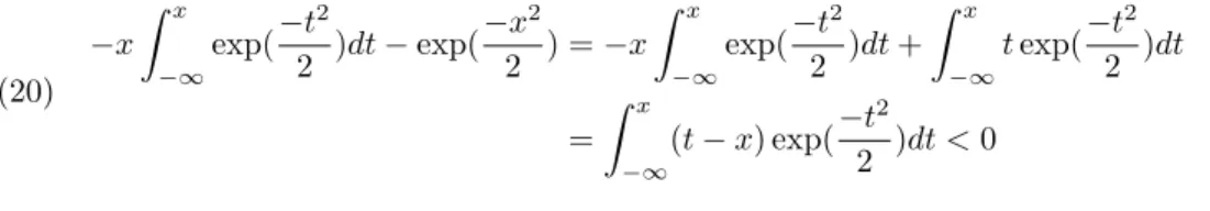
This is a convex function, a fact which is well-known in related contexts, but which we state and prove in the supplementary materials for the sake of completeness. In view of the close relationship between this problem and the level-set formulation described next, for which there are no minimizers, we expect that minimization may not be entirely straightforward in the γ 1 limit. This is manifested in the presence of near-flat regions in the probit log likelihood function whenγ1.
Our variant on the probit methodology differs from that in [20] in several ways: (i) our prior Gaussian is scaled to have per-node variance one, whilst in [20] the per node variance is a hyper-parameter to be determined; (ii) our prior is supported on
U =q0⊥ whilst in [20] the prior precision is found by shifting Land taking a possibly fractional power of the resulting matrix, resulting in support on the whole of RN; (iii) we allow for a scale parameter γ in the observational noise, whilst in [20] the parameterγ= 1.
3.2. Level-Set. This method is designed for problems considerably more general than classification on a graph [24]. For the current application, this model is exactly the same as probit except for the order in which the noiseη(j) and the thresholding functionS(u) is applied in the definition of the data.
PriorWe again take as prior foru, the Gaussianµ0. Thus P(u)∝exp −1 2hu, P ui . LikelihoodFor anyj ∈Z0
y(j) =S u(j)+η(j) with theη(j) drawn i.i.d fromN(0, γ2).Then
P y(j)|u(j)∝exp− 1 2γ2|y(j)−S (u(j) |2. PosteriorBayes’ Theorem gives posteriorµls with pdf
Pls(u|y)∝exp −1 2hu, P ui −Φls(u;y) where Φls(u;y) = X j∈Z0 1 2γ2|y(j)−S u(j) |2.
We letνls denote the pushforward underS ofµls:νls=S]µls.
MAP Estimator FunctionalThe negative of the log posterior is, in this case, given by
Jls(u) =
1
2hu, P ui+ Φls(u;y).
However, unlike the probit model, the Bayesian level-set method has no MAP esti-mator – the infimum ofJlsis not attained and this may be seen by noting that, if the
infumum was attained at any non-zero pointu? thenu? would reduce the objective
function for any ∈(0,1); however the point u? = 0 does not attain the infimum.
This proof is detailed in [24] for a closely related PDE based model, and the proof is easily adapted.
3.3. Atomic Noise Model. This is a variant on the level-set method, but deals with the fact that categorical data, whilst maybe noisy, will often be discrete. The resulting data model could also be used within the Ginzburg-Landau formulation in the next subsection, but we do not describe this explicitly. The prior we employ is the Gaussianµ0, and in contrast to the level-set method, but like the probit method, the observation is assumed to take values in the set{±1}. In the atomic noise model the reporting of those values is accompanied by specified error rates [34], determined
by the parameters p, q. Taking p=q= 1 in the following corresponds to exact data with no error and is the same as level-set thresholding, or probit, in the limitγ→0. PriorWe again take as prior foruthe Gaussianµ0.Thus
P(u)∝exp −1 2hu, P ui .
LikelihoodWe assume that the observation has the sign ofuwith a specified prob-ability. To be precise we assume that we have,
P(y= +1|u) =p, u≥0, P(y= +1|u) = 1−q, u <0 and
P(y=−1|u) = 1−p, u≥0, P(y=−1|u) =q, u <0.
This defines a piecewise constant function ofu, with discontinuity atu= 0, for each valuey∈ {±1}: we call this functionχ(u;y).In particular we have
P(y(j)|u(j)) =χ(u(j);y(j))
PosteriorBayes’ Theorem gives posteriorµatwith pdf
Pat(u|y)∝exp −1 2hu, P ui −Φat(u;y) . where Φat(u;y) =− X j∈Z0 logχ(u(j);y(j)).
We letνatdenote the pushforward underS ofµat:νat=S]µat.
MAP Estimator FunctionalThis is the minimizer of the negative of the log pos-terior. Thus we minimize the objective function:
Jat(u) =
1
2hu, P ui+ Φat(u;y).
We will not consider numerical methods for the atomic noise model because of space limitations. However it may be a natural choice for some measurement scenarios, hence its inclusion in this paper. Its behaviour is very similar to the Bayesian level set method because its likelihood is also piecewise constant with respect to latent variable u; and as with the Bayesian level set there is no minimizer for the MAP estimation problem.
3.4. Ginzburg-Landau. For this model, we take as prior the Ginzburg-Landau measureν0defined by (6), and employ a Gaussian likelihood for the observed labels. This construction gives the Bayesian posterior whose MAP estimator is the objective function introduced and studied in [5].
PriorWe define prior onv to be the Ginzburg-Landau measureν0given by (6) with density
P(v)∝e−GL(v).
LikelihoodFor anyj ∈Z0
y(j) =v(j) +η(j) with theη(j) drawn i.i.d fromN(0, γ2).Then
P y(j)|v(j)∝exp− 1 2γ2|y(j)−v(j)| 2. 11
PosteriorRecalling that P =c−1Lwe see that Bayes’ Theorem gives posterior νgl with pdf Pgl(v|y) ∝ exp −1 2hv, P vi −Φgl(v;y) , Φgl(v;y) := X j∈Z W v(j)+X j∈Z0 1 2γ2|y(j)−v(j)| 2.
MAP Estimator This is the minimizer of the negative of the log posterior. Thus we minimize the following objective function overU:
Jgl(v) =
1
2hv, P vi+ Φgl(v;y).
This objective function was introduced in [5] as a relaxation of the min-cut problem, penalized by data; the relationship to min-cut was studied rigorously in [40]. The minimization problem for Jgl is non-convex and has multiple minimizers, reflecting
the combinatorial character of the min-cut problem of which it is a relaxation.
3.5. Small Label Noise Limit. In the small label noise limitγ= 0 the probit and level-set posteriors coincide with the atomic noise model in the limit where p=
q= 1. Furthermore all models then take the form of the Gaussian priorµ0conditioned
to be positive on labelled nodes wherey(j) = 1 and to be negative on labelled nodes where y(j) = −1. This can be linked with the original work of Zhu et al [49, 50] which based classification on the measureµ0 conditioned to take the value exactly 1
on labelled nodes where y(j) = 1 and conditioned to take the value exactly −1 on labelled nodes where y(j) = −1.Thus we see explicit connections between a variety of different Bayesian formulations of graph-based semi-supervised learning.
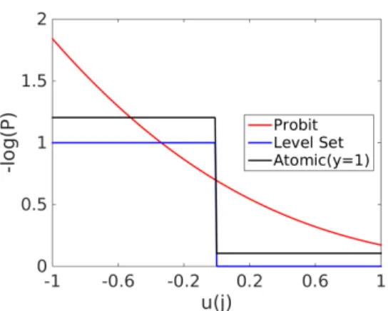
3.6. Uncertainty Quantification for Graph Based Learning. In Figure1 we plot the component of the negative log likelihood at a labelled nodej, as a function of the latent variableu=u(j) with datay=y(j) fixed, for the probit, Bayesian level-set, and atomic noise models. The log likelihood for the Ginzburg-Landau formulation is not directly comparable as it is a function of the relaxed label variablev(j), with respect to which it is quadratic with minimum at the data pointy(j).
The probit, Bayesian level-set, and atomic noise models lead to posterior distribu-tionsµ(with different subscripts) in latent variable space, and pushforwardsν (also with different subscripts) in label space. The Ginzburg-Landau formulation leads to a measure νgl in label space. Uncertainty quantification in the widest sense is con-cerned with completely characterizing these posterior distributions. In practice this may be acheived by sampling using MCMC methods. In this paper we will study four measures of uncertainty:
• we will study the empirical pdfs of the latent and label variables at certain nodes;
• we will study the posterior mean of the label variables at certain nodes; • we will study the posterior variance of the label variables averaged over all
nodes;
• we will use the posterior mean or variance to order nodes into those whose classificaions are most uncertain and those which are most certain.
For the probit, level-set and atomic models, we interpret the thresholded variable
l=S(u) as the binary label assignments corresponding to a real-valued configuration
u. The node-wise posterior mean ofl can be used as a useful confidence score of the 12
Fig. 1.Plot of a component of the negative log likelihood for a fixed nodej. We setγ= 1/√2 for probit and Bayesian level-set, andp= 0.8,q= 0.7for atomic noise model. SinceΦ(u(j); 1) = Φ(−u(j);−1)for probit and Bayesian level-set, we omit the plot fory(j) =−1.
class assignment of each node. The node-wise posterior meansl
j is defined as
(8) slj:=Eν(l(j)),
with respect to any of the posterior measures (pushed forward from latent vari-able space for probit, level-set and atomic models) ν. Note that sl
j ∈ [−1,1] and
if q = ν(l(j) = 1) then q = 12(1 +sl
j). For binary labels l(j) ∈ {±1} the mean
also contains the variance information, and hence the formula (8) captures posterior variance. Specifically we have that
Varν(l(j)) = 4q(1−q) = 1−(slj) 2.
Later we will find it useful to consider the variance averaged over all nodes and hence define3 (9) Var(l) = 1 N N X j=1 Varν(l(j)).
Note that the maximum value obtained by Var(l) is 1. This maximum value is at-tained under all the prior distributions we use in this paper. The deviation from this maximum, under the posterior, is a measure of the information content of the labelled data. Note, however, that the prior does contain information about classifications, in the form of correlations between vertices; this is not captured in (9).
4. Algorithms. From Section 3, we see that for all of the models considered, the posteriorP(w|y) has the form
P(w|y)∝exp −J(w), J(w) = 1
2hw, P wi+ Φ(w))
for some function Φ, different for each of the four models (acknowledging that in the Ginzburg-Landau case the independent variable is w = v, real-valued relaxation of
3Strictly speaking Var(l) =N−1Tr Cov(l)
.
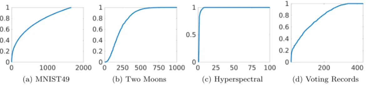
label space, where as for the other modelsw=uan underlying latent variable which may be thresholded by S(·) into label space.) Furthermore, the MAP estimator is the minimizer ofJ.Note that Φ is differentiable for the Ginzburg-Landau and probit models, but not for the level-set and atomic noise models. We introduce algorithms for both sampling (MCMC) and MAP estimation (optimization) that apply in this general framework. The sampler we employ does not use information about the gradient of Φ; the MAP estimation algorithm does, but is only employed on the Ginzburg-Landau and probit models. The samplers do use properties of the precision matrix P, which is proportional to the graph Laplcian L; in particular its spectral properties are relevant. Figure 2 demonstrates the spectral properties ofL for the four examples that we will apply our algorithms to in section5.
4.1. MCMC. We sample the posterior probability distribution using MCMC. To date probit models have typically been sampled by means of a Gibbs methodology. However for three reasons we consider sampling algorithms which apply directly on all the nodes Z. These are: (i) we wish to highlight methods which apply to the Ginzburg-Landau, level-set and atomic noise models which precludes the explicit conditionally Gaussian, or truncated Gaussian, form of the methods described for probit; (ii) all of our posterior distributions have a density with respect to the Gaussian
µ0– that is their densities are proportional to that ofµ0– and as a result we may use
MCMC methods which, in the case where the graph Laplacian has a limit [39], have the potential for delivering samples from the posterior in a number of steps which is independent of the dimensionN of the state space, as overviewed in [15]; (iii) these MCMC methods are well-adapted to the use of approximation methods which exploit structure in the spectral properties of the graph Laplacian. Other classes of MCMC methods, such as the Gibbs samplers in [1,22]; could be considered; and other priors, relaxing the Gaussian structure, could be considered; but in taking these directions then the development of MCMC methods withN−independent mixing rates which can also exploit approximations of the spectral properties of the graph Laplacian is an open research direction.
In order to induce scalability with respect to size of Z we use the pCN method described in [15] and introduced in the context of diffusions by Beskos et. al. in [7] and by Neal in the context of machine learning [31]. The standard random walk Metropolis (RWM) algorithm suffers from the fact that the optimal proposal variance or stepsize scales inverse proportionally to the dimension of the state space [35], which is the graph size N in this case. The pCN method is designed so that the proposal variance required to obtain a given acceptance probability scales independently of the dimension of the state space (here the number of graph nodesN), hence in practice giving faster convergence of the MCMC when compared with RWM [6]. We restate the pCN method as Algorithm1, and then follow with various variants on it in Algorithms 2 and3. In all three algorithmsβ ∈[0,1] is the key parameter which determines the efficiency of the MCMC method: small β leads to high acceptance probability but small moves; largeβ leads to low acceptance probability and large moves. Somewhere between these extremes is an optimal choice of β which minimizes the asymptotic variance of the algorithm when applied to compute a given expectation.
The valueξ(k)is a sample from the prior µ0. If the eigenvalues and eigenvectors ofLare all known then the Karhunen-Loeve expansion (10) gives
(10) ξ(k)=c12 N−1 X j=1 λ−12 j qjzj, 14
Algorithm 1pCN Algorithm 1: Input: L. Φ(u). u(0)∈U.
2: Output: M Approximate samples from the posterior distribution 3: Define: α(u, w) = min{1,exp(Φ(u)−Φ(w)}.
4: while k < M do
5: w(k)=p
1−β2u(k)+βξ(k), where ξ(k)∼ N(0, C) via Eq.(10).
6: Calculate acceptance probability α(u(k), w(k)).
7: Accept w(k)as u(k+1)with probability α(u(k), w(k)), otherwiseu(k+1)=u(k).
8: end while
wherecis given by (5), thezj, j= 1. . . N−1 are i.i.d centred unit Gaussians and the equality is in law.
4.2. Spectral Projection. For graphs with a large number of nodes N, it is prohibitively costly to directly sample from the distributionµ0, since doing so involves knowledge of a complete eigen-decomposition ofL, in order to employ (10). A method that is frequently used in classification tasks is to restrict the support of u to the eigenspace spanned by the first`eigenvectors with the smallest non-zero eigenvalues of L (hence largest precision) and this idea may be used to approximate the pCN method; this leads to a low rank approximation. In particular we approximate samples fromµ0 by (11) ξ`(k)=c 1 2 ` `−1 X j=1 λ− 1 2 j qjzj,
wherec`is given by (5) truncated afterj=`−1, thezjare i.i.d centred unit Gaussians and the equality is in law. This is a sample from N(0, C`) where C` = c`QΣ`Q∗
and the diagonal entries of Σ` are set to zero for the entries after `. In practice, to
implement this algorithm, it is only necessary to compute the first `eigenvectors of the graph LaplacianL. This gives Algorithm2.
Algorithm 2pCN Algorithm With Spectral Projection 1: Input: L. Φ(u). u(0)∈U.
2: Output: M Approximate samples from the posterior distribution 3: Define: α(u, w) = min{1,exp(Φ(u)−Φ(w)}.
4: while k < M do 5: w(k)=p 1−β2u(k)+βξ(k) ` , where ξ (k) ` ∼ N(0, C`) via Eq.(11).
6: Calculate acceptance probability α(u(k), w(k)).
7: Accept w(k)as u(k+1)with probability α(u(k), w(k)), otherwiseu(k+1)=u(k).
8: end while
9: return uk
The accuracy of Algorithm2 as an approximation of Algorithm 1 depends to a large extent on the size of the eigenvalues ofLin the following sense:
(12) E|ξ(k)|2−E|ξ(k)` | 2=c N−1 X j=1 λ−j1−c` `−1 X j=1 λ−j1
where the expectation is with respect to the centred unit Gaussians{zj}.Note that the examples shown in Figure2gives an indiciation of the quality of this approximation;
the size and number of the smallest eigenvalues of L play a very important role in determining whether the difference in (12) is small.
4.3. Spectral Approximation. Spectral projection often leads to good clas-sification results, but may lead to reduced posterior variance and a posterior distri-bution that is overly smooth on the graph domain. We propose an improvement on the method that preserves the variability of the posterior distribution but still only involves calculating the first ` eigenvectors of L. This is based on the empirical ob-servation that in many applications the spectrum of L saturates and satisfies, for
j ≥ `, λj ≈ ¯λ for some ¯λ. Such behaviour may be observed in b), c) and d) of Figure 2; in particular note that in the hyperspectal case ` N. We assume such behaviour in deriving the low rank approximation used in this subsection. (See sup-plementary materials for a detailed discussion of the graph Laplacian spectrum.) We define Σ`,oby overwriting the diagonal entries from`toN−1 with ¯λ−1.We then set C`,o=c`,oQΣ`,oQ∗, and generate approximate samples fromµ0 by setting
(13) ξ`,o(k)=c12 `,o `−1 X j=1 λ−12 j qjzj+c 1 2 `,oλ¯ −1 2 N−1 X j=` qjzj,
where c`,o is given by (5) with λj replaced by ¯λforj ≥`, the {zj} are centred unit Gaussians, and the equality is in law. Importantly samples according to (13) can be computed very efficiently. In particular there is no need to computeqj forj≥`, and the quantityPNj=`−1qjzj can be computed by first taking a sample ¯z∼ N(0, IN), and then projecting ¯zontoU`:= span(q`, . . . , qN−1). Moreover, projection ontoU`can be
computed only using{q1, . . . , q`−1}, since the vectors span the orthogonal complement
ofU`. Concretely, we have N−1 X j=` qjzj= ¯z− `−1 X j=1 qjhqj,z¯i,
where ¯z∼ N(0, IN) and equality is in law. Hence the samplesξ (k)
`,o can be computed
by (14) ξ`,o(k)=c12 `,o `−1 X j=1 λ−12 j qjzj+c 1 2 `,oλ¯ −1 2 ¯ z− `−1 X j=1 qjhqj,z¯i .
The error induced by this approximation can be characterized through the formula
(15) E|ξ(k)|2− E|ξ(k)`,o| 2= (c−c `,o) N−1 X j=1 λ−j1+c`,o N−1 X j=` λ−j1−¯λ−1.
Under the stated empirical properties of the graph Laplacian, we expect this to be a better approximation of the prior variance than the approximation leading to (12). The vectorξ`,o(k)is a sample fromN(0, C`,o) and results in Algorithm3.
4.4. MAP Estimation: Optimization. Recall that the objective function for the MAP estimation has the form 12hu, P ui+ Φ(u), where u is supported on the space U. For Ginzburg-Landau and probit, the function Φ is smooth, and we can use a standard projected gradient method for the optimization. SinceL is typically
(a) MNIST49 (b) Two Moons (c) Hyperspectral (d) Voting Records
Fig. 2. Spectra of graph Laplacian of various datasets. See Sec.5for the description of the datsets and graph construction parameters.
Algorithm 3pCN Algorithm With Spectral Approximation 1: Input: L. Φ(u). u(0)∈U.
2: Output: M Approximate samples from the posterior distribution 3: Define: α(u, w) = min{1,exp(Φ(u)−Φ(w)}.
4: while k < M do
5: w(k)=p1−β2u(k)+βξ`,o(k), where ξ`,o(k)∼ N(0, C`,o) via Eq.(14).
6: Calculate acceptance probability α(u(k), w(k)).
7: Accept w(k)as u(k+1)with probability α(u(k), w(k)), otherwiseu(k+1)=u(k). 8: end while
9: return uk
ill-conditioned, it is preferable to use a semi-implicit discretization as suggested in [5], as convergence to a stationary point can be shown under a graph independent learning rate. Furthermore, the discretization can be performed in terms of the eigen-basis{q1, . . . , qN−1}, which allows us to easily apply spectral projection when only a
truncated set of eigenvectors is available. We state the algorithm in terms of the (pos-sibly truncated) eigenbasis below. HereP`is an approximation toP found by setting
P`=Q`D`Q∗` whereQ` is the matrix with columns{q1,· · ·, q`−1}andD`= diag(d)
ford(j) =c`λj, j= 1,· · ·, `−1.ThusPN−1=P.
Algorithm 4Linearly-Implicit Gradient Flow with Spectral Projection 1: Input: Qm= (q1, . . . qm), Λm= (λ1, . . . , λm), Φ(u),u(0)∈U.
2: while k < M do
3: u(?)=u(k)−β∇Φ(u(k)) 4: u(k+1)= (I+βPm)−1u(?)
5: end while
5. Numerical Experiments. In this section we conduct a series of numerical experiments on four different data sets that are representative of the field of graph semi-supervised learning. There are four main purposes for the experiments. First we perform uncertainty quantification, as explained in subsection 3.6. Secondly, we study the spectral approximation and projection variants on pCN sampling as these scale well to massive graphs. Finally we make some observations about the cost and practical implementation details of these methods, for the different Bayesian models we adopt; these will help guide the reader in making choices about which algorithm to use. We present the results for MAP estimations in the supplementary materials,
alongside the proof of convexity of the Probit MAP estimator.
The quality of the graph constructed from the feature vectors is central to the performance of any graph learning algorithms. In the experiments below, we follow the graph construction procedures used in the previous papers [5, 23,29]; those pa-pers, together, applied graph partitioning to all of the datasets that we use here and so provide important guidance. Moreover, we have verified that for all the reported experiments below, the graph parameters are in a range such that spectral clustering gives a reasonable performance. The methods we employ lead to refinements over spectral clustering (improved classification) and, of course, to uncertainty quantifica-tion (which spectral clustering does not address).
5.1. Data Sets. We introduce the data sets and describe the graph construction for each data set. In all cases we numerically construct the weight matrixA, and then the graph LaplacianL.4
5.1.1. Two Moons. The two moons artificial data set is constructed to give noisy data which lies near a nonlinear low dimensional manifold embedded in a high dimensional space [13]. The data set is constructed by sampling N data points uni-formly from two semi-circles centered at (0,0) and (1,0.5) with radius 1, embed-ding the data in Rd, and adding Gaussian noise with standard deviation σ. We set N = 2,000 andd= 100 in this paper; recall that then the graph size is N and each feature vector has lengthd. We will conduct a variety of experiments with different labelled data size J, and in particular study variation with J. The default value, when not varied, isJ at 3% ofN, with the labelled points chosen at random.
We take each data point as a node on the graph, and construct a fully connected graph using the self-tuning weights of Zelnik-Manor and Perona [46], with K = 10. Specifically we letxi,xj be the coordinates of the data points iandj. Then weight
wij from itoj is defined by
(16) wij= exp−kxi−xjk
2
2τiτj
,
whereτj is the distance of theK-th closest point to the nodej.
5.1.2. House Voting Records from 1984. This dataset contains the voting records of 435 U.S. House of Representatives; for details see [5] and the references therein. The votes were recorded in 1984 from the 98thUnited States Congress, 2nd
session. The votes for each individual is vectorized by mapping a yes vote to 1, a no vote to−1, and an abstention/no-show to 0. The data set contains 16 votes that are believed to be well-correlated with partisanship, and we use only these votes as feature vectors for constructing the graph. Thus the graph size is N = 435, and feature vectors have length d = 16. The goal is to predict the party affiliation of each individual. We pick 3 Democrats and 2 Republicans at random to use as the observed class labels; thus J = 5 corresponding to less than 1.2% of fidelity points. We construct a fully connected graph with weights given by (16) withτj =τ = 1.25 for all nodesj.
5.1.3. MNIST. The MNIST database consists of 70,000 images of size 28×28 pixels containing the handwritten digits 0 through 9; see [26] for details. Since in this paper we focus on binary classification, we only consider pairs of digits. To speed up
4The weight matrixAis symmetric in theory; in practice we find that symmetrizing via the map
A7→1 2A+ 1 2A ∗is helpful. 18
calculations, we subsample randomly 2,000 images from each digit to form a graph with N = 4,000 nodes; we use this for all our experiments except in subsection5.4 where we use the full data set of sizeN =O(104) for digit pair (4,9) to benchmark
computational cost. The nodes of the graph are the images and as feature vectors we project the images onto the leading 50 principal components given by PCA; thus the feature vectors at each node have lengthd= 50.We conduct a variety of experiments with different labelled data dimension J, and in particular study variation with J. The default value, when not varied, isJ at 4% ofN, with the labelled points chosen at random. We construct aK-nearest neighbor graph with K = 20 for each pair of digits considered. Namely, the weights Aij are non-zero if and only if one of i or j
is in theK nearest neighbors of the other. The non-zero weights are set using (16) withK= 20. This is the only example we consider in this paper that does not have a fully connected graph.
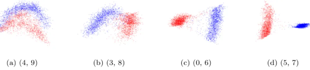
We choose the four pairs (5,7), (0,6), (3,8) and (4,9). These four pairs exhibit increasing levels of difficulty for classification. This fact is demonstrated in Figures 3a - 3d, where we visualize the datasets by projecting the dataset onto the second and third eigenvector of the graph Laplacian. Namely, each nodeiis mapped to the point (Q(2, i), Q(3, i))∈R2, where L=QΛQ∗.
(a) (4, 9) (b) (3, 8) (c) (0, 6) (d) (5, 7)
Fig. 3.Visualization of data by projection onto2ndand3rd eigenfuctions of the graph Lapla-cian for the MNIST data set, where the vertical dimension is the3rdeigenvector and the horizontal dimension the2nd. Each subfigure represents a different pair of digits. We construct a 20 nearest neighbour graph under the Zelnik-Manor and Perona scaling [46] as in(16)withK= 20.
5.1.4. HyperSpectral Image. The hyperspectral data set analysed for this project was provided by the Applied Physics Laboratory at Johns Hopkins University; see [12] for details. It consists of a series of video sequences recording the release of chemical plumes taken at the Dugway Proving Ground. Each layer in the spectral dimension depicts a particular frequency starting at 7,830 nm and ending with 11,700 nm, with a channel spacing of 30 nm, giving 129 channels; thus the feature vector has lengthd = 129. The spatial dimension of each frame is 128×320 pixels. We select 7 frames from the video sequence as the input data, and consider each spatial pixel as a node on the graph. Thus the graph size isN = 128×320×7 = 286,720. The classification problem is to classify pixels that represent the chemical plumes against pixels that are the background.
We construct a fully connected graph with weights given by the cosine distance:
wij =
hxi, xji kxikkxjk
.
This distance is small for vectors that point in the same direction, and is insensitive to their magnitude. We consider the symmetric Laplacian defined in (1). Because
it is computationally prohibitive to compute eigenvectors of a Laplacian of this size, we apply the Nystr¨om extension [44, 17] to obtain an approximation to the true eigenvectors and eigenvalues; see [5] for details pertinent to the set-up here. We emphasize that each pixel in the 7 frames is a node on the graph and that, in particular, pixels across the 7 time-frames are also connected. Since we have no ground truth labels for this dataset, we generate known labels by setting the segmentation results from spectral clustering as ground truth. The default value of J is 8,000, and labels are chosen at random. This corresponds to labelling around 2.8% of the points. We only plot results for the last 6 frames of the video sequence since the first frame does not contain the chemical plume.
5.2. Uncertainty Quantification. In this subsection we demonstrate both the feasibility, and value, of uncertainty quantification in graph classification methods. We employ the probit and the Bayesian level-set model for most of the experiments in this subsection; we also employ the Ginzburg-Landau model but since this can be slow to converge, due to the presence of local minima, it is only demonstrated on the voting records dataset. The atomic noise model has a similar piecewise constant log likelihood as for the Bayesian level-set method, and so we omit experiments on the atomic noise model. The pCN method is used for sampling on various datasets to demonstrate properties and interpretations of the posterior.
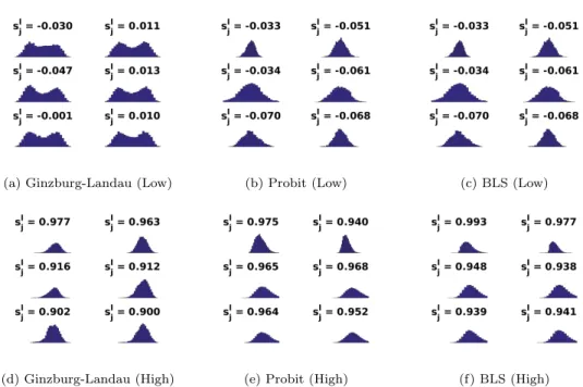
5.2.1. Visualization of Marginal Posterior Density. In this subsection, we contrast the posterior distributionP(v|y) of the Ginzburg-Landau model with that of the probit and Bayesian level-set (BLS) models. The graph is constructed from the voting records data with the fidelity points chosen as described in subsection 5.1. In Figure 4 we plot the histograms of the empirical marginal posterior distribution on P(v(i)|y) andP(u(i)|y) for a selection of nodes on the graph. For the top row of Figure 4, we select 6 nodes with “low confidence” predictions, and plot the empirical marginal distribution ofufor probit and BLS, and that of v for the Ginzburg-Landau model. Note that the same set of nodes is chosen for different models. The plots in this row demonstrate the multi-modal nature of the Ginzburg-Landau distribution in contrast to the uni-modal nature of the probit posterior; this uni-modality is a consequence of Proposition1. For the bottom row, we plot the same empirical distributions for 6 nodes with “high confidence” predictions. In contrast with the top row, the Ginzburg-Landau marginal for high confidence nodes is essentially uni-modal since most samples ofv evaluated on these nodes have a fixed sign.
We also observe that the pCN algorithm converges far more quickly for probit than for Ginzburg-Landau, because of the presence of multiple modes in the latter; this is manifest in the fact that the posteriors for Ginzburg-Landau are less well converged than for probit, for a similar amount of algorithmic time; this issue is quantified in subsection 5.4. This undesirable feature of Ginzburg-Landau sampling can be ameliorated by choosing a larger value of ; however this then leads to a probability measure which is further from the label space which it relaxes. The Bayesian level-set method behaves similarly to probit as is to be expected from the fact that, in the limitγ→0, they are formally identical as discussed in subsection3.5.
5.2.2. Posterior Mean as Confidence Scores. We construct the graph from the MNIST (4,9) dataset following subsection5.1. The noise varianceγis set to 0.1, and 4% of fidelity points are chosen randomly from each class. The probit posterior is used to compute (8). In Figure5 we demonstrate that nodes with scoresslj closer to the binary ground truth labels±1 look visually more uniform than nodes withsl
j
(a) Ginzburg-Landau (Low) (b) Probit (Low) (c) BLS (Low)
(d) Ginzburg-Landau (High) (e) Probit (High) (f) BLS (High)
Fig. 4. Visualization of marginal posterior density for low and high confidence predictions across different models. Each image plots the empirical marginal posterior density of a certain node
i, obtained from the histogram of 1×10⁵ approximate samples using pCN. Columns in the figure
(e.g. a) and d)) are grouped by model. From left to right, the models are Ginzburg-Landau, probit, and Bayesian level-set respectively. From the top down, the rows in the figure (e.g. a)-c)) denote the low confidence and high confidence predictions respectively. For the top row, we select6nodes with the lowest absolute value of the posterior meansl
j, defined in Eq.(8), averaged across three models. Note that the same set of nodes is chosen for different models. These nodes represent outliers in the dataset that are hard to classify, and hence more likely to induce a multi-modal marginal in the Ginzburg-Landau model. For the bottom row, we select nodes with the highest average posterior meanslj. These nodes represent nodes that are classified with greatest certainty to the class label +1. We present the posterior mean sl
j on top of the histograms for reference. The experiment parameters are: = 10.0,γ= 0.6,β= 0.1for the Ginburg-Landau model, andγ= 0.5,β= 0.2for the probit and BLS model.
far from those labels. This shows that the posterior mean contains useful information which differentiates between outliers and inliers that align with human perception.
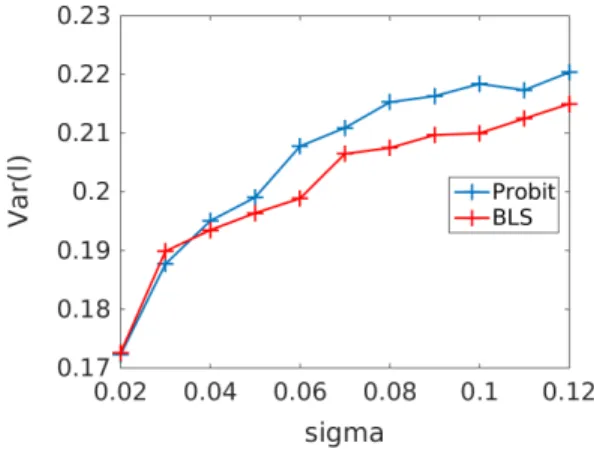
5.2.3. Posterior Variance as Uncertainty Measure. In this set of experi-ments, we show that the posterior distribution of the label variablel=S(u) captures the uncertainty of the classification problem. We use the posterior variance ofl, aver-aged over all nodes, as a measure of the model variance; specifically formula (9). We study the behaviour of this quantity as we vary the level of uncertainty within cer-tain inputs to the problem. We demonstrate empirically that the posterior variance is approximately monotonic with respect to variations in the levels of uncertainty in the input data, as it should be; and thus that the posterior variance contains useful information about the classification. We select quantities that reflect the separability of the classes in the feature space.
Figure6plots the posterior variance Var(l) against the standard deviationσof the noise appearing in the feature vectors for the two moons dataset; thus points generated on the two semi-circles overlap more asσincreases. We employ a sequence of posterior
(a) Fours in MNIST (b) Nines in MNIST
Fig. 5. “Hard to classify” vs “easy to classify” nodes in the MNIST (4,9)dataset under the
probit model. Here the digit “4” is labeled +1 and “9” is labeled -1. The top (bottom) row of the left column corresponds to images that have the lowest (highest) values ofsl
jdefined in (8)among images that have ground truth labels “4”. The right column is organized in the same way for images with ground truth labels9except the top row now corresponds to the highest values ofsl
j. Higherslj indicates higher confidence that imagejis a4and not a “9”, hence the top row could be interpreted as images that are “hard to classify” by the current model, and vice versa for the bottom row. The graph is constructed as in Section5, andγ= 0.1,β= 0.3.
computations, using probit and Bayesian level-set, for σ= 0.02 : 0.01 : 0.12. Recall that N = 2,000 and we choose 3% of the nodes to have the ground truth labels as observed data. Within both models, γ is fixed at 0.1. A total of 1×10⁴ samples
are taken, and the proposal varianceβ is set to 0.3. We see that the mean posterior variance increases with σ, as is intuitively reasonable. Furthermore, because γ is small, probit and Bayesian level-set are very similar models and this is reflected in the similar quantitative values for uncertainty.
Fig. 6.Mean Posterior Variance defined in (9)versus feature noiseσfor the probit model and the BLS model applied to the Two Moons Dataset with N = 2,000. For each trial, a realization of the two moons dataset under the given parameterσis generated, and3%of nodes are randomly chosen as fidelity. We run20trials for each value ofσ, and average the mean posterior variance across the20trials in the figure. We setγ= 0.1andβ= 0.3for both models.
A similar experiment studies the posterior label variance Var(l) as a function of the pair of digits classified within the MNIST data set. We choose 4% of the nodes as labelled data, and set γ= 0.1. The number of samples employed is 1×10⁴ and the
proposal varianceβis set to be 0.3. Table1shows the posterior label variance. Recall that Figures 3a - 3d suggest that the pairs (4,9),(3,8),(0,6),(5,7) are increasingly easy to separate, and this is reflected in the decrease of the posterior label variance shown in Table1.
Digits (4, 9) (3, 8) (0, 6) (5, 7) probit 0.1485 0.1005 0.0429 0.0084
BLS 0.1280 0.1018 0.0489 0.0121
Table 1
Mean Posterior Variance of different digit pairs for the probit model and the BLS model applied to the MNIST Dataset. The pairs are organized from left to right according to the separability of the two classes as shown in Fig.3a-3d. For each trial, we randomly select4%of nodes as fidelity. We run10trials for each pairs of digits and average the mean posterior variance across trials. We setγ= 0.1andβ= 0.3for both models.
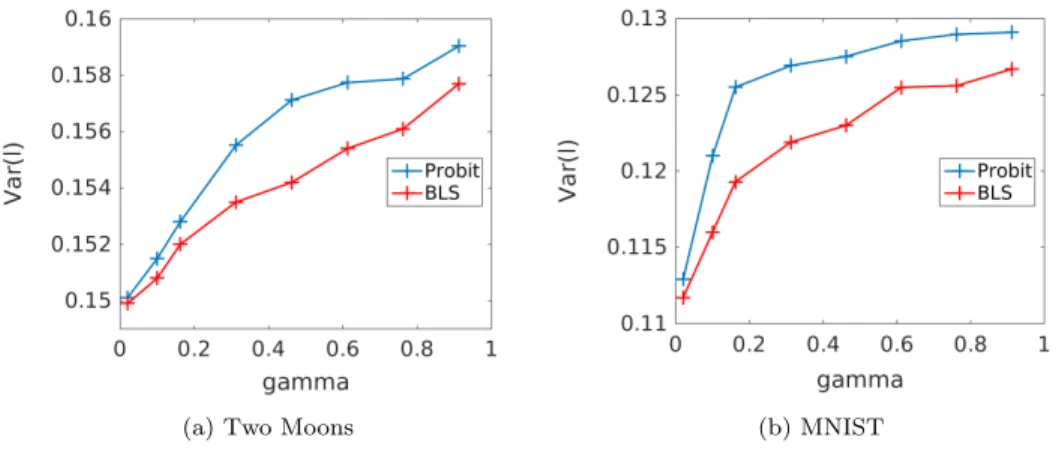
The previous two experiments in this subsection have studied posterior label variance Var(l) as a function of variation in the prior data; specifically as a function of the noise defining the feature vectors in two moons, and on the pair of digits used to classify in MNIST. We now turn and study how posterior variance changes as a function of varying the likelihood information, again for both two moons and MNIST data sets. In the two moons data set we freeze the feature vector noise atσ= 0.06. In Figures7aand7b, for the two moons and MNIST (4,9) data sets respectively, we plot the posterior label variance against the percentage of nodes observed. We observe that the observational variance decreases as the amount of labelled data increases. Figures 8a and 8bplot the posterior label variance as the observational noise γ is varied in the probit model, for both the two moons and MNIST (4,9) data sets; we fix 3% and 4% of randomly chosen nodes as observed labels in parts (a) and (b) of the figure respectively. Note that, as the observational variance increases, so too does the posterior label variance. Furthermore the level set and probit formulations produce similar answers forγ small, reflecting the discussion in subsection3.5.
In summary of this subsection, the label posterior variance Var(l) behaves in-tuitively as expected as a function of varying the prior and likelihood information that specify the statistical probit model and the Bayesian level-set model; further-more these two Bayesian models produce quantitatively similar reults because they are formally identical when noiseγ→0.The uncertainty quantification thus provides useful, and consistent, information that can be used to inform decisions made on the basis of classifications.
5.3. Spectral Approximation and Projection Methods. Here we discuss Algorithms2and 3, designed to approximate the full (but expensive on large graps) Algorithm1. In the first subsection we consider the voting records problem. This is small enough to compare the posterior distribution obtained from spectral projection and approximation with full sampling, and thereby verify their properties. Armed with this information we then study the hyperspectral problem in the next subsection; this problem is too large to be amenable to full sampling.
5.3.1. Applications to Voting Records. We study how the spectral projec-tion and approximaprojec-tion methods, Algorithm 2 and Algorithm 3, compare in perfor-mance with the full posterior distribution sampled via Algorithm 1. We do this by comparing the posterior mean of the thresholded variable sl
j in each case, and the
results are shown in Figure9. This clearly demonstrates that spectral projection does 23
(a) Two Moons (b) MNIST49
Fig. 7. Mean Posterior Variance as in (9)versus percentage of labelled points for the probit model and the BLS model applied to the Two Moons dataset and the 4-9 MNIST dataset. For two moons, we fixN= 2,000andσ= 0.06. For each trial, we generate a realization of the two moons dataset while the MNIST dataset is fixed, and select at random a certain percentage of nodes as labelled. We run20trials for each percentage of fidelity, and average the mean posterior variance across trials. We setγ= 0.1andβ= 0.1for both models.
(a) Two Moons (b) MNIST
Fig. 8. Mean Posterior Variance as in (9)versus the noise parameterγ, applied to the Two Moons dataset and the 4-9 MNIST dataset. For two moons, we fixN= 2,000and σ= 0.06. For each trial, we generate a realization of the two moons dataset while the MNIST dataset if fixed, and select randomly4%percentage of nodes as labelled. We run20trials for each percentage of fidelity, and average the mean posterior variance across trials. We setγas in the figure axis andβ= 0.3 for both models.
not perform as well as spectral approximation: Algorithm3yields results close to the full posterior obtained from Algorithm 1. In contrast the spectral projection Algo-rithm2 tends to underestimate the posterior variance, resulting in mean label values biased towards the values−1 or 1.
5.3.2. Applications to Hyperspectral Imaging. In Figures 10 and 11 we apply the Bayesian level-set model to the hyperspectral image dataset; the results for probit are similar (when we use smallγ) but have greater cost per step, because of the cdf evaluations required for probit. The figures show that the posterior mean
Fig. 9. Node-wise posterior mean slj of the full Laplacian, spectral truncation, and spectral approximation method of the probit model with the voting records dataset. The horizontal axis denotes the index of the nodes (voters), and the vertical axis denotes the values ofsl
j of the nodej. The per node mean absolute difference for spectral projection versus full is0.1577; it is0.0261 for spectral approximation versus full. We setγ= 0.1andβ= 0.3, and set the truncation level`= 150.
sl
j is able to differentiate between different concentrations of the plume gas. We
have also coloured pixels with|sl
j|<0.4 in red to highlight the regions with greater
levels of uncertainty. We observe that the red pixels mainly lie in the edges of the gas plume, which conforms with human intuition. As in the voting records example in the previous subsection, the spectral approximation method has greater posterior uncertainty, demonstrated by the greater number of red pixels in Fig.10 compared to Fig.11. We conjecture that the spectral approximation is closer to what would be obtained by sampling the full distribution, but we have not verified this as the full problem is too large to readily sample.
In Figure 12 we study optimization via the MAP estimator of the Ginzburg-Landau model, employing the Algorithm 4. Assuming that the results of Bayesian level-set sampling are accurate classifiers we deduce that the Ginzburg-Landau MAP estimator, since similar, is also a good classifier. However it would be unfeasible as the basis for sampling on this problem, again because of multi-modality of the posterior.
5.4. Comparitive Remarks About The Different Models. At a high level we have shown the following concerning the three models based on probit, level-set and Ginzburg-Landau:
• Probit and Bayesian level-set behave similarly, for posterior sampling, espe-cially for small γ, since they formally coincide when γ = 0. Bayesian level set is considerably cheaper to implement in Matlab because the norm cdf evaluations required for probit are expensive; this property of probit could perhaps be addressed directly via dedicated programming.
• Probit and Bayesian level-set are superior to Ginzburg-Landau for posterior sampling; this is because probit has log-concave posterior, whilst Ginzburg-Landau is multi-modal.
• Ginzburg-Landau provides the best hard classifiers, when used as an opti-25