1
Combining Electronic and Structural Features in Machine Learning Models to
Predict Organic Solar Cells Properties
Daniele Padula,* Jack D. Simpson, Alessandro Troisi*
Department of Chemistry, University of Liverpool, Liverpool L69 7ZD, U.K. E-mail: DP [email protected], AT [email protected]
Abstract
We present a translation of the chemical intuition in materials discovery, in terms of chemical similarity of efficient materials, into a rigorous framework exploiting Machine Learning. We computed equilibrium geometries and electronic properties (DFT) for a database of 249 Organic donor-acceptor pairs. We obtain similarity metrics between pairs of donors in terms of electronic and structural parameters, and we use such metrics to predict photovoltaic efficiency through linear and non-linear machine learning models. We observe that using only electronic or structural parameters leads to similar results, while considering both parameters at the same time improves the predictive capability of the models up to correlations of r≈0.7. Such correlation allows for reliable predictions of efficient materials, and lends to be coupled with combinatorial of evolutionary approaches for a more reliable virtual screening of candidate materials.
2
The design of new organic semiconductors for bulk heterojunction solar cells1-4 has attracted
many research initiatives5-7 highlighting the relevance and interest of any method enabling
the prediction of power conversion efficiency (PCE) of a solar cell from the knowledge of its constituents.8-12 From the theoretical point of view, the landscape is very complicated due to
the many physical processes occurring within a Photovoltaic Cell upon light absorption, such as exciton formation13 and migration,14 charge transport15 and recombination.16, 17 For this
reason, a microscopic modelling of each heterojunction is not a viable route for discovering new materials and materials prediction and can be limited to a few benchmark systems. Prediction for new semiconductors can become efficient through models depending on a limited number of easily computable parameters. One of the best known models of this type is Scharber’s model,18 which relies on a few reasonable assumptions and exploits only a few
electronic parameters of a donor-acceptor pair to obtain a prediction of photovoltaic efficiency. However, it is difficult to extend the model to include additional electronic parameters,8, 12, 19, 20 other descriptors of various nature (structural,9, 21 topological,22, 23
thermodynamic24-26), or other phenomena27 without formulating a completely new theory.
Adopting Machine Learning (ML) frameworks bypasses the step of theoretical development, creating a “black box” connection to properties otherwise inaccessible, at the cost of physical insight. Many different parameters of various nature can be included in the models, no hypotheses on the way the parameters are related among them or with the target property have to be made, unexpected correlations can be highlighted.20 In other words, given a set of
examples and input parameters, these algorithms fit an unknown function that mixes the parameters and returns an estimate of the target data. The great flexibility and variety of ML algorithms are beginning to be applied to materials discovery problems,6, 8, 10, 28-33 although
no consolidated methodology is emerging yet.9 Other groups reported ML approaches to
refine computed photovoltaic parameters, assuming the validity of Scharber’s model,29 or
bypassing any existing theory and including a wide range of electronic parameters, ignoring topological ones,8 or using complex structural representations34 to feed neural networks to
predict orbital energies.35 In recent work published by some of us8 a large number of
descriptors related to different physical phenomena was included. Each additional descriptor increases the computational cost related to obtaining the input, with the additional downside of missing elements connected to the chemistry of the material, in terms of structure, morphology, topology etc. Here we include a description of the chemical structure, which is less easy to correlate to the physical origin of the PCE, but implicitly includes the effects of chemical properties such as solubility, morphology etc. The definition of similarity in terms of both chemical and/or electronic parameters allowed us to obtain a set of highly predictive models targeting the photovoltaic efficiency of a donor-acceptor pair. Additionally, the small set of electronic parameters required in this model makes input data much easier to obtain. The main disadvantage, instead, is that kernel based methods scale with the square of examples in the data set, thus the reported method is feasible for data sets up to a few thousands entries.31 The proposed approach mimics in a mathematically rigorous fashion the
empirical exploration of new donors based on small chemical modifications of efficient molecules, providing new molecules with similar energy levels. Our results are important for applicative purposes, meaning that they provide reasonable predictions that can be coupled with combinatorial10 or evolutionary36 approaches to discover new materials.
3
Dataset. We built a database of 249 Organic donor-acceptor pairs that have been characterised in the literature between 2013 and 2017 (see SI for details on the search), mostly BHJ cells with a few (8) bilayer cells. We have gathered the experimental photovoltaic parameters (𝑉𝑂𝐶, 𝐽𝑆𝐶, 𝐹𝐹, 𝜂), and we have computed equilibrium geometries and four electronic properties at DFT level (HOMO energy for the donor 𝐸𝐷𝐻𝑂𝑀𝑂, LUMO energy for the donor 𝐸𝐷𝐿𝑈𝑀𝑂, LUMO energy for the acceptor 𝐸𝐴𝐿𝑈𝑀𝑂, the total internal reorganisation energy λ in vacuo for the oxidation of the donor and the reduction of the acceptor). The data set
contains only photovoltaic pairs where the acceptor is a fullerene acceptor, namely C60,
PC61BM or PC71BM. The choice of the low variability of the acceptors was consistent with
similar studies in the literature,8, 10, 29 and reflects the experimental way of scanning for new
donors, when the acceptor is kept fixed (or viceversa). In other words, the available experimental data do not explore uniformly the space of donor-acceptor but only a cross section with either few donors or few acceptors. Additionally, we would require much more complicated models to take into account also various acceptors, which we will explore in forthcoming work. Despite the low variability of acceptors, including in the input the 𝐸𝐴𝐿𝑈𝑀𝑂
parameter allows to take into consideration the same donor more than once, effectively increasing the size of the data set and allowing the model to “learn” the importance of energy level alignment. To consider structural similarities between donors, we relied on fingerprinting procedures commonly adopted in drug discovery,37, 38 which associate a
structural fingerprint (i.e. a vector) to each compound. We performed the analysis using both the Daylight and the Morgan fingerprinting algorithms.38 More details on the level of
calculation, software and strategies used are described in the SI. The data set is freely available to download as SI.
Scharber’s model results. Before discussing several machine learning algorithms, we report the predictions obtained with Scharber’s model, which is the most commonly used model for screening potential candidates on the basis of a few physical assumptions (described in ref
18). According to this model, the open circuit voltage (𝑉
𝑂𝐶), short circuit current (𝐽𝑆𝐶), and
power conversion efficiency (PCE or 𝜂) can be computed from the frontier orbital energies of a donor/acceptor pair and the solar irradiance spectrum, according to Eq. 1.
𝑉𝑂𝐶𝑆𝑐ℎ = 1 𝑒(𝐸𝐷 𝐻𝑂𝑀𝑂− 𝐸 𝐴𝐿𝑈𝑀𝑂 ) − 0.3 V (1) 𝐽𝑆𝐶𝑆𝑐ℎ = 0.65 ⋅ ∫ 𝜙𝑝ℎ(𝜆) d𝜆 𝐸𝐷𝑔𝑎𝑝 0 𝜂𝑆𝑐ℎ =𝑉𝑂𝐶 𝑆𝑐ℎ⋅ 𝐽 𝑆𝐶𝑆𝑐ℎ⋅ 0.65 𝑃𝑖𝑛
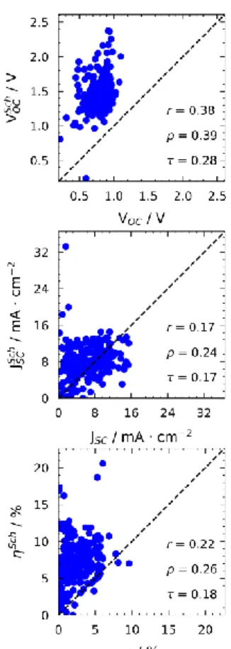
Numerical values in Eq. 1 are the result of empirical adjustment, e.g. the value appearing in the last equation of the set is a constant Fill Factor. The correlation between experimental and calculated properties is expressed in terms of three correlation coefficients, namely Pearson’s r, Spearman’s ρ, and Kendall’s τ. Fig. 1 summarizes the comparison between experimental and calculated properties with the correlation coefficients.
4
Fig. 1: comparison between computed and experimental photovoltaic properties. All properties are predicted very poorly by this model. For Fig. 1, we used Scharber’s model taking as input orbitals computed on gas phase optimised structures. However, we checked the effect of solvation by including an implicit solvation model39 (PCM) with two solvents
(toluene, chloroform) in our geometry optimisations, obtaining excellent correlations between orbital energies from gas phase and solvent geometries (see Fig. S11 in the Supporting Information). It is worth noticing that the energies of frontier orbitals of the studied molecules span a very small energy window of about 1.5 eV. In the literature are often reported very good correlations between experimental and computed orbital energies.40-42
However, they span much bigger energy windows or include much less data points. Our observations are in line with what already reported by others on similar molecules,29 and
highlight the limitations of DFT in the accurate discrimination of properties of molecules with “comparable” electronic structure, even when adopting more detailed descriptions including environmental effects.
Distance/Similarity Metrics. Measures of similarity between compounds will be used as input for the ML algorithms to be described below. Similarity measures are broadly used in cheminformatics and drug discovery and can help to detect overfitting, to establish a baseline for predictive methods thanks to zero cost procedures such as similarity-based regressions, or to mimic experimental discovery procedures.43 In our case, the properties defining each
example 𝐱𝑖 are a set of electronic properties (𝐱𝑖𝑒𝑙) and a molecular fingerprint (𝐱𝑖 𝑓𝑝
) and the distance is measured differently along these two sets of dimensions.
5
The distance between two examples 𝐱𝑖 and 𝐱𝑗 in terms of electronic parameters (in this case
𝐸𝐷𝐻𝑂𝑀𝑂, 𝐸𝐷𝐿𝑈𝑀𝑂, 𝐸𝐴𝐿𝑈𝑀𝑂, λ) can be computed as a Euclidean distance between the portions of the vectors containing electronic properties, namely 𝐱𝑖𝑒𝑙 and 𝐱𝑗𝑒𝑙, as in
𝐷𝑒𝑙(𝐱𝑖, 𝐱𝑗) = ‖𝐱𝑖𝑒𝑙− 𝐱𝑗𝑒𝑙‖2 (2)
The distance in terms of structural similarity is calculated from the Tanimoto similarity index (𝑇) between the portions of the vectors containing molecular fingerprints,10, 29, 37 namely 𝐱
𝑖 𝑓𝑝
and 𝐱𝑗𝑓𝑝, as in
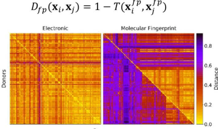
𝐷𝑓𝑝(𝐱𝑖, 𝐱𝑗) = 1 − 𝑇(𝐱𝑖𝑓𝑝, 𝐱𝑗𝑓𝑝) (3)
Fig. 2: distance matrices for the donors in the data set. Left: Euclidean distance between electronic parameters (see Eq. 2). Right: structural distance in terms of molecular fingerprints computed with two fingerprinting algorithms (see Eq. 1. Upper triangular:
Daylight fingerprints. Lower Triangular: Morgan fingerprints).
Molecular fingerprinting procedures to take into account structural similarities are commonly adopted in drug-discovery research,38 they are based on the nature of the atoms on the
molecules and on their chemical environment, and can be obtained by 2D representations of the molecules, i.e. the ability to draw them. This is very appealing because it opens up the possibility to obtain predictions without any computational data from more complicated approaches, allowing non experts to adopt very simple and quick models to predict properties of interest that are not accessible otherwise.
In Fig. 2 we report a graphical representation of the distances among pairs of donors in the data set. The distances in terms of electronic parameters show low variability across the data set. Concerning structural distance, Morgan fingerprints appear to perform better concerning selectivity, as there are less zones with a low value of the distance metric.
Prediction of Photovoltaic Parameters and Efficiency with k-NN Regression. A very simple prediction of a property is based only on similarity: if two molecules are similar, they will likely show similar behaviour. This algorithm reflects the way experimental trial and error research occurs: once a molecule with good properties is found, functionalisation allows the preparation of similar molecules in the hope they will have better properties.43 We computed
the predicted values of the properties as a weighted average of the experimental values for the k most similar molecules, with weights and proximity determined by the distances
6
expressed in Eqs. 2-3. The algorithm is known as k-NN (Nearest Neighbours) regression.44 The
predictions were computed using a Leave-One-Out (LOO) procedure, meaning that the training set used to compute distances is constituted by the whole data set except the point to be predicted. In other words, the experimental data relative to a certain point have not been used for its calculation, resulting in a truly predictive procedure. At the same time, the availability of experimental data makes the quality of models quantifiable through correlation metrics. The LOO cross-validation scheme was preferred over a k-fold scheme because it is expected to give better results due to the bigger size of training sets, and to give a lower variance of predictions because models will be trained on almost the same data.
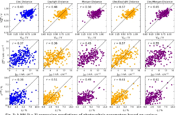
We used the distances reported in Eqs. 2-3 (with both Daylight and Morgan fingerprinting algorithms, where fingerprints are needed), and used various values of k. In Fig. 3 we report as an example the results for the predictions of photovoltaic cell parameters, for k=3 (results for other values of k are quantitatively similar as discussed in the SI). The algorithm can be used to predict directly 𝑉𝑂𝐶, 𝐽𝑆𝐶, 𝜂 and its results are illustrated in Fig. 3 using various definitions of distance.
Fig. 3: k-NN (k = 3) regression predictions of photovoltaic parameters based on various distances, indicated at the top of each column. Colours encode electronic properties only (blue), or the type of molecular fingerprint used (Daylight in yellow, Morgan in magenta).
RMSE data available in Table S1 (Supporting Information).
Considering a distance in terms of electronic parameters only (first column of Fig. 3) results in moderate correlation coefficients for the predictions, likely because the electronic properties are relatively homogeneous across the whole data set. Switching to a structural distance metric (second and third columns of Fig. 3), improves predictions sensibly, with little
7
dependence on the fingerprinting algorithm, as both Daylight and Morgan fingerprints give comparable results. In this case, we must stress the advantage that no quantum chemical calculations have to be run at all, as the distance metric results exclusively from a 2-D representation of molecules, i.e. the ability to draw them.
As a step forward we can consider a weighted average of the two distances
𝐷 = 𝛾1𝐷𝑒𝑙(𝐱𝑖, 𝐱𝑗) + 𝛾2𝐷𝑓𝑝(𝐱𝑖, 𝐱𝑗) (4) where the hyperparameters 𝛾1, 𝛾2 are chosen here to minimise the average RMSE of the
prediction with the LOO approach (see SI). The k-NN algorithm with a distance that includes both electronic and structural information (fourth and fifth columns of Fig. 3) results in substantially improved predictions with remarkable correlation between predicted and observed data (r > 0.6).
Prediction of Photovoltaic Efficiency with Kernel Ridge Regression. An algorithm such as k-NN is extremely rigid in considering only a fixed number of neighbours regardless of the density of data points and ignoring the non-linear relation between positions in the parameter space and property. A much more flexible algorithm, known as Kernel Ridge Regression (KRR),30, 31 will be considered next. This algorithm can be seen as a generalised
version of the least square procedure, where a non-linearity and regularisation have been introduced, and it is treated extensively in the SI and other literature contributions.30, 31 More
formally, we define a training set of N examples {(𝐱𝑖, 𝑦𝑖)}𝑖=1𝑁 , with 𝐱
𝑖 a vector containing the
inputs for the i-th example (e.g. electronic and or structural fingerprints), and the outputs 𝑦𝑖
(i.e. the target experimental property like 𝜂), are gathered in a vector 𝐲. Given an arbitrary scalar function 𝑓(𝐱𝑖, 𝐱𝑗), known as the kernel function,31 the predicted property 𝐲′ for a new
element with input property 𝐱′ is expressed by the KRR algorithm as
𝐲′ = 𝐲𝑇(𝐾 + 𝛼𝐼)−1𝜿′ (5)
where 𝐼 is the identity matrix, 𝛼 a regularisation hyperparameter, the matrix 𝐾 and vector 𝜿′
defined as 𝐾𝑖𝑗 = 𝑓(𝐱𝑖, 𝐱𝑗) and 𝜅𝑖′ = 𝑓(𝐱𝑖, 𝐱′). The kernel function 𝑓 is defined to represent
a measure of “distance” between any two coordinates in the parameters space. In this case we can use the distance between electronic properties and fingerprints to define a kernel as
𝑓(𝐱𝑖, 𝐱𝑗) = 𝑒−(𝛾1𝐷𝑒𝑙2(𝐱𝑖,𝐱𝑗)+𝛾2𝐷𝑓𝑝2 (𝐱𝑖,𝐱𝑗)) (6) This allows to introduce non-linearity, to use either electronic or structural information only, by setting 𝛾2 = 0 or 𝛾1 = 0 respectively, or to include both electronic and structural information in the model. Notice that if structural information are neglected by setting 𝛾2 = 0, Eq. 6 corresponds to adopting a Radial Basis Function kernel.31 The hyperparameters 𝛼, 𝛾
1
and/or 𝛾2 are determined via cross validation (see SI).
We obtained predictions of photovoltaic parameters to be used as input for Scharber’s model (see SI) and direct predictions of photovoltaic efficiencies using the kernels reported in Eq. 6 (with both Daylight and Morgan fingerprinting algorithms, where fingerprints are needed), using electronic input data standardised to zero average and unit standard deviation.
8
Predictions were obtained adopting a LOO scheme as described previously, taking advantage of the possibility that, for KRR, the LOO scheme can be implemented analytically45 and thus
results computationally cheaper in comparison to other cross-validation schemes.
Fig. 4: KRR predictions of photovoltaic efficiency based on various distance-based kernels, indicated at the top of each column. Colours encode electronic properties only (blue), or the
type of molecular fingerprint used (Daylight in yellow, Morgan in magenta). RMSE data available in Table S1 (Supporting Information).
The direct predictions of efficiency in Fig. 4 allow to obtain better predictions with respect to refining the input for Scharber’s model (see SI), and improve with respect to direct predictions adopting the simpler k-NN regression, as can be observed in the summary of correlation coefficients reported in Table 1. Adopting electronic distance only (first column of Fig. 4), we notice a significant improvement when using KRR, passing from r=0.38 to r=0.49. We tried to estimate the importance of each electronic feature for this model. Since for kernel-based methods feature importance cannot be defined, as the problem is formulated in the examples space, we decided to adopt a feature elimination procedure (see Table S3 in the Supporting Information), observing a little influence of the reorganisation energy λ, and a considerable importance for the 𝐸𝐷𝐿𝑈𝑀𝑂. Adopting structural distance only (second and third columns of Fig. 4), we obtain a significant improvement with Morgan fingerprints (r=0.49 to r=0.57) and a worse result with Daylight fingerprints (r=0.51 to r=0.43). Finally, when both distances are considered within KRR (fourth and fifth columns of Fig. 4), we again obtain a significant improvement with respect to using one distance only. Adopting a linear combination of distances with KRR, we also obtain better results with respect to the simpler k-NN algorithm, especially with Morgan fingerprints (r=0.61 to r=0.68).
For the best model, we obtain strong correlations (r ≈ 0.7, see Table 1, and Table S2 reporting additional correlation coefficients) that are comparable to the best reported so far in the literature,6, 8 improve significantly over naïve prediction strategies, and thus are good enough
to obtain reliable predictions of efficiencies, aimed at accelerating the discovery of new efficient materials. To assess the effect of specific structural features on our best model, we checked that the distribution of errors did not change significantly upon removal of entries containing a specific structural feature of interest through a Kruskal-Wallis test.46 As an
example, we report in the Supporting Information the distribution of errors obtained for our best model trained only on entries that do not contain Halogen atoms.
In conclusion, we have verified that Scharber’s model has very limited predictive properties when used in conjunction with DFT calculations. We have therefore explored a range of
9
machine learning algorithms combining electronic properties and topological information, obtaining highly predictive models. A simple k-NN model already yields correlations of ~0.6 between experiment and predictions, which can be improved up to ~0.7 by exploiting non-linear kernel methods. The introduction of structural similarity metrics mimics the approach adopted in experimental research, i.e. this approach can be seen as an implementation of “artificial chemical intuition”. Various improvements can be foreseen: analysis of larger data sets in terms of molecules and properties included, identification of figures of merit better than RMSE for the optimisation of hyperparameters, and coupling with combinatiorial or genetic searches to propose new high efficiency candidates.
Table 1: Values of Pearson’s correlation coefficient for the models used. The best model for predictions of 𝜂 is highlighted in bold.
Fig. Model Input Target
Property r 3 k-NN Elec 𝑉𝑂𝐶 0.43 3 k-NN Elec 𝐽𝑆𝐶 0.37 3 k-NN Elec 𝜂 0.38 3 k-NN Daylight 𝑉𝑂𝐶 0.48 3 k-NN Daylight 𝐽𝑆𝐶 0.36 3 k-NN Daylight 𝜂 0.51 3 k-NN Morgan 𝑉𝑂𝐶 0.50 3 k-NN Morgan 𝐽𝑆𝐶 0.45 3 k-NN Morgan 𝜂 0.49 3 k-NN Elec/Daylight 𝑉𝑂𝐶 0.57 3 k-NN Elec/Daylight 𝐽𝑆𝐶 0.57 3 k-NN Elec/Daylight 𝜂 0.61 3 k-NN Elec/Morgan 𝑉𝑂𝐶 0.65 3 k-NN Elec/Morgan 𝐽𝑆𝐶 0.55 3 k-NN Elec/Morgan 𝜂 0.61 4 KRR Elec 𝜂 0.49 4 KRR Daylight 𝜂 0.43 4 KRR Morgan 𝜂 0.57 4 KRR Elec/Daylight 𝜂 0.59 4 KRR Elec/Morgan 𝜼 0.68
Supporting Information
The Supporting Information includes an archive containing the coordinates of the optimised geometries of analysed molecules and a database of the properties gathered from quantum chemical calculations used as input for electronic distance calculations, details on the procedures adopted for data gathering and calculations, a detailed theoretical treatment of Kernel Ridge Regression, values of hyperparameters and metrics for the models used, additional figures and tables.
Acknowledgements
This work was supported by the ERC through Grant No. 615834. We are grateful to Dr. Stefano Caprasecca (Open University, Verizon Connect) for fruitful discussions.
10
References
1. G. J. Hedley, A. Ruseckas and I. D. Samuel, Chem. Rev., 2017, 117, 796-837.
2. S. Antohe, S. Iftimie, L. Hrostea, V. A. Antohe and M. Girtan, Thin Solid Films, 2017, 642, 219-231.
3. K. Wang, C. Liu, T. Meng, C. Yi and X. Gong, Chem. Soc. Rev., 2016, 45, 2937-2975.
4. L. Lu, T. Zheng, Q. Wu, A. M. Schneider, D. Zhao and L. Yu, Chem. Rev., 2015, 115, 12666-12731.
5. S. A. Lopez, E. O. Pyzer-Knapp, G. N. Simm, T. Lutzow, K. Li, L. R. Seress, J. Hachmann and A. Aspuru-Guzik, Sci. Data, 2016, 3, 160086.
6. E. O. Pyzer-Knapp, K. Li and A. Aspuru-Guzik, Adv. Funct. Mater., 2015, 25, 6495-6502. 7. J. Hachmann, R. Olivares-Amaya, A. Jinich, A. L. Appleton, M. A. Blood-Forsythe, L. R. Seress,
C. Román-Salgado, K. Trepte, S. Atahan-Evrenk, S. Er, S. Shrestha, R. Mondal, A. Sokolov, Z. Bao and A. Aspuru-Guzik, Energy Environ. Sci., 2014, 7, 698-704.
8. H. Sahu, W. Rao, A. Troisi and H. Ma, Advanced Energy Materials, 2018, DOI: 10.1002/aenm.201801032, 1801032.
9. D. C. Elton, Z. Boukouvalas, M. S. Butrico, M. D. Fuge and P. W. Chung, Sci. Rep., 2018, 8, 9059. 10. S. A. Lopez, B. Sanchez-Lengeling, J. de Goes Soares and A. Aspuru-Guzik, Joule, 2017, 1,
857-870.
11. Y. Liu, T. Zhao, W. Ju and S. Shi, J. Materiomics, 2017, 3, 159-177.
12. C. Schober, K. Reuter and H. Oberhofer, J Phys Chem Lett, 2016, 7, 3973-3977. 13. V. Janković and N. Vukmirović, Phys. Rev. B, 2015, 92.
14. O. V. Mikhnenko, P. W. M. Blom and T.-Q. Nguyen, Energy Environ. Sci., 2015, 8, 1867-1888. 15. V. Coropceanu, J. Cornil, D. A. da Silva Filho, Y. Olivier, R. Silbey and J. L. Bredas, Chem. Rev.,
2007, 107, 926-952.
16. C. M. Proctor, M. Kuik and T.-Q. Nguyen, Prog. Polym. Sci., 2013, 38, 1941-1960.
17. N. A. Ran, J. A. Love, M. C. Heiber, X. Jiao, M. P. Hughes, A. Karki, M. Wang, V. V. Brus, H. Wang, D. Neher, H. Ade, G. C. Bazan and T.-Q. Nguyen, Advanced Energy Materials, 2018, 8, 1701073. 18. M. C. Scharber, D. Mühlbacher, M. Koppe, P. Denk, C. Waldauf, A. J. Heeger and C. J. Brabec,
Adv. Mater., 2006, 18, 789-794.
19. R. P. Fornari, P. Rowe, D. Padula and A. Troisi, J Chem Theory Comput, 2017, 13, 3754-3763. 20. A. Kuzmich, D. Padula, H. Ma and A. Troisi, Energy Environ. Sci., 2017, 10, 395-401.
21. M. Rupp, A. Tkatchenko, K. R. Muller and O. A. von Lilienfeld, Phys. Rev. Lett., 2012, 108, 058301.
22. S. Bibi and J. Zhang, New J. Chem., 2016, 40, 3693-3704.
23. J. Mai, T.-K. Lau, J. Li, S.-H. Peng, C.-S. Hsu, U. S. Jeng, J. Zeng, N. Zhao, X. Xiao and X. Lu, Chem.
Mater., 2016, 28, 6186-6195.
24. S. Torabi, F. Jahani, I. Van Severen, C. Kanimozhi, S. Patil, R. W. A. Havenith, R. C. Chiechi, L. Lutsen, D. J. M. Vanderzande, T. J. Cleij, J. C. Hummelen and L. J. A. Koster, Adv. Funct. Mater., 2015, 25, 150-157.
25. J. Li, G. Zhang, D. M. Holm, I. E. Jacobs, B. Yin, P. Stroeve, M. Mascal and A. J. Moulé, Chem.
Mater., 2015, 27, 5765-5774.
26. F. Machui, S. Abbott, D. Waller, M. Koppe and C. J. Brabec, Macromol. Chem. Phys., 2011, 212, 2159-2165.
27. G. Sini, M. Schubert, C. Risko, S. Roland, O. P. Lee, Z. Chen, T. V. Richter, D. Dolfen, V. Coropceanu, S. Ludwigs, U. Scherf, A. Facchetti, J. M. J. Fréchet and D. Neher, Advanced Energy
Materials, 2018, 8, 1702232.
28. O. A. von Lilienfeld, Angew. Chem. Int. Ed. Engl., 2018, 57, 4164-4169.
29. E. O. Pyzer-Knapp, G. N. Simm and A. Aspuru Guzik, Mater. Horizons, 2016, 3, 226-233. 30. K. Vu, J. C. Snyder, L. Li, M. Rupp, B. F. Chen, T. Khelif, K.-R. Müller and K. Burke, Int. J. Quantum
Chem., 2015, 115, 1115-1128.
11
32. S. Nagasawa, E. Al-Naamani and A. Saeki, J Phys Chem Lett, 2018, 9, 2639-2646.
33. R. Visini, J. Arus-Pous, M. Awale and J. L. Reymond, J. Chem. Inf. Model., 2017, 57, 2707-2718. 34. K. T. Schutt, F. Arbabzadah, S. Chmiela, K. R. Muller and A. Tkatchenko, Nat. Comm., 2017, 8,
13890.
35. P. B. Jorgensen, M. Mesta, S. Shil, J. M. Garcia Lastra, K. W. Jacobsen, K. S. Thygesen and M. N. Schmidt, J. Chem. Phys., 2018, 148, 241735.
36. I. Y. Kanal, S. G. Owens, J. S. Bechtel and G. R. Hutchison, J. Phys. Chem. Lett., 2013, 4, 1613-1623.
37. D. Bajusz, A. Racz and K. Heberger, J Cheminform, 2015, 7, 20. 38. D. Rogers and M. Hahn, J. Chem. Inf. Model., 2010, 50, 742-754.
39. J. Tomasi, B. Mennucci and R. Cammi, Chem. Rev., 2005, 105, 2999-3093.
40. D. D. Méndez-Hernández, P. Tarakeshwar, D. Gust, T. A. Moore, A. L. Moore and V. Mujica, J.
Mol. Model., 2013, 19, 2845-2848.
41. C.-G. Zhan, J. A. Nichols and D. A. Dixon, J. Phys. Chem. A, 2003, 107, 4184-4195. 42. G. Zhang and C. B. Musgrave, J. Phys. Chem. A, 2007, 111, 1554-1561.
43. Q. Wang, J. J. van Franeker, B. J. Bruijnaers, M. M. Wienk and R. A. J. Janssen, J. Mater. Chem.
A, 2016, 4, 10532-10541.
44. N. S. Altman, Am. Stat., 1992, 46, 175-185.
45. Y. Zhao and K. Kwoh Chee, Proceedings of the 17th International Conference on Pattern
Recognition, 2004. ICPR 2004., 2004, 3, 494-497 Vol.493.