Knowledge-based design space exploration of wireless sensor networks

(1)

Knowledge-Based Design Space Exploration

of Wireless Sensor Networks

Paolo Roberto Grassi

1

, Ivan Beretta

2

, Vincenzo Rana

1,2

,

David Atienza

2

and Donatella Sciuto

1

1 _{Politecnico di Milano, DEI, Italy, {grassi, rana, sciuto}@elet.polimi.it}

2 _{École Polytechnique Fédérale de Lausanne, ESL, Switzerland, {ivan.beretta, david.atienza}@epfl.ch}

ABSTRACT

The complexity of Wireless Sensor Networks (WSNs) has been constantly increasing over the last decade, and the ne-cessity of efficient CAD tools has been growing accordingly. In fact, the size of the design space of a WSN has become large, and an exploration conducted by using semi-random algorithms (such as the popular genetic or simulated anneal-ing algorithms) requires an unacceptable amount of time to converge due to the high number of parameters involved. To address this issue, in this paper we introduce a knowledge-based design space exploration algorithm for the WSN do-main, which is based on a discrete-space Markov decision process (MDP). In order to enhance the performance of the proposed algorithm and to increase its scalability, we tai-lor the classical MDP approach to the specific aspects that characterize the WSN domain. We exploit domain-specific knowledge to choose the best node-level configuration in WSNs using slotted star topology in order to reduce the exploration time. The proposed approach has been tested on IEEE 802.15.4 star networks with various configurations of the number of nodes and their packet rates. Experi-mental results show that the proposed algorithm reduces the number of simulations required to converge, with re-spect to state-of-the-art algorithms (e.g., NSGA-II, PMA and MOSA), from 60 to 87%.

Categories and Subject Descriptors

C.4 [Computer Systems Organization]: Performance of Systems—Design studies, modeling techniques; C.3 [Computer Systems Organization]: Special-Purpose and Application-Based Systems—Real-time and embedded systems

General Terms

Design, Algorithms

Keywords

Design Space Exploration, Markov Decision Process, Wire-less Sensor Networks

Permission to make digital or hard copies of all or part of this work for personal or classroom use is granted without fee provided that copies are not made or distributed for profit or commercial advantage and that copies bear this notice and the full citation on the first page. To copy otherwise, to republish, to post on servers or to redistribute to lists, requires prior specific permission and/or a fee.

1. INTRODUCTION

The increasing complexity of Wireless Sensor Networks (WSNs) is leading towards the deployment of very sophis-ticated and ubiquitous networked systems. A WSN is com-posed by several nodes that communicate through a wire-less channel: these nodes are typically battery-powered, and equipped with low-performance processors and small mem-ories in order to reduce the power requirements. A common WSN node comprises five main components [19]: a pro-cessing element (microcontroller, processor, etc.), memory elements (RAM, SD, Flash, etc.), multiple communication layers (physical radio, MAC, Routing), a power supply and a sensing unit (including sensor, transducer, ADC). During the design phase, the contribution of all these components must be combined to identify the configuration that best fits the design objectives. The combination of different layers and the large number of configurable hardware and software parameters often generates an extremely large design space, which requires a powerful CAD algorithm to carry out the exploration.

A critical aspect of the Design Space Exploration (DSE) is the evaluation of a WSN configuration. Among the possible evaluation techniques, network models provide a deep un-derstanding of the network dynamics that can be exploited during the DSE, but their definition is generally difficult and requires a deep knowledge of the working domain [4]. As a consequence, evaluation is typically performed using exten-sive network simulations [7], which are more accurate and reusable. However, a WSN simulation may take from sev-eral minutes to hours (depending on the network size) to be completed, and it should be repeated tens of times (gener-ally more than 30) to mitigate the effects of randomness and ensure reliable statistical results.

In this paper, we propose a knowledge-based DSE al-gorithm that effectively tackles the design complexity of WSNs, by combining the domain knowledge of the analyti-cal models with the generality and the flexibility of network simulators. Unlike semi-random algorithms, which require an evaluation at each step, the proposed approach performs several moves by relying on a set of domain-specific rules, thus greatly reducing the number of simulations. For this purpose, we adapt theMarkov decision process (MDP) al-gorithm [5] to the WSN domain, and we solve its inherited scalability issues to face the large design spaces of WSNs. We also introduce a general domain knowledge for the most popular WSN MAC layer, i.e., the IEEE 802.15.4 [3], which can be reused on any WSN based on this protocol. Vali-dation results prove that the proposed approach effectively

(2)

reduces the number of simulations with respect to state-of-the-art semi-random algorithms from 60 to 87% on multiple real-world scenarios.

2. PROBLEM DEFINITION

In this section, we provide a characterization of the design space (denoted asS) of WSNs, in order to show the complex-ity of this kind of systems. The parameter space of a WSN is divided into two parts: a set ofnode parameters(Pn), which

can assume different values on each nodes, and a set of net-work parameters (Pr), which assume one value throughout

the whole network (or at least a part of it). For example, the memory size or the type of processor are specific of each node, hence they belong toPn, whereas the network

proto-col must be the same among the nodes, therefore it belongs toPr. Each parameterp∈(Pn∪Pr) is assigned to a discrete

set of values in an interval [pmin, pmax], whose cardinality is

denoted as|p|.

Node parameters heavily affect the design space size |S|, since each parameters can assume an independent value on each node. Thus, when network size (expressed in terms of the number of nodes, N) increases, then |S| increases exponentially. More formally, we can express the size of the design space of a WSN: |S|= Y p∈Pr |p| ! · Y q∈Pn |q| !N . (1)

To understand the order of magnitude of|S|, let us show a relatively small example for structural or environmental monitoring. Let us assume that 8 nodes are placed on a 2×2×2 tridimensional grid in the monitored area, and that the communication is regulated by the IEEE 802.15.4 MAC protocol [3]. Even without considering any hardware param-eter, the configuration of the MAC protocol itself contains a wide set of possible parameters inPr (e.g., theframeand

the beacon orders [3]) and inPn (e.g., the choice of using

the contention active communication, or the number of re-questedguaranteed time slots [3]). Overall, the design space contains approximately 290billions of solutions.

Thus, an extensive DSE would take an unacceptable amount of time when network simulation is the only viable way to evaluate a solution. As a consequence, a technique that is able to reduce the number of simulations is required.

3. STATE OF THE ART

Design space exploration is a well established research topic in many different fields, such as embedded architec-tures or system-level design. However, automatic DSE is still immature in WSN design, where the complexity of the network and the peculiarity of each application domain often push the developers towards manual andad hoc optimiza-tions (e.g., the work in [10] for wildlife monitoring).

The main obstacle towards the complete automation of the DSE of WSNs is a rapid and accurate evaluation of a solution. Currently, the two evaluation techniques [4] are models and simulations. Analytical models describe the WSN dynamics by means of a set of equations that pro-vide awhite-box view of the system, thus extensive analysis are possible. When a model-based evaluation is employed, the DSE is considerably faster compared to simulation-based

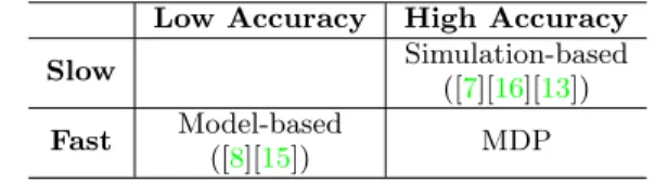
Table 1: Speed and accuracy of existing DSE tech-niques

Low Accuracy High Accuracy

Slow Simulation-based_([₇_][₁₆_][₁₃_])

Fast Model-based MDP

([8][15])

approaches, but the accuracy of the model is typically guar-anteed only for specific domains or for specific aspects of the WSN. In fact, only models that have been proposed for single classes of WSNs (e.g., [21] for body area networks) or for specific protocols (e.g. [11],[6] and [18] for three different operations of the IEEE 802.15.4 MAC layer) show an accu-racy that is comparable to a simulation. In [14] an MDP is used to detect optimal sensor node operation in order to meet the application requirements. In this case, the solution is identified analytically solving the MDP via custom reward functions. However, it requires an accurate model to both guide and evaluate the solutions, which is a very important limitation. On the other hand, simulations better profile all the aspects related to communication, energy and resource usage of distributed applications. However, a robust simu-lation takes several from minutes to hours, thus making it impractical for extensive DSEs.

In this context, the evaluation technique heavily affects the choice of the optimization algorithms. When an analyt-ical description of the WSN (or, at least, of a specific part of it) is available, the optimization can be performed using ad hocheuristic algorithms (e.g., in [8] to solve the network connectivity problem) or efficient techniques such as con-vex optimization (e.g., [15] for energy/delay optimization). The simulation-based estimation, on the other hand, has a black-box nature that does not allow any analytical consider-ation during the execution of the algorithm. This limitconsider-ation leads to the employment of semi-random approaches such as genetic algorithms (e.g., [7] for placement and role assign-ment), multi-objective evolutionary algorithms (e.g., [16] for gossip-based WSNs), simulated annealing and Bayesian net-works (e.g., [13] for a cross-layer optimization of cognitive wireless networks). However, given the high execution time required by a simulation, the class of semi-random algo-rithms does not scale well on large design spaces that are typical of real-world WSNs.

According to these considerations, model-based and simulation-based exploration are currently the two alterna-tive approaches for the DSE of WSNs, and each one offers a speed/accuracy tradeoff that is summarized in Table 1. In this work, we aim at combining the high accuracy and re-liability of a solution that is evaluated by a simulator, and the high speed that can be achieved when we include model information, calibrated with the simulator, in the DSE. In particular, the rationale is to move within the design space by exploiting the model information until they are accurate, and then use the simulation whenever it is strictly necessary.

4. MARKOV DECISION PROCESS

In this work we propose a knowledge-based design space exploration algorithm for the WSN domain, which is based on a discrete-space Markov decision process (MDP). In par-ticular, we tailor the the classical MDP approach, which has been successfully applied in other domains such as

(3)

multipro-cessor systems design [5], to the WSN domain in order to enhance its performance and to increase its scalability. The proposed algorithm combines the available domain knowl-edge – which may come from an analytical model or by an analysis of the specific application – with a simulation-based network evaluation, in order to obtain an accurate and yet efficient DSE for WSNs.

In our approach, the DSE is considered as a path from the initial configurationP to a final configurationPb. The path is identified by applying sequential transformations on the parameters, and the quality of these transformations is evaluated thanks to both models and simulations. The con-figuration P is composed by a set of parameters such as

P = {p1, ...pk...pn} and an action a ∈ A specifies how a

configuration should be modified (i.e. ”double the CPU fre-quency”). Actions transforms the configurations as follows:

Definition _1. _{Given a configuration of parameters}_P ₌ {p1, ...pk...pn} and an action a ∈ A, a transformation

τ(pk, a) produces a new configuration P′ = {p1, ...p′k...pn}

wherepk6=p′k

Once a transformationτ(p, a) has been performed, its ef-fect on the metrics is evaluated usingmovement vectors:

Definition _2. _{A movement vector is a vector of}

inter-vals in the metrics space corresponding to a transformation vector in the parameter space defined as:

Φ =hf1(τ(pk, a)), f2(τ(pk, a)), ...fi(τ(pk, a)),i

where i = |M|, and −→f = f1, f2, ..., fi are functions that

determine the effect of the transformationτ on each metric

mj∈M.

Movement vectors are used to estimate the metrics of a con-figurationP′

generated from an action aapplied to a con-figuration P. For each metric mi ∈M, an interval in the

metrics space [mL

i, mHi ] specifies the range where the actual

(real) value of the metric is included. −→f functions and move-ment vectors Φ are problem-specific (based on a model), thus problem-specific models are required.

For instance, the effect of the action ”double the opera-tional frequency of a processor”could in the worst case in-crease of up to two times of the energy consumption (mH₎

or, in the best case, leave it unaltered (mL_{). Thus, the}

move-ment vector associated with this action is [E,2E], whereE

indicates the current energy consumption. It indicates that, whereas the action ”double the operational frequency of a processor”is applied on a configurationP, the energy con-sumption of the resulting configurationP′

belongs to the interval [E,2E]. In Section5, we provide a set of movement vectors for networks based on the IEEE 802.15.4 protocol.

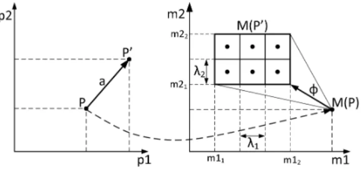
To tackle exploration accuracy, the metrics space is par-titioned according to a parameter−→λ defined for the explo-ration. −→λ is a vector of scalars that specifies the maximum width of a partition for each metric. Partitioning is used to divide large areas into smaller areas such as the maxi-mum error is defined byλ, given by the difference between the present value of the metrics (to be determined through simulation) and the centroid of the partition that best ap-proximates it. An example of an action on a parameter is illustrated in Figure1where actiona, applied toP, gener-atesP′

=τ(P, a). The metrics M(P′

) are evaluated from

Figure 1: An example of actions on P. The met-rics space is partitioned in 6 areas and centroids are illustrated with black dots

M(P) through domain knowledge Φ and results in an area included into h[m11, m12],[m21, m22]i. The area is

parti-tioned in six partition (whose centroids are depicted with black dots) according to−→λ.

The utility function (Ψ) has the utility property [20] and is a function of the metrics M. In a multi-objective explo-ration, metrics are combined in order to be able to enumer-ate the solutions. Ψ can be linear (w1m1+w2m2+...+wimi)

or exponential (mw1

1 +m w2

2 +...+m wi

i ). To obtain the pareto

curve, the exploration is performed in a multivariate envi-ronment, thus−W→={w1, w2, ...wi}must change during the

exploration in order to explore all the directions of the met-rics space. In a two-dimensional metmet-rics space, this can be achieved, i.e., using the scalarizing functionmα

1m (1−α) 2 with

αin [0,1].

The exploration is modeled as a MDP:

Definition _3. _{A MDP is a tuple}_{< S, A, T P , R >}_where: • S is the set of possible states describing a solution of

the DSE problem;

• A is the set of possible actions that can be applied on the states;

• T P:S×A→Π(S)is the state transition function as the probability density function for every state-action pair;

• R :S×A×S′

→ R is the expected reward for each state-action pair.

The behavior of the MDP is described with the Decision TreeD, a tree-based structure used to evaluate the various configurations. A nodes∈S inDrepresents a state of the system expressed by the tuplehP, Mi, whereP is a point in the parameters space and M a point in the metrics space. An edgee∈Eis defined as:

e=hsi, sj, a, T P(si, a, sj)i

and it represents the transition probability (given by the transition functionT P) from statesito statesjwhen action

ais applied.

Each partition identifies a new node in the decision tree, and the reward of the actions (R) is computed as the differ-ence between parent (Ψp) and child (Ψc) utility functions:

R= Ψp−Ψc (2)

For each partitionhs, a, s′

i, the probabilityT Pi(si, a, sk) is

computed as the number of times hs, ai ends in s′

when traversing the decision tree from root to leaf. The decision

(4)

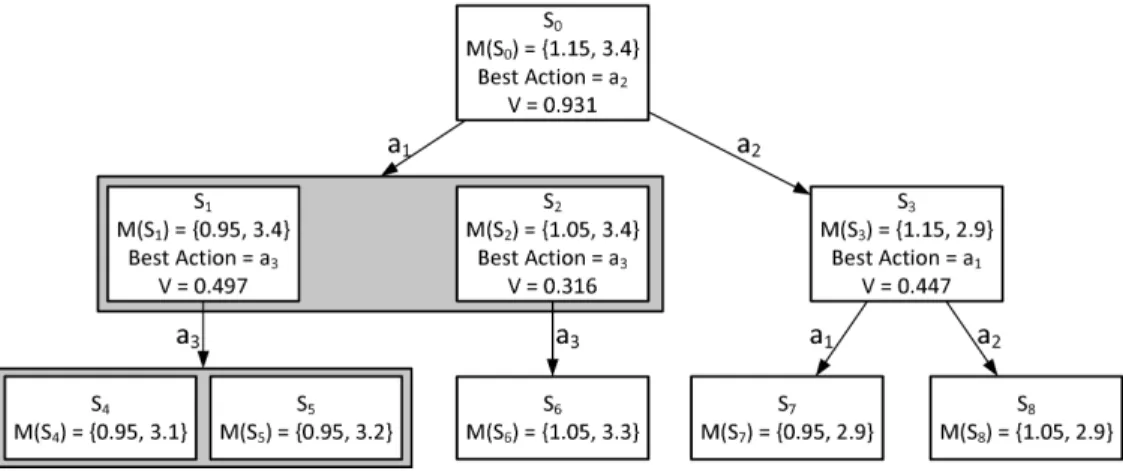
Figure 2: Example of a Decision Tree D. Cumulative return V is computed using the Value Iteration Algorithm (see Algorithm1)

tree is progressively built by iterating on the newly gener-ated nodes breadth-first, until either is not possible to ap-ply any other action on the leaf nodes or thel-th level is reached. During the creation ofD, in order to avoid useless exploration,opposite actions are included into a forbidden listsuch as they will not be applied. For example, if the ac-tionIncrease CPU frequencyis applied, the actionDecrease CPU frequency in included into the forbidden list since it voids the previous action.

An example of the Decision Tree D is shown in Figure

2. From the initial states0, two actions are applied (a1, a2)

resulting in three states (s1, s2, s3) wheres1 ands2 are two

partitions. Actionsa3anda1 are further applied on the

sec-ond level of the tree. For each state, metrics are associated; this example has two metrics that must be minimized. Re-wards estimate the benefits of the actions on Ψ and are used to guide the exploration to better solutions. To determine the reward of the actions, Value Iteration Algorithm (see Algorithm1) is used onD. For all the states in the tree and for all the available actions, the reward of an actionQ(s, a) is computed by adding the reward of choosing that action (R(s, a, s′

)) with the cumulative return on the destination node (V(s′

)) scaled byγ. γ is a scalar value (0≤ γ ≤1) used to control the influence of (expected) cumulative re-turns. Transition probability T P(s, a, s′

) is considered in the formula. In this specific example, V is computed by considering γ = 0.6 and the utility function m10−α+mα1

withα= 0.5. According to the metrics, the algorithm iden-tifies a2 as the best action in this situation; in fact, s7 is

optimal with respect to the given metrics. The new state is s3 and no simulation is required since no uncertainty is

detected here.

The overall exploration strategy is illustrated in Algo-rithm2. It starts (first step) by generating an initial con-figurationP0 (line5) – that can be identified randomly or

pseudo-randomly. Once P0 has been evaluated by

simula-tion and the initial states0has been generated (line6), the

set of states to be examined (S) is initialized (line7). Thesecond step of the algorithm solves the MDP. For each state in s, all possible actions are applied, generat-ing the configurations that differ from s0 by one

parame-ter (lines13-26). For all the generated configurations (ob-tained by applying a in si), sk metrics are partitioned, D

andT P(si, a, sk) are updated. The generation of the

Deci-Algorithm 1:Strategy Evaluation Algorithm 1 initializeV(s) = 0 2 repeat 3 forall thes∈S do 4 forall thea∈Ado 5 Q(s, a) = P s′∈S T P(s, a, s′ )[R(s, a, s′ ) +γV(s′ )] 6 end 7 V(s) = maxaQ(s, a) 8 end

9 untilstrategy converges;

sion Tree continues until no new states are available or the maximum depthlhas been reached. At this point (line27) the best value iteration algorithm [20] is applied and the best actions are updated onD.

The third step applies the best action of s0 in s0 to

get the set of reachable states (N S). At this point, three situations are possible:

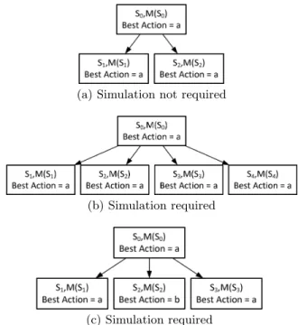
1. No Uncertainty: the action can lead to a single state. The action is determined with an accuracyλ and no simulation is necessary;

2. Uncertainty of the First Kind: the action leads to a set of states and the algorithm maps the same action to all of them. It means that, whichever state the system will end into, the same next action is chosen. In case the amount of states is below a given thresholdK, simulation is not required and parallel exploration will follow, otherwise simulation is required; K controls the amount of solutions to be explored and is used to tackle the scalability of the algorithm. Parallel explorations could evolve differently since they start from different partitions, thus they must be considered separately; 3. Uncertainty of the Second Kind: the action leads

to a set of states, but the algorithm maps two or more different actions on those states. In this situation, sim-ulation is needed to determine to which state the action really leads to.

Three examples of uncertainties are depicted in Figure3. In

3(a)an uncertainty of the first kind is detected and|N S|< Kthus simulation is not required. In3(b)an uncertainty of

(5)

Algorithm 2:Overall Exploration Strategy 1 Identify the configuration parameters−→P

2 Define the movement vectors Φ 3 num runs=0

4 repeat

5 Generate an initial configurationP0

6 sinit= Simulate(P0)

7 Initialize the set of states to be examinedS=sinit

8 repeat 9 depth = 0 10 resetD 11 get an elements0∈S, S=S−s0 12 s=s0 13 repeat 14 snew={} 15 forall thesiinsdo

16 forall thea applicable insido

17 applyainsicreating child nodessk

18 partitionskmetrics

19 updateD andT P(si, a, sk)

20 snew=snew+sk

21 addato forbidden action list ofsi

22 end

23 end

24 s=snew

25 depth++

26 untils=∅or depth == l;

27 Value Iteration Algorithm(D)

28 NS =τ(s0, best action(s0))

29 if |N S| ≥K or(∃si, sj∈NS: best action(si)6=

best action(sj) and i6=j)then

30 snext= Simulate(Ps0)

31 if snext∈/NS then

32 Error−→Restart From Line5

33 end 34 N S=snext 35 end 36 if convergency then 37 Simulate(Ps0) 38 else 39 S=S+N S 40 end 41 untilS=∅; 42 num runs++

43 untilnum runs≥MAXRUNS;

44 Change Utility Function 45 Repeat All

the first kind is detected but|N S| ≥K thus simulation is required. In3(c)simulation is required since an uncertainty of the second kind is detected.

In other terms, simulation is performed only if the car-dinality of N S (the amount of states reached by the best action) is above a given valueKor the actionabrings the system toa set of states and the Value Iteration Algorithm mapped different actions to each of those states. In case simulation resultssnextare not contained inN Sexploration

restarts from line5, otherwise N S is update with the real value snext. At this point the algorithm checks if

conver-gency has been reached (line 36); in the positive case, a

(a) Simulation not required

(b) Simulation required

(c) Simulation required

Figure 3: Uncertainties of First and Second Kind

withK= 3

simulation is performed (line 37) to get the real values of the metric of s0 (unless it has been previously simulated),

otherwise,Sis updated and the exploration continues. Step one, two and three are repeated until a maximum number of runs (MAXRUNS) has been performed.

In thelast step, the weights−→w of the utility function Ψ are updated (line44) and the algorithm is entirely repeated. It allows tochange the directionof the exploration in order to cope multi-objective optimizations. The algorithm stops when no more utility functions would be used.

In conclusion, the algorithm explores all the possible ac-tions for all the reachable states with an event horizon of l

to determine an optimal local action considering various se-quences of actions. The effectiveness of the approach strictly depends on the quality of the movement vectors; as the accu-racy of movement vectors increases, the amount of required simulations decreases. In fact, in the optimal case, move-ment vectors identify areas with size lower thanλ, thusNo Uncertainty is detected. In this case, assuming that move-ment vectors are accurate, simulation is required at the be-ginning (line6) and end (line37) only, thus simulations are minimized and exploration speed is maximized. In the worst case, non accurate movement vectors may conduct to Un-certainties of First (with |N S|> K) orSecond Kind, thus simulations are required at each step, leading to slower ex-plorations. More generally, to control the accuracy and the speed of the exploration (number of states in the MDP) two mechanisms have been identified:

• Control the minimum desired accuracy withλ.

It identifies the size of the partitions during the gen-eration of the Decision Tree; increasingλreduces the number of partitions (states), improving the evaluation speed, but it increases the approximation error;

• Define a good event horizon l, which determines the maximum depth of the Decision Tree. It limits the number of steps required to the creation/evaluation

(6)

of the MDP. Reducing l improves the speed of MDP evaluation since fewer states are generated into the de-cision tree D. On the other hand, the higher is lthe higher is the lookahead of the algorithm.

5. DOMAIN KNOWLEDGE DEFINITION

FOR IEEE 802.15.4 NETWORKS

The proposed approach requires movement vectors to guide the exploration to optimal solutions. In this sec-tion, we discuss a domain knowledge definition for the IEEE 802.15.4 MAC layer. The proposed MDP does not re-quire accurate movement vectors to operate [5], thus it is not required that the users give accurate models to use this methodology; moreover, movement vectors are reusable. However, the analysis proposed in this Section has two main goals: first, to show in practice how to build a set of domain-specific rules to exploit the potential of the MDP algorithm. Second, it provides a good characterization of one the most popular MAC protocols in WSNs, hence the proposed rules can be reused.

The IEEE 802.15.4 standard [3] has been introduced to satisfy energy requirements of emergent devices. The proto-col is quite common, thus the knowledge domain defined in this Section can be useful for future works. The results pre-sented here are based on the models prepre-sented in [12] [21] [11] [6] [9] [18]. IEEE 802.15.4 network is composed by a central node, called coordinator, and a set of nodes, called members. In IEEE 802.15.4, the coordinator is the head of the network and determines the structure of the communi-cation. In the standard, the communication is divided into sequential frames delimited by specific packets called bea-cons (Figure4). A frame is divided into an active and an inactive period, and the active part is further divided in two periods named Contention Active Period (CAP) and Con-tention Free Period (CFP). During the CAP, nodes access the channel by using the CSMA/CA protocol, while, during the CFP, the nodes access the channel using a time division protocol which slots, namely Guarantee Time Slots (GTS), are assigned by the coordinator by means of a policyFirst Come First Served(FCFS) [3].

The metrics of interests are Average Energy Consumption (E), to be minimized, and Percentage of Packets Received (P), to be maximized. The IEEE 802.15.4 is characterized by a certain amount of node and network parameters. For the sake of simplicity, we decide to restrict the analysis to four parameters: SuperframeOrder,BeaconOrder, en-ableCAPandrequestGTS. According to the state of the art, these parameters have considerable effects on the met-rics of interests, thus their optimization is important to the final design. In all the equations the following constraint

Figure 4: An example of the superframe structure (from [3])

must be satisfied:

(0≤P ≤100)∧(E≥0) (3)

In case the equation is not satisfied, P and E are set to the nearest value which satisfies the equation. I.e., ifP <0 then

P is set to zero. The next two sections presents in detail the movement vectors. In all the equations,EandPrepresents the actual value of the metrics while Eb and Pb represents their estimated (next) value.

5.1 Beacon Order and Superframe Order

Beacon Order (BO) and Superframe Order (SO) define the main structure of the superframe since they determine the distance between the beacons and the size of the active period. The ratio between SO and BO defines the duty cycle between active and inactive period. The overall effect of increasing BO and decreasing SO is similar, since both actions modify the duty cycle in the same way. Increasing BO or decreasing SO will halve the duty cycle, thus both E and P can be reduced by 2. Resulting movement vectors to actionsincrease BOanddecrease SOare:

b E= E 2, E (4) b P = P 2, P (5) On the other hand, actions that decrease BOand in-crease SOhave an opposite behavior, since duty cycle is doubled:

b

E= [E,2E] (6)

b

P= [P,2P] (7) All these actions can be applied if and only if the con-straint:

SO≤BO (8)

is satisfied. This constraint is imposed by the standard [3].

5.2 Guaranteed Time Slots

Each node requires a certain amount of GTS to the co-ordinator, according to therequestGTS parameter. The co-ordinator assigns the GTS according to the FCFS policy. It implies that if requested GTS are not designed properly, performances of the network dramatically decreases.

The maximum amount of available slots in slotted IEEE 802.15.4 is given by the following formula:

M =N SS−

_minCAP

BSD∗2F O

(9) where NSS is theNumber of Superframe Slots, minCAP is the minimum number of symbols in CAP and BSD is the Base Slot Duration.

The average amount of slots per node is equal to:

A= M

N (10)

and the overall amount of requested slots is equal to:

U=

N

X

i=0

(7)

where G(i) represents the value of requestGTS of node i. From [18] and experimental results, we notice that, increas-ing the GTS requests improves P and reduces E. P is im-proved because contention is reduced and E decreases since nodes wake-up are scheduled more efficiently in CFP with respect to CAP. In particular, when a GTS slot is allocated and few packets are in the buffer, the node sleeps during CAP and wake-ups just at the beginning of the GTS slot. In addition, since IEEE 802.15.4 uses a TDMA protocol dur-ing CFP, no additional energy is required to performCarrier Sense.

According to the FCFS policy, if GTS have been already allocated and it is not possible to satisfy the request, the request is rejected and the node is obliged to communicate into the CAP. GTS requests are rejected if the amount of requested GTS slots (Equation11) overcomes the maximum amount of slots in CFP (Equation9). Moreover, in order to balance GTS requests, the amount of GTS requests per node

n (G(n)) should not overcome the average GTS requests (Equation 10). The effect of increasing/decreasing GTS is limited to a single-slot of a single-node, so the value of P and E should be divided byN M to provide more accurate movement vectors.

Actionincrease requestGTSon node n results in:

b E= ( E− E N M, E ifU≤M∧G(n)≤A E, E+ E N M otherwise (12) b P= ( P, P+ P N M ifU ≤M∧G(n)≤A P− P N M, P otherwise (13)

On the other hand, action decrease requestGTShas the following movement vectors:

b E= ( E, E+ E N M ifU≤M∧G(n)≤A E− E N M, E otherwise (14) b P= ( P− P N M, P ifU ≤M∧G(n)≤A P, P+ P N M otherwise (15)

5.3 Enable CAP

Considering the enableCAP parameter, two actions are possible: activate and deactivate CAP. The overall effect of enabling CAP is the increase of energy consumption (due to CAP period) and an increase of packets received. Similarly to GTS, the action has an effect on a single node only, thus both E and P changes are scaled to N. Moreover, the higher is the amount of GTS requests of a node, the lower is the effect of activation/deactivation of CAP, so the metrics are divided by G(n)+1.

Differently from energy, packets received have a known behavior in caseG(n) is equal to zero. In fact, whenG(n) = 0 and CAP is not enabled, the amount of packets sent by a nodenis equal to zero, thus activating CAP whenG(n) = 0 has a increases the number of packets received (P

N, 100

N

); the deactivation of CAP when G(n) = 0 has the opposite effect. The movement vectors of the actionactivate CAP are: b E= E, E+ E N(G(n) + 1) (16) b P = ( P+P N, P+ 100 N ifG(n) = 0 h P, P+ P N(G(n)+1) i otherwise (17)

for the action deactivate CAP, the movement vectors are: b E= E− E N(G(n) + 1), E (18) b P = ( P−100 N , P− P N ifG(n) = 0 h P− P N(G(n)+1), P i otherwise (19)

5.4 Initial Points Selection

In the classical MDP, the set of initial points is randomly generated but, especially with large design spaces, the prob-ability to obtain bad (or even unfeasible) solutions is high. Therefore, the selection of the initial points can be guided by the model since, considering that the knowledge base has been already created to compute the actions, the same in-formation can be used to extract the initial points.

To define the rules for the selection of the initial points, we conduct several experiments on star networks with 4, 6 and 8 nodes with various packet rates (5, 15, 30, 50, 65, 80pkts

sec

) in order to cover a large set of applications. All the experiments where conducted with Castalia simulator [2] (see next Section). From the experimental results, we notice that assigning arequestGTS greater than the average (A), reduces the quality of the solution, so we suggest to create the initial population with a starting value of request-GTS randomly chosen in the interval [0, A]. In addition, a value of Beacon Order lower than 3 or greater than 12 does not usually provide good results, thus we generate the ini-tial solution with BO included into [3,12]. Another aspect concerns the duty cycle (SO

BO); good solutions usually have a

duty cycle included into [0.25,0.85] in all the configurations. Summarizing, to determine the initial points, we propose to generate the set of initial points in such a way:

   0≤G(n)≤A ∀n∈N 3≤BO≤12 0.25≤ SO BO ≤0.85 (20) so that these constraints are all satisfied.

Experimental results in the next Section show that a con-siderable improvement on search efficiency is obtained if ini-tial points are determined using this technique.

6. EXPERIMENTAL RESULTS

This Section presents two sets of experiments to validate the proposed approach. The solutions were evaluated with Castalia [2], a popular simulator for Wireless Sensor Net-works and Body Area NetNet-works, based on the OMNeT++ framework [22]. The design space for all the experiments is presented in Table2. The design space has been explored in four different scenarios described in Table3. These scenarios have been chosen in order to cover a large set of applications (i.e. Body Area Networks).

Since the cardinality of the design space is extremely high in all the scenarios, the optimal Pareto curve cannot be ex-tracted with an exhaustive search, thus it has been obtained running all the exploration algorithms for 3000 iterations (solutions) for 20 iterations each. The distance between the

(8)

Table 2: Explored Design Options for the Experi-mental Results

Parameter From To

Beacon Order 1 14

Frame Order 1 14

Enable Cap false true

requestGTS 0 6

Table 3: Experimental Scenarios

Num of Packet Rate Size of the

Nodes (Pkts/Sec) Design Space

Scen. 1 4 30, 65, 80 7.5∗106

Scen. 2 6 15, 40, 60 1.4∗109

Scen. 3 8 5, 15, 30 2.9∗1011

Scen. 4 10 5, 10, 15 5.6∗1013

Pareto sets have been compared using theAverage Distance from Reference Set(ADRS) [17]. The ADRS is usually mea-sured in terms of percentage and should be minimized.

6.1 Evaluation of the Proposed Algorithm

The first set of experiments aims at evaluating the im-provements achieved thanks to the tailoring of the standard MDP technique to the WSN field. In particular, Table4

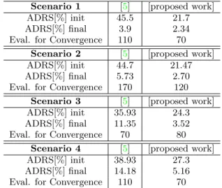
presents a comparison between the standard implementa-tion of the MDP algorithm and the one proposed within this work. The experimental results shown in Table 4 demon-strate that the ADRS of the initial points of the proposed algorithm is considerably lower than the ones obtained with [5]. This advantage makes it possible to increase the overall performance of the algorithm, so that the ADRS of the final solutions found by our algorithm is always lower than the ones obtained with [5]. In addition to this, the proposed algorithm is able to converge with a lower number of eval-uations, except for Scenarios 3 and 4, where the algorithm presented in [5] often falls in local minima (as shown by the quite high ADRS of the solutions found by the algorithm).

A critical aspect of the standard MDP algorithm is its scalability. In order to analyze this factor, we suggest to handle uncertainties of the first kind with simulations only if the number of states (|N S|) is larger than a given thresh-old K. To evaluate the effect of K on the exploration speed

1 10 100

3 5 15 30

Num. of Parallel Explorations

Average Number of Generated States

K=inf. K=10 K=5 K=2

Figure 5: Number of parallel explorations with dif-ferent values of K (K=inf. refers to the original al-gorithm). The average number of generated states

depends on the chosenλand movement vectors’

ac-curacy

Table 4: Comparison between original and proposed implementation of the MDP

Scenario 1 [5] [proposed work]

ADRS[%] init 45.5 21.7

ADRS[%] final 3.9 2.34

Eval. for Convergence 110 70

ADRS[%] init 44.7 21.47

ADRS[%] final 5.73 2.70

ADRS[%] init 35.93 24.3

ADRS[%] final 11.35 3.52

ADRS[%] init 38.93 27.3

ADRS[%] final 14.18 5.16

we perform several experiments with different values of K; Scenario 2 has been chosen as reference example for this analysis. We vary the values ofλsuch as the average num-ber of generated states for each action is between 3 (higher

λ) and 30 (lowerλ). Figure 5illustrates the average num-ber of parallel explorations for different values of K with respect to the average number of states for each step. The bigger is K, the higher is the amount of parallel (indepen-dent) explorations. However, the effective exploration time is not directly correlated with the amount of parallel explo-rations. Figure6illustrates the average amount of time (in minutes) required for the exploration with different values of K. Although the number of parallel evaluations increases with both K and the number of generated states, the overall time behaves differently. In fact, for small values of gen-erated states, K=5 performs better then K=2 even if the amount of parallel exploration is bigger. However, for high values of generated states (i.e. 30), K=2 performs better. K=inf have no better performances in all the situations; it confirms that a bound on the generated states increase the exploration’s speed. Moreover, we notice that exploration efficacy (ADRS and convergence speed) is not affected byK

since it strictly depends onλ, thus it is suggested to tune K such that the exploration time is minimized.

1 10 100 1000

3 5 15 30

Avg. Exploration Time [min]

Average Number of Generated States

K=inf. K=10 K=5 K=2

Figure 6: Amount of time (in minutes) required for the exploration with different values of K (K=inf. refers to the original algorithm). The average num-ber of generated states depends on the chosenλand movement vectors’ accuracy

(9)

0 2 4 6 8 10 12 14 0 50 100 150 200 250 300 350 400 ADRS [%] Number of Evaluations mdp nsgaii pma mosa

Figure 7: ADRS per Number of Evaluations in Sce-nario 1 0 2 4 6 8 10 12 14 0 50 100 150 200 250 300 350 400 ADRS [%] Number of Evaluations mdp nsgaii pma mosa

Figure 8: ADRS per Number of Evaluations in Sce-nario 2

The proposed algorithm is able to reduce/control the ex-ponential growth of the number of parallel executions with respect to the original approach presented in [5] (where the threshold K has not been defined). Then, in addition to improving the quality of the final solution, the proposed ap-proach is also able to reduce the number of explorations to be performed, thus reducing the computational costs and time required by the algorithm itself.

6.2 ADRS and Number of Evaluations

The second set of experiments compares the proposed MDP with three state-of-the-art multiobjective optimiza-tion algorithms: controlled non-dominated sorting genetic algorithm (NSGA-II), Pareto memetic algorithm (PMA) and multiple objective simulated annealing (MOSA). The MOMHLib++ [1] library was used as a reference implemen-tation of these algorithms. In order to ensure a fair compar-ison, all the algorithms exploits the technique described in Section5.4to generate the initial points.

Each configuration of all the optimization algorithms has been executed for 20 times in the four scenarios and the average ADRS has been evaluated. We compute the ADRS every 5 evaluations in order to understand its trend with respect to the number of evaluations. The results of these experiments are presented in Figure7(Scenario 1), Figure8

(Scenario 2), Figure9(Scenario 3) and Figure10(Scenario 4), which show that MDP is able to reach a low ADRS (below 5%) using less than 40 evaluations, while the other algorithms require from 100 to almost 300 evaluations to reach the same objective. This is a reduction of 60-87% in the number of required simulations. The time required to evaluate a single solution varies from 7 (Scenario 1) to 18 minutes (Scenario 4), that implies an exploration time of almost 5 hours for MDP and 12-36 hours for others in

0 2 4 6 8 10 12 14 0 50 100 150 200 250 300 350 400 ADRS [%] Number of Evaluations mdp nsgaii pma mosa

Figure 9: ADRS per Number of Evaluations in Sce-nario 3 0 2 4 6 8 10 12 14 0 50 100 150 200 250 300 350 400 ADRS [%] Number of Evaluations mdp nsgaii pma mosa

Figure 10: ADRS per Number of Evaluations in Sce-nario 4

Scenario 1, 12 hours for MDP and 30-60 hours for others in Scenario 4. These numbers illustrate the practical efficacy of the proposed approach for real-life WSN designs exploration and optimization.

As design space cardinality increases, the identification of the Pareto curve is more difficult, thus exploration efficiency decreases. It is interesting to notice that the reduction of effectiveness of MDP is considerably lower than the other algorithms (See Table 5). These results encourage the use of such algorithm on large design spaces.

During the Design Space Exploration, optimization algo-rithms should be run several times in order to guarantee the quality of the identified Pareto curve. Analyzing the standard deviation of the ADRS on the independent runs, we observed that standard deviation on MDP is the low-est. Table6summarized the computed standard deviations. A low standard deviation implies that the optimization al-gorithm requires few repeats to guarantee the quality; it

Table 5: Final ADRS of search Algorithms

MDP NSGA-II PMA MOSA

Scenario 1 2.34 1.42 0.83 1.43

Scenario 2 2.70 2.88 0.78 2.20

Scenario 3 3.52 6.52 4.76 5.36

Scenario 4 5.16 9.55 8.78 7.32

Table 6: Standard Deviation of ADRS

MDP NSGA-II PMA MOSA

Scenario 1 0.34 1.20 1.01 1.34

Scenario 2 0.55 2.56 1.94 1.91

Scenario 3 0.64 2.44 2.38 2.81

(10)

further reduces the overall time required for Design Space Exploration.

7. CONCLUDING REMARKS

This paper has presented a technique to reduce the amount of simulations necessary to obtain the Pareto set of the design space exploration of Wireless Sensor Networks. The proposed technique uses models as soon as they pro-vide an acceptable accuracy and simulates only when it is needed. The knowledge domain about slotted IEEE 802.15.4 has been extracted from the models of the state of the art. Experimental results have shown that proposed algorithm significantly improves the efficiency and scalability with re-spect to the classical algorithm. To confirm the efficacy of the technique, we also compared the proposed approach with semi-random algorithms such as NSGA-II, PMA and MOSA. Experimental results have shown that MDP reduces the number of simulations required to converge (ADRS lower than 5%) from 60 to 87%. This reduction is more effective as the cardinality of the design space increases, making it an effective approach for the design space exploration of WSNs.

8. REFERENCES

[1] MOMH: multiple objective meta heuristics [online]. available: http://home.gna.org/momh/.

[2] OMNET++ castalia simulator, [Online] http://castalia.npc.nicta.com.au/.

[3] IEEE standard for information technology. 802.15.4 standard specification, 2006.

[4] L. S. Bai, R. P. Dick, P. H. Chou, and P. A. Dinda. Automated construction of fast and accurate system-level models for wireless sensor networks. In Design, Automation & Test in Europe Conference & Exhibition (DATE), 2011, pages 1–6. IEEE, Mar. 2011.

[5] G. Beltrame, L. Fossati, and D. Sciuto. Decision-Theoretic design space exploration of multiprocessor platforms.IEEE Transactions on Computer-Aided Design of Integrated Circuits and Systems, 29(7):1083–1095, July 2010.

[6] C. Buratti. A mathematical model for performance of IEEE 802.15.4 beacon-enabled mode. InProceedings of the International Conference on Wireless

Communications and Mobile Computing: Connecting the World Wirelessly, IWCMC ’09, pages 1184–1190, New York, NY, USA, 2009. ACM.

[7] K. P. Ferentinos and T. A. Tsiligiridis. Adaptive design optimization of wireless sensor networks using genetic algorithms.Computer Networks,

51(4):1031–1051, Mar. 2007.

[8] O. Goussevskaia, R. Wattenhofer, M. M. Halldorsson, and E. Welzl. Capacity of arbitrary wireless networks. InIEEE INFOCOM 2009, pages 1872–1880. IEEE, Apr. 2009.

[9] J. He, Z. Tang, H. Chen, and Q. Zhang. An accurate and scalable analytical model for IEEE 802.15.4 slotted CSMA/CA networks.IEEE Transactions on Wireless Communications, 8(1):440–448, Jan. 2009. [10] Z. He, J. Eggert, W. Cheng, X. Zhao, J. Millspaugh,

R. Moll, J. Beringer, and J. Sartwell. Energy-aware portable video communication system design for wildlife activity monitoring.Circuits and Systems Magazine, IEEE, 8(2):25 –37, 2008.

[11] M. Kohvakka, M. Kuorilehto, M. Hännikäinen, and T. D. Hämäläinen. Performance analysis of IEEE 802.15.4 and ZigBee for large-scale wireless sensor network applications. InPerformance evaluation of wireless ad hoc, sensor and ubiquitous networks, pages 48–57, New York, NY, USA, 2006. ACM.

[12] G. Lu, B. Krishnamachari, and C. S. Raghavendra. Performance evaluation of the IEEE 802.15.4 MAC for low-rate low-power wireless networks. In2004 IEEE International Conference on Performance, Computing, and Communications, pages 701– 706. IEEE, 2004. [13] E. Meshkova, J. Riihijarvi, A. Achtzehn, and

P. Mahonen. Exploring simulated annealing and graphical models for optimization in cognitive wireless networks. InIEEE Global Telecommunications Conference, 2009. GLOBECOM 2009, pages 1–8. IEEE, Dec. 2009.

[14] A. Munir and A. Gordon-Ross. An mdp-based application oriented optimal policy for wireless sensor networks. InProceedings of the 7th IEEE/ACM international conference on Hardware/software codesign and system synthesis, CODES+ISSS ’09, pages 183–192, New York, NY, USA, 2009. ACM. [15] S. Nabar, J. Walling, and R. Poovendran. Minimizing

energy consumption in body sensor networks via convex optimization. InBody Sensor Networks (BSN), Int. Conf. on, pages 62 –67, June 2010.

[16] M. Nabi, M. Blagojevic, T. Basten, M. Geilen, and T. Hendriks. Configuring multi-objective evolutionary algorithms for design-space exploration of wireless sensor networks. InProceedings of the 4th ACM workshop on Performance monitoring and measurement of heterogeneous wireless and wired networks, PM2HW2N ’09, pages 111–119, Tenerife, Canary Islands, Spain, 2009. ACM.

[17] G. Palermo, C. Silvano, and V. Zaccaria. ReSPIR: a response Surface-Based pareto iterative refinement for Application-Specific design space exploration.

Computer-Aided Design of Integrated Circuits and Systems, IEEE Transactions on, 28(12):1816 –1829, Dec. 2009.

[18] P. Park, C. Fischione, and K. H. Johansson. Performance analysis of GTS allocation in beacon enabled IEEE 802.15.4. In6th Annual IEEE

Communications Society Conference on Sensor, Mesh and Ad Hoc Communications and Networks, 2009. SECON ’09, pages 1–9. IEEE, June 2009.

[19] M. A. Pasha, S. Derrien, and O. Sentieys. System-Level synthesis for wireless sensor node controllers.ACM Transactions on Design Automation of Electronic Systems, 17(1):1–24, Jan. 2012.

[20] S. Russel and P. Norvig.Artificial Intelligence: Modern Approach. 1st ed. englewood cliffs, NJ: prentice hall edition, 1995.

[21] N. F. Timmons and W. G. Scanlon. Analysis of the performance of IEEE 802.15.4 for medical sensor body area networking. pages 16– 24. IEEE, Oct. 2004. [22] A. Varga. The OMNET++ discrete event simulation

system. InProceedings of the European Simulation Multiconference, pages 319–324. SCS – European Publishing House, 2001.