AUSTRALIA
DEPARTMENT OF ECONOMETRICS
AND BUSINESS STATISTICS
Local Linear Forecasts Using Cubic Smoothing Splines
Rob J. Hyndman, Maxwell L King, Ivet Pitrun and Baki Billah
splines
Rob J. Hyndman, Maxwell L. King, Ivet Pitrun, Baki Billah 27 August 2002
Abstract: We show how cubic smoothing splines fitted to univariate time series data can be used to obtain local linear forecasts. Our approach is based on a stochastic state space model which allows the use of a likelihood approach for estimating the smoothing parameter, and which enables easy construction of prediction intervals. We show that our model is a special case of an ARIMA(0,2,2) model and we provide a simple upper bound for the smoothing parameter to ensure an invertible model. We also show that the spline model is not a special case of Holt’s local linear trend method. Finally we compare the spline forecasts with Holt’s forecasts and those obtained from the full ARIMA(0,2,2) model, showing that the restricted parameter space does not impairforecast performance.
Key words: ARIMA models, exponential smoothing, Holt’s local linear forecasts, maximum likelihood estimation, nonparametric regression, smoothing splines, state space model, stochastic trends.
JEL classification numbers: C13, C14, C22, C53.
∗Department of Econometrics and Business Statistics, Monash University, Clayton, Victoria 3800.
Cor-respondence to [email protected].
1 Introduction
Suppose we observe a univariate time series{yt},t= 1, . . . , n, with non-linear trend. We are interested in forecasting the series by extrapolating the trend using a linear function estimated from the observed time series.
Linear trend extrapolation is very widely used and performs relatively well in prac-tice. For example, Makridakis & Hibon (2000), Assimakopoulos & Nikolopoulos (2000), and Hyndman & Billah (2002) discuss the excellent performance of linear trend methods in the M3-competition. In this paper, we discuss a method for local linear extrapolation of a stochastic trend based on cubic smoothing splines.
For equally spaced time series, a cubic smoothing spline can be defined as the func-tion ˆf(t) which minimises
n X t=1 (yt−f(t)) 2 +λ Z S[f 00 (u)]2du (1.1)
over all twice differentiable functions f on S where [1, n] ⊆ S ⊆ IR. The smooth-ing parameter λ is controlling the “rate of exchange” between the residual error described by the sum of squared residuals and local variation represented by the square integral of the second derivative of f. For a given λ, fast algorithms for computing ˆf(t) are described by Green and Silverman (1994). Large values of λ give ˆf(t) close to linear while small values of λ give a very wiggly function ˆf(t). In practice, λ is not generally known.
The solution to (1.1) consists of piecewise cubic polynomials joined at the times of observation, t = 1,2, . . . , n. Furthermore, the solution has zero second derivative at t = n. Therefore, an extrapolation of ˆf(t) for t > n is linear. The linear extrapolation of ˆf(t) provides our point forecasts.
We derive a new method for computing prediction intervals for these forecasts, utilizing a stochastic model formulation due to Wahba (1978) and Wecker and Ansley (1983). We also provide a new method for estimating the smoothing parameter λ.
Seasonally adjusted beer production (megalitres) 1970 1980 1990 2000 350 400 450 500 550
Figure 1: Cubic spline forecasts of Australian quarterly beer production (seasonally ad-justed) for September 2002 – June 2005, with 80% prediction intervals. The line through
the historical data show the fitted cubic spline fˆ(t); the forecasts are obtained by a
lin-ear extrapolation of fˆ(t); the prediction intervals are obtained from the state space model
described in Section 2. Here λ= 232.2.
Figure 1 gives an example of our forecast procedure applied to seasonally adjusted Australian quarterly beer production (March 1965 – June 2002). The fitted spline curve is shown along with the associated linear forecast function and 80% prediction intervals. The methodology provides a smooth historical trend, a linear forecast function and prediction intervals.
Forecasts are usually made using models which give most weight to recent obser-vations, and negligible weight to the distant past. This means that the smoothing parameter λ should not be too big for forecasting purposes. We make this explicit by finding the bounds on λrequired for our model to be invertible. (Specifically, we find that λ <1.640519n3
.)
Some linear forecast methods assume there is an underlying linear trend (e.g., a random walk with constant drift). We do not make this assumption. Our forecast function is linear, but the underlying trendf(t) is allowed to be non-linear. Further,
the possible future changes in trend direction are accommodated in our prediction intervals.
An alternative approach to local linear forecasting is to allow a deterministic non-linear trend. This is the approach followed by Nottingham and Cook (2001), for example. We prefer the stochastic trend approach as it allows the uncertainty in the trend to be explicitly allowed for in the measures of forecast uncertainty. A hybrid approach, combining both deterministic and stochastic trends, is provided through SEMIFAR models (see Beran and Ocker, 1999; and Beran and Feng, 2002).
Other local linear forecast models with stochastic trends include an ARIMA(0,2,2) model, Harvey’s (1989) local linear growth model and the AN model of Hyndman, Koehler, Snyder & Grose (2002) which underlies Holt’s (1957) linear trend method. In fact, these are all connected—Harvey’s model is asymptotically equivalent to the AN model, and the AN model is a reparameterization of an ARIMA(0,2,2) model. Our paper is structured as follows. Section 2 describes the stochastic model formu-lation for the cubic smoothing spline forecasts and Section 3 shows how to estimate the smoothing parameter. Simple expressions for obtaining point forecasts and pre-diction intervals are given in Section 4. In Section 5 we discuss the relationship between our model, an ARIMA(0,2,2) model and a state space model underlying Holt’s linear trend forecasts. These relationships enable us to obtain the maximum bound for the smoothing parameterλto ensure invertibility. Finally, in Section 6 we compare the forecasting performance of our model with other local linear forecasting models.
2 State space model
The definition of cubic smoothing splines given in Section 1 provides suitable point forecasts, but does not allow estimation of forecast uncertainty. To that end, we shall use the stochastic process formulation proposed by Wahba (1978) and developed in subsequent work of Wecker and Ansley (1983). We present Wecker and Ansley’s
state space model in the special case of cubic smoothing splines applied to equally spaced data.
First, we transform the observation time space to [0,1] by defining the transformed observation times as {t1, . . . , tn} where ti = i/n. Note that this transformation means that λ is rescaled also. Our transformed value of λ isλ∗ =n−3λ.
Then, for i= 1,2, . . ., define
g(ti) =τ
Z ti
0 (ti−u)dW(u)
where τ >0 and W(u) is a standard Wiener process. Also let
ui =τ Z ti ti−1 (ti−u)dW(u) W(ti)−W(ti−1) and αi = g(ti)−g(t1) τ(W(ti)−W(t1)) .
Then we assume Yi satisfies the state space model
Yi = s0iβ+ (1,0)αi+ei, (2.1)
αi = Tiαi−1+ui, i= 1, . . . , n (2.2)
where β = (β0, β1)0 is normally distributed with zero mean and covariance matrix
cI, Ti = 1 i/n 0 1 ,
ei are iidN(0, σ2) and si = (1, ti)
0
. The starting condition isα0 = (0,0) 0
. The state
αi−1 is assumed independent of ui.
Wahba (1978) showed that lim c→∞E (s
0
iβ+ (1,0)αi |Y1, . . . , Yn) (2.3)
is the cubic smoothing spline ˆf(t) with λ∗ = σ2/τ2. Thus ˆf(t) is the mean of Yt,
recursions to the state space model (2.1) and (2.2). Furthermore, we can also obtain forecast variances in this way.
However, a more direct approach is possible using a matrix formulation of the model. Let Y = (Y1, . . . , Yn)0, e= (e1, . . . , en)0 and g = (g(t1), . . . , g(tn))0. Then
Y = Sβ+g+e (2.4)
where the ith row of S iss0
i.
Proposition 1 Let Y be given by (2.4). ThenY is normally distributed with mean
0 and covariance matrix
Ω =σ2
(cSS0+λ−1
∗ Σ +In)
where c has been rescaled and whereΣ is symmetric with the (j, k)th element on or above the diagonal given by
Σjk=σ2 n−3 j2 (3k−j)/6, k ≥j. That is Σ = σ 2 n−3 6 2 5 8 · · · 3n−1 5 16 28 ... 8 28 54 ... . .. ... 3n−1 · · · · · · 2n3 .
We provide a proof for this result in the Appendix.
We shall use the stochastic formulation given by (2.4) and Proposition 1 to obtain point forecasts and prediction intervals.
3 Estimation
Estimates of the smoothing parameter λ∗ can be obtained by maximizing the
like-lihood function of the model which is given by `(λ∗ |Y) =|Ω|
−1/2
(Y0Ω−1
Y)−n/2
. (3.1)
Let P be the upper-triangular matrix from the Choleski decomposition of σ2
Ω−1
. (Note that P depends only on λ∗.) Then, we can write
|Ω|−1/2 = σ−1 |P| (3.2) and (Y0Ω−1 Y)−n/2 = σn(Y∗0 Y∗)−n/2 =σn n X i=1 w2 i −n/2 (3.3) where Y∗
= PY and wi is the ith element of Y∗. Using (3.1)–(3.3), the log-likelihood is given by
log`(λ∗ |Y) = (n−1) logσ+ log|P| −
n 2 log n X i=1 w2 i . (3.4)
Thus we can estimate λ∗ by maximizing
log|P| − n 2log n X i=1 w2 i .
This is a new method for selecting a bandwidth for smoothing splines, although it is similar in spirit to the likelihood-based method of Wecker and Ansley (1983). (Our method is much faster as we do not need to iteratively apply GLS estimation or the Kalman filter.)
4 Prediction
We now wish to use the fitted model to predict the next n0 observations. We write
them as then0-vectorY0 =S0β+g0+e0whereY0 = [Yn+1, . . . , Yn+n0]
0
andg0,e0 are
Σ0as the symmetricn0×n0matrix with (j, k)th elementσ 2
n−3
(n+j)2
(2n+3k−j)/6 for k ≥j. It is assumed that Y0 has the same properties as the observed vector Y.
Then the variance-covariance ofY0 can be written as Ω0 =σ2(cS0S00 +λ −1
∗ Σ0+In0).
To derive the best linear unbiased predictor for Y0 and the variance-covariance
matrix of the associated prediction error, we first combine past and future values of {Yt}to obtain Z = [Y0,Y00]
0
with covariance matrix
E[ZZ0] = Ω U U0 Ω0 =σ 2 (cS1S 0 1+λ −1 ∗ Σ1+In+n0)
whereS1 and Σ1 are constructed analogously toS,S0, Σ and Σ0. Then, using
stan-dard results for conditional expectations of multivariate normal random variables (e.g., Rao, 1973, section 8a), we obtain
E[Y0 |Y] = U 0 Ω−1 Y (4.1) and Var[Y0 |Y] = Ω0−U 0 Ω−1 U. (4.2)
Equations (4.1) and (4.2) allow point forecasts and associated prediction intervals to be easily computed. In particular, the h-step ahead point forecast ˆYn+his thehth element of U0
Ω−1
Y, and its variance vh is the hth diagonal element of the matrix Ω0−U0Ω−1U. Since Yt is assumed normal, prediction intervals can be constructed
from these first two moments in the usual way. A 95% prediction interval is given by ˆYn+h±1.96√vh.
Note that these results assume that c, λ∗ and σ2 are known. In reality, c is any
sufficiently large number (in the empirical calculations described in this paper we use c= 100), and the parameterλ∗ can be estimated using the procedure described
in Section 3. To estimate σ2
, we first calculate one-step forecasts ˆYt and associated “variances”vt from (4.1) and (4.2) plugging in σ2
= 1. This has no effect on the forecast means, but the forecast variances will be incorrect by a factor ofσ2
. Soσ2
as ˆ σ2 = n X t=1 (Yt−Yˆt)2/vt.
5 Comparisons with other approaches
The spline model described above gives local linear forecasts based on a stochastic trend. We now explore connections between this model and other models which also have stochastic trends and produce local linear forecast functions.
In particular, we look at the range of values for λ which will lead to an invertible model. Invertibility is a desirable property of a forecasting model because we want to avoid models where the distant past has a non-negligible effect on the present.
5.1 ARIMA(0,2,2) models
It is known (see Wecker and Ansley, 1983) that the cubic spline state space model described in Section 2 is equivalent to an ARIMA(0,2,2) model with some restrictions on parameters. However, no-one seems to have explicitly worked out the connection, or the implications it has for forecasting with the cubic spline model.
We define the ARIMA(0,2,2) model as
Yt−2Yt−1+Yt−2 =εt−θ1εt−1−θ2εt−2
where {εt}is a Gaussian white noise process with variance σ2ε. For invertibility, we also require |θ2| <1, θ2 −θ1 < 1 and θ2+θ1 < 1 (Box, Jenkins & Reinsell, 1994).
Then the ARIMA(0,2,2) forecast function is ˆYn+h =`n+bnh where `n =Yn−θ2eˆn and bn=Yn−Yn−1+θ1eˆn+θ2(ˆen+ ˆen−1). (Here, ˆej denotes the jth residual.) Now Brown and de Jong (2001) show that the cubic spline model can be written as an ARIMA(0,2,1) process observed with error:
Yt =Xt+ηt, (1−B)
2
where ψ = 2 −√3, (X1, X2 −X1) is fully diffuse, and ηt and ξt are uncorrelated white noise series with means zero and variances σ2
and τ2
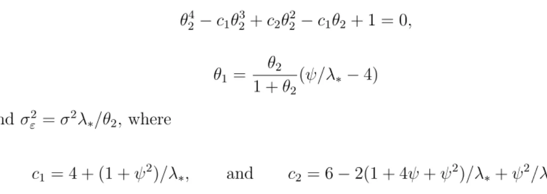
respectively. It is easy to show this is equivalent to an ARIMA(0,2,2) model with θ2 obtained by solving
the following quartic equation: θ4 2 −c1θ 3 2+c2θ 2 2 −c1θ2+ 1 = 0, θ1 = θ2 1 +θ2 (ψ/λ∗−4) and σ2 ε =σ 2 λ∗/θ2, where c1 = 4 + (1 +ψ 2 )/λ∗, and c2 = 6−2(1 + 4ψ+ψ 2 )/λ∗+ψ2/λ2∗.
Numerical calculations show that the above quartic equation has at most one root which gives an invertible solution, and that an invertible solution is obtained if and only if 0 < λ∗ <1.640519. Figure 2 shows the values ofθ1 and θ2 as functions of λ∗.
In the original time space (where observation times are 1,2, . . . , n), the upper bound on λ is 1.640519n3
. This upper bound on λ should be imposed whenever the spline model is used for forecasting purposes. If the model is simply used to describe the
0.0 0.5 1.0 1.5 −0.6 −0.4 −0.2 0.0 0.2 λ* ARIMA parameters θ1 θ2
Figure 2: The relationship between the ARIMA parametersθ1 andθ2 and the cubic spline
historical trend, invertibility is not relevant and so the bound need not be imposed. Note that the range of ARIMA(0,2,2) models that can be fitted in this way is greatly restricted, and that a wider range of models with linear forecast functions can be obtained by fitting a general ARIMA(0,2,2) model. In fact, Box, Jenkins & Reinsel (1994) show that all ARIMA(p,2,q) have forecast functions which areasymptotically
linear (the “eventual forecast function”), and that the forecast function is exactly
linear if and only if p= 0 andq≤2.
5.2 Holt’s local linear forecasts
Holt’s local trend method has been used in forecasting for many decades and it has proved remarkably versatile and useful. Point forecasts (see, e.g., Makridakis, Wheelwright and Hyndman, 1998, p.158) are given by ˆYn+h = `n+bnh where `n and bn are computed recursively as follows:
`t = αYt+ (1−α)(`t−1+bt−1) (5.1)
bt = β(`t−`t−1) + (1−β)bt−1 (5.2)
for t = 2, . . . , n. Starting values for these recursions are often set to `1 = Y1 and
b1 =Y2−Y1, although we choose the starting values optimally (see below).
The unobserved components `t and bt represent the level and slope of the series at time t and α and β are constants. We normally restrict the parameters such that 0≤α≤1 and 0≤β≤1.
Recently, Hyndman, Koehler, Snyder & Grose (2002) (hereafter HKSG) provided a general modelling framework for exponential smoothing methods, including Holt’s method. This enables the forecasts to be obtained from a state space model, thus providing facilities for maximum likelihood estimation, calculation of prediction in-tervals, etc. HKSG actually provide two state space models for Holt’s method, which give identical point forecasts but have different properties for high forecast moments. In this paper, we only consider the additive error version.
The model can be written as follows:
Yt = `t−1 +bt−1+εt `t = `t−1 +bt−1+αεt bt = bt−1 +αβεt
where `t denotes the level at time t, bt denotes the slope of the trend at time t, and εt is a Gaussian white noise process with zero mean and variance σ2. We estimate the parameters α and β and the initial state vector (`0, b0)
0
by maximizing the conditional likelihood as described in HKSG.
Hyndman, Koehler, Ord and Snyder (2001) show that the forecast mean of this model is identical to Holt’s local trend forecast and the forecast variance of the model is vh =σ2 h 1 +α2 (h−1)n1 +βh+ 1 6β 2 h(2h−1)o i.
Using this expressions, prediction intervals can be constructed in the usual way.
The above state space model underlying Holt’s method is equivalent to an ARIMA(0,2,2) model where α = θ2 + 1 and β = (1−θ1 −θ2)/(1 +θ2). In theory, the parameter
space for (α, β) could be taken as the whole invertible region for the ARIMA model (in which case we would have 0< α <2 and 0< β <4/α−2). However, it is usual to restrict the space further and require 0 < α < 1 and 0 < β < 1 which leads to more interpretable models.
However, for the spline model, we found that θ2 > 0. Therefore, α > 1 which
means that the spline model falls outside the usual range of parameters considered for Holt’s method. (We also found that β >1 whenλ∗ >0.14514.)
This means that Holt’s method and the cubic spline model are both special but non-overlapping cases of the ARIMA(0,2,2) model.
6 Empirical comparison of models
Given that the cubic spline model is a special case of an ARIMA(0,2,2) model, it is interesting to see if the restricted parameter space results in poorer forecasting performance. We will also compare the forecasts from Holt’s method based on a different and mutually exclusive subset of the parameter space of the ARIMA(0,2,2) model.
We compare the three models by applying them to the 645 annual series which were part of the M3 forecasting competition (Makridakis & Hibon, 2000). For each series, six observations were withheld at the end of the series for comparisons. The remaining observations were used for estimation of parameters.
For each series, we estimate the parameters using likelihood methods. We use the methods described in Sections 3 and 5.2 for the spline model and the state space model underlying Holt’s method, and for the full ARIMA model we use the exact likelihood method of Gardner, Harvey and Phillips (1980) as implemented in the ts library distributed with R 1.5.1.
Then each model is used to forecast the remaining six observations in the series. The forecasts are compared by computing the Mean Absolute Percentage Error (MAPE) averaged across all series and the Coverage Percentage (CP) of the (nominally) 95% prediction intervals computed over all series.
As a further comparision, we also applied the local linear method of Nottingham and Cook (2001), although this assumed a deterministic trend rather than a stochastic trend.
The results are given in Tables 1 and 2 and highlight some interesting similarities and differences between methods.
Forecast horizon Method h= 1 h= 2 h= 3 h= 4 h= 5 h= 6 Spline 9.8 23.0 26.8 32.0 37.6 41.9 ARIMA(0,2,2) 8.6 21.6 26.9 30.3 35.9 37.8 Holt 11.0 23.3 25.8 29.1 32.2 36.0 Local linear 11.8 23.1 26.3 28.4 32.6 36.9
Table 1: Mean Absolute Percentage Error for each model, computed by averaging the absolute percentage error across all 645 annual series.
Forecast horizon Method h= 1 h= 2 h= 3 h= 4 h= 5 h= 6 Spline 86.4 81.9 77.2 76.6 76.4 78.0 ARIMA(0,2,2) 84.3 80.8 79.1 78.3 77.7 78.9 Holt 80.2 71.3 65.3 60.2 58.9 58.0 Local linear 79.1 64.2 55.7 50.7 48.4 44.5
Table 2: Coverage percent of the nominal 95% prediction intervals computed from each model. These are the percentage of actual observations within the prediction intervals across all 645 annual series.
• All four methods have very similar performance for point forecasting. In partic-ular, the restricted parameter spaces for the spline method and Holt’s method do not result in much deterioration in forecast performance.
• The spline method and the ARIMA(0,2,2) method are very similar in cover-age probabilities for prediction intervals. That these are much narrower than the nominal 95% probability is not surprising—similar results are standard in forecasting real data (see HKSG, for example).
• Holt’s method does considerably worse than either spline or ARIMA models in terms of coverage probability. This is somewhat surprising. Comparable results in HKSG where a larger range of exponential smoothing models were used for these same data show average coverage probabilities around 82%. It seems that Holt’s method is not so good as a general all-purpose forecast method for non-seasonal data.
• The local linear method has smaller coverage probabilities than any of the other methods. This is not surprising, as the method does not allow for a stochastically changing trend. Hence, the trend is assumed to be known into the future, and so the estimated future variation is smaller.
6.1 Conclusions
We have shown how cubic smoothing splines can be used to obtain local linear forecasts for a univariate time series. New results include a bound on the smooth-ing parameter to achieve invertibility, explicit and closed-form expressions for the point forecasts and prediction intervals, a new method for obtaining the smoothing parameter, and an empirical comparison with other local linear forecast methods. Spline forecasts provide an alternative approach to ARIMA(0,2,2) models for local linear forecasting. The main advantage of the spline approach over the ARIMA approach is that it is directly associated with a smooth estimate of historical trend. This can aid interpretation of the historical data as well as provide information about the trend used in forecasting. For example, the smooth trend through the beer production data in Figure 1 clearly shows the trend away from beer in Australia since about 1975 (partly explained by an increase in wine consumption). It also shows a brief resurgence in beer production in the late 1980s (when Australian beer exports led to increased production), before the production settled down to the current level.
A common criticism of nonparametric methods in general, and cubic splines in particular, is that they can be considered as special cases of more general time series models (e.g., Brown and de Jong, 2001; and Harvey and Koopman, 2000). The (usually unstated) implication is that the more general model is better. We have shown that this restriction does not lead to much reduction in forecast performance, and so for forecasting purposes, the criticism is not valid.
Acknowledgements
Rob Hyndman would like to thank the Australian National University for their hospitality while much of this work was being done.
Appendix: Proof of Proposition
This result follows directly from the state space formulation except for the form of Var(g) which we write as λ−1
∗ Σ.
Let Γi(j) = E(αiα0i−j),j = 0,1, . . .. Note αi follows a vector autoregressive model of order one in (2.2). Thus we obtain the Yule-Walker equations (Reinsel, 1997)
Γ0(0) = 0
Γi(0) = Vi+TiΓi−1(0)T 0
i, i= 1, . . . , n (A.1)
Γi(j) = TiΓi−1(j−1), j = 1,2, . . . .
Note that Γi(j) = 0 if j ≥i. We can use these equations to iteratively calculate the values of Γi(j) for i = 1, . . . , n and j = 1,2, . . .. Then the (i, j)th element of λ−1
∗ Σ
is the top left element of Γj(j −i) if i ≤ j and the top left element of Γi(i−j) if i≥j.
Now De Jong and Mazzi (2001) show that for any ti where 0 < ti < ti+1 < 1 for
i= 1,2, . . . , n−1, the covariance matrix of ui, which we denote by Vi, has (j, k)th entry [Vi]jk =τ2Z ti ti−1 (ti−u)2−j(ti−u)2−k (2−j)!(2−k)! du=τ 2 h 5−j−k i (4−j−k+ 1)(2−j)!(2−k)!. (A.2) where hi =ti+1−ti. Thus, in this special case wherehi =h=n−1, we have
Vi=τ 2 h3 /3 h2 /2 h2 /2 h . (A.3)
By substituting (A.3) into (A.1), we can construct Σ. First we show by induction that
Γi(0) =τ 2 i3 h3 /3 i2 h2 /2 i2 h2 /2 ih . (A.4)
For i = 0, Γ0(0) = 0, so (A.4) is true. Now assume (A.4) is true for i = k. Then
from (A.1) we obtain
Γk+1(0) = τ 2 h3 /3 h2 /2 h2 /2 h +τ 2 1 h 0 1 k3 h3 /3 k2 h2 /2 k2 h2 /2 kh 1 0 h 1 = τ2 (k+ 1)3 h3 /3 (k+ 1)2 h2 /2 (k+ 1)2 h2 /2 (k+ 1)h .
So (A.4) is true for i=k+ 1 and by induction is true for i= 1,2,3, . . .. Now from (A.1) we have
Γi(j) =TΓi−1(j−1) =T 2
Γi−2(j−2) = TjΓi−j(0), for i≥j, and so Γi(i−j) =Ti−jΓj(0). Thus
Γi(i−j) =τ2 1 (i−j)h 0 1 j3 h3 /3 j2 h2 /2 j2 h2 /2 jh = h3 j2 (3i−j)/6 jh2 (2i−j)/2 j2 h2 /2 jh ,
Thus Σ is symmetric with the (j, k)th element on or above the diagonal given by Σjk = Σkj =σ2 h3 j2 (3k−j)/6, k ≥j and so Σjk=σ2 n−3 k2 (3j−k)/6 for j ≥k.
References
Assimakopoulos, V. and K. Nikolopoulos (2000) The theta model: a
de-composition approach to forecasting. International Journal of Forecasting 16, 521–530.
Beran, J., and Y. Feng (2002) SEMIFAR models—a semiparametric approach
to modelling trends, long-range dependence and nonstationarity. Computational Statistics and Data Analysis, 40, 393–419.
Beran, J.,and D. Ocker(1999) SEMIFAR forecasts, with applications to foreign
exchange rates. J. Statistical Planning and Inference,80, 137–153.
Box, G.E.P., G.M. Jenkins, and G.C. Reinsel (1994) Time Series Analysis:
Forecasting and Control, third edition, Prentice-Hall.
Brown, P.E., and P. De Jong (2001) Nonparametric smoothing using state
space techniques. Canadian J. Statistics, 29(1), 37–50.
De Jong, P., and S. Mazzi (2001) Modeling and smoothing unequally spaced
sequence data, Stat. Inference Stoch. Process,4(1), 53–71.
Gardner, G, A.C. Harvey, and G.D.A. Phillips (1980) Algorithm AS154.
An algorithm for exact maximum likelihood estimation of autoregressive-moving average models by means of Kalman filtering. Applied Statistics, 29, 311-322.
Green, P.J., and B.W. Silverman (1994) Nonparametric Regression and
Gen-eralized Linear Models: A Roughness Penalty Approach, Chapman and Hall.
Harvey, A.C. (1989)Forecasting, Structural Time Series Models and the Kalman
Filter, Cambridge University Press.
Harvey, A.C. and S.J. Koopman (2000) Signal extraction and the formulation
of unobserved components models, Econometrics Journal, 3, 84–107.
Holt, C.C. (1957) “Forecasting seasonal and trends by exponentially weighted
moving averages”, Office of Naval Research, Research Memorandum No. 52.
Hyndman, R.J., and B. Billah (2002) Unmasking the Theta method.
Interna-tional J. Forecasting. To appear.
“Pre-diction intervals for exponential smoothing state space models.” Working paper 11/2001, Department of Econometrics & Business Statistics, Monash University.
Hyndman, R.J., Koehler, A.B., Snyder, R.D., Grose, S. (2002) A state
space framework for automatic forecasting using exponential smoothing meth-ods. International J. Forecasting, 18(3), 439–454.
Makridakis, S.G., and M. Hibon (2000) The M3-competition: results,
conclu-sions and implications. International Journal of Forecasting,16, 451–476.
Nottingham, Q.J., and D.F. Cook(2001) Local linear regression for estimating
time series data, Computat. Stat. and Data Analysis, 37, 209–217.
Rao, C.R.(1973)Linear statistical inference and its applications, 2nd edition, John
Wiley & Sons, New York.
Reinsel, G.C. (1997)Elements of Multivariate Time Series Analysis, second
edi-tion, Springer-Verlag: New York.
Wahba, G. (1978) Improper priors, spline smoothing and the problem of guarding
against model errors in regression, J. Royal Statist. Soc. B, 40, 364–372.
Wecker, W.E. and C.F. Ansley(1983) The signal extraction approach to