Working Paper M11/01
Methodology
Bayesian Lightweight Emulators
For Multivariate Computer Models
Antony M. Overstall, David C. WoodsAbstract
Statistical emulators for the outputs of complex computer codes (simulators) are typically constructed using nonparametric regression methods, such as Gaussian Process (GP) regression. For many simulators, emulators based on parametric models may provide adequate descriptions whilst enabling straightforward and computationally inexpensive fitting, inference and prediction. We place such so-called “lightweight” emulators into the same Bayesian framework as
the more usual nonparametric emulators, and provide methodology for their application to two novel examples with multivariate output: an emergency-relief simulator and a low-level atmospheric dispersion simulator. For the former, the inputs to the simulator are both continuous
and categorical, and a comparison is made to GP emulators; for the latter, the output is zeroinflated and an appropriate emulator is developed from a Tobit model. In each case, sensitivity
analyses are performed to identify the inputs to the simulator that have a substantive impact on the response, using both traditional methods and Bayesian model selection.
Keywords: Bayesian linear regression; Gaussian Process; Markov Chain Monte Carlo Model Composition; Tobit model; Zero-inflated response.
Bayesian lightweight emulators for multivariate computer models
Antony M. Overstall and David C. Woods
∗Southampton Statistical Sciences Research Institute,
University of Southampton,
Southampton, UK
Statistical emulators for the outputs of complex computer codes (simulators) are typically constructed using nonparametric regression methods, such as Gaussian Process (GP) regression. For many simulators, emulators based on parametric models may provide adequate descriptions whilst enabling straightforward and computationally inexpensive fitting, inference and predic-tion. We place such so-called “lightweight” emulators into the same Bayesian framework as the more usual nonparametric emulators, and provide methodology for their application to two novel examples with multivariate output: an emergency-relief simulator and a low-level atmo-spheric dispersion simulator. For the former, the inputs to the simulator are both continuous and categorical, and a comparison is made to GP emulators; for the latter, the output is zero-inflated and an appropriate emulator is developed from a Tobit model. In each case, sensitivity analyses are performed to identify the inputs to the simulator that have a substantive impact on the response, using both traditional methods and Bayesian model selection.
Keywords: Bayesian linear regression; Gaussian Process; Markov Chain Monte Carlo Model Composition; Tobit model; Zero-inflated response.
1. Introduction
For many systems and processes in science and engineering, conducting a real physical exper-iment may be infeasible due to it being economically prohibitive, unethical, or even impossible. Some examples include ecosystems, modelling infectious diseases, climate models, and galaxy formation. In such cases, it is increasingly common for the scientist or engineer to develop a
computer model (also known as a simulator) that aims to provide a description of the physical system. The simulator is a mathematical function, which can be deterministic or stochastic, that maps the inputs and outputs of the system. Therefore the input space of the system is the domain of the function and the output space is the range.
However, due to the complexity of the simulator, the function may be computationally
expensive to evaluate, making statistical inference time consuming. In which case, a computer
experiment (Sacks et al., 1989) can be used, with the computer model evaluated for a collection of points within the input space. We then use those evaluations of the simulator to build a
statistical model, or emulator, to predict the output of the system at any set of input points
without having to run the simulator. With the prediction should come some associated measure of uncertainty. The emulator can be used to replace and supplement the simulator in any number of tasks, including optimization, inference, calibration and validation. For more on computer experiments, see Kennedy and O’Hagan (2001), Santner, Williams and Notz (2003) or Fang, Li and Sudjianto (2006).
In this article, we develop and investigate methodology for two examples of emulating computer models:
∗Address for correspondence: David Woods, School of Mathematics, University of Southampton,
1. In Section 3, the simulator models a humanitarian relief scenario in Sicily following an eruption of Mount Etna. The simulator output is multivariate, dynamic and continuous. 2. In Section 4, the simulator models the dispersion of particles after a chemical or biological
release. Here, the output is multivariate and zero-inflated.
The standard method for emulating a simulator with continuous output is the Gaussian Pro-cess (GP) model. However, in this article we discuss the alternative methodology of lightweight emulation, introduced by Rougier (2007). We describe both methods within a Bayesian frame-work in Sections 2 and 3, and highlight their differences. In Section 4 the lightweight emulator is generalised to zero-inflated output. Some discussion is given in Section 5.
2. Statistical emulators
In this Section, we describe the principles of Bayesian emulation that will be applied to simulators in Sections 3 and 4.
Let x = (x1, ..., xp)T ∈ X ⊂ Rp denote the vector of p input variables, where X is the
m-dimensional input space. We have a vector-valued function
f(x) = (f1(x), ..., fk(x)) T
,
which is the k×1 vector of output from the simulator at the combination of input variables
x. We assume the simulator is a black-box function, f : X → Y ⊂ Rk, where Y is the k
-dimensional output space. As mentioned in Section 1, evaluatingf(·) may be computationally
expensive so we wish to construct an emulator, i.e. a surrogate for f(·) that can be used to
predictf(x0) at a combination,x0, of input variables at which we have not previously evaluated
f(·).
We begin by specifying a design, ζ = {x1, ...,xn}, where each treatment, or input point,
xi = (xi1, ..., xip) T
defines a combination of values of the input variables. We evaluate the
computer model at each xi and obtain f(x1), ...,f(xn). Let
Y = f(x1)T .. . f(xn)T ,
denote the n×k matrix of outputs. We assume some statistical model forY, i.e.
Y|θ ∼Model(θ),
where θ∈Θ is ad×1 vector of unknown model parameters and Θ is the parameter space. In
this article, we use a Bayesian approach and so incorporate any available prior information on
θ in the prior distribution, with probability distribution function (pdf)π(θ).
Here, the emulator will be the posterior predictive distribution (see, for example, O’Hagan
and Forster, 2004, pg 89) of y0 =f(x0), given by
π(y0|Y) = Z
Θ
π(y0|θ,Y)π(θ|Y)dθ, (1)
where π(θ|Y) denotes the pdf of the posterior distribution of θ, found using Bayes theorem,
that f(x) = f(x) is scalar, and that the output is continuous over the real line. In this case,
the standard emulator is the Gaussian process model, in which it is assumed that Y (n×1)
is multivariate normal and that the elements of Y are correlated according to the distance
between their respective input points. The Gaussian process model can be generalised tok >1
(Conti and O’Hagan, 2010) and we describe this emulator in Section 3.
As we shall see in Sections 3 and 4 the key to a lightweight emulator is that, conditional on
θ, the distribution ofy0 is independent of Y. Therefore, for a lightweight emulator, (1) can be
expressed as
π(y0|Y) = Z
Θ
π(y0|θ)π(θ|Y)dθ, (2)
where the integrand in (2) is the product of the likelihood of y0 and the posterior distribution
of θ. In Section 3, we demonstrate that modelling the correlation between the rows of Y,
and between Y and y0 is non-trivial. By assuming they are independent we introduce the
lightweight concept and remove the need to model these correlations.
In Sections 3 and 4 we develop emulators appropriate for our examples, and describe their application.
3. A humanitarian relief scenario: a simulator with multivariate dynamic output
3.1. Introduction
The simulator we consider in this section is an operational/campaign level simulation model for emergency planning and peace support operations. The primary focus of the simulator is to assess the effectiveness of variations in force mixes, in scales of effort and in differing command and control structures. The model is mission-based, using a command and control structure to deconstruct high level plans into objectives and thence to missions which are allocated to indi-vidual entities. It is truly multi-sided, with no limit on the number of parties, full functionality being available to all parties. Parties may represent a wide range of agents: military forces in non-warfighting roles, non-governmental organisations, recruited indigenous forces, civilians, etc. Variations to possible courses of action, including rates of repair (or degradation) to the infrastructure can be incorporated to determine how these affect the outcome.
The scenario we consider here simulates a humanitarian relief mission to Sicily after an eruption of Mount Etna, which damages the food supply and housing (shelter) at the cities of Giarre and Catania. An non-governmental organisation (NGO) launches a humanitarian relief mission which has the following components
• Food Aid Mission
To supply food to Catania and Giarre, by using helicopters to transport food from the NGO base.
• Repair Mission
To transport engineers from the NGO base to Giarre and Catania, where they repair the food supply infrastructure and/or the shelter.
As an illustration, we consider a scenario where the NGO has three helicopters, two engineering teams and a food depot. Two of the helicopters are assigned to the food aid mission and one to transporting the engineers for the repair mission.
The output of the computer model is the number of civilian deaths that have occurred in the previous 24 hours (in 100,000’s) from the end of day two, to the end of day six, where the days are counted from the moment of the eruption.
The input variables are the features of the humanitarian relief mission. There are five continuous input variables and two categorical, each with two levels. The continuous input variables are:
• Weighting of the engineer toolbox, x1.
The two engineers on the repair mission have a weighting that assigns the amount of repair to the food supply the engineers perform relative to the amount of shelter repair.
It can vary in the interval (0,1).
• Planning time for the humanitarian mission,x2.
This input variable defines the time from the eruption to when the humanitarian mission
starts. It can vary in the interval (36,60) hours.
• Speed of the helicopters,x3.
This input variable defines the speed of the NGO helicopters. It can vary in the interval
(220,270) km/hr.
• Capacity of the helicopters,x4.
This input variable defines the capacity of the NGO helicopters on the food aid mission.
It can vary in the interval (7000,7500). The units of this input variable are specific to
this computer model.
• Speed of engineers, x5.
This input variable defines the ground speed of the engineering team. It can vary in the
interval (0,10) km/hr.
All of the continuous input variables are scaled to lie in the interval [0,1]. The categorical input
variables are:
• Recipient of the food aid mission, z1.
Level one denotes the situation when one helicopter on the food aid mission supplies food to Giarre and the other to Catania. Level two denotes when both helicopters supply food to Catania. The rationale for just supplying food to Catania is that here there is a larger shortfall between the available food and shelter, and the required food and shelter.
• Location of the NGO base, z2.
Level one denotes the situation when the NGO base is located in continental Europe. Level two denotes when the NGO base is located at the taskforce base (a fleet of ships in the sea between Sicily and Italy).
For the categorical input variables, level one is coded as 0 and level two as 1.
3.2. Methodology
3.2.1. Design The most common design used with Gaussian Process emulators is the Latin Hypercube (McKay, Conover, and Beckman, 1979) and its extensions (see, for example, Tang,
1993, and Morris and Mitchell, 1995). Such space-filling designs provide low-dimensional uni-formity in the input variables, hence achieving good projection properties, and allow the esti-mation of nonparametric regression models. They are also an attractive choice for lightweight emulation, as the exact form of the emulator will be unknown in advance of the data collection and a flexible design the allows the fitting of many different parametric models is required.
The design,ζ ={x1, ...,xn}, for this study needs to combine both continuous and categorical
input variables. We employed a sliced space-filling design as proposed by Qian and Wu (2009)
with n= 64 runs. Such a design, constructed from a particular orthogonal array, has not only
good space-filling properties overall but also for the projection into the continuous variables for each combination of values of the categorical input variables.
3.2.2. Multivariate emulator We now extend the multi-dimensional Gaussian process model, proposed by Conti and O’Hagan (2010), to include both continuous and categorical input variables using the correlation structures of Qian, Wu and Wu (2008). Initially suppose the input variables are continuous. Let
H= h(x1)T .. . h(xn)T
be the n×m model matrix of regressors where h: [0,1]p → S ⊂
Rm. We assume that
Y|B,Σ,A ∼MNn,k(HB,Σ,A), (3)
where MNn,k(M,C,R) denotes then×k matrix-normal distribution (Dawid, 1981) with mean
M (an n×k matrix), a column covariance matrix C (a k×k matrix) and a row correlation
matrix R (an n×n matrix). Note that
vec(Y)|B,Σ,A∼Nnk(vec(HB),Σ⊗A),
is a multivariate normal distribution, where vec(·) denotes the vectorisation function that stacks
columns of a matrix, and ⊗ denotes the Kronecker product.
In (3), B is an m×k matrix of unknown regression parameters, Σ is an unknown k×k
column covariance matrix andAis ann×nrow covariance matrix. Theijth element ofAgives
the correlation between the ith and jth runs of the computer experiment, denoted as a(i, j).
The (r, s)th element of Σ gives the covariance between the rth and sth elements of y(x), i.e.
the covariance between different elements of the output vector for the same input variables.
We use the conditionally conjugate (givenA) matrix-normal-inverse-Wishart (MNIW) prior
distribution for B and Σ, denoted by MNIWm,k(M,Ω,S, δ), where
B|Σ ∼ MNm,k(M,Σ,Ω), (4)
Σ ∼ IWk(S, δ). (5)
Here, IWk denotes the inverse-Wishart distribution fork×k positive-definite matrices,S is the
k×k scale matrix and δ > 0 is the degrees of freedom. We use the parameterisation of the
inverse-Wishart distribution described by Rougier (2007).
B,Σ|Y,A∼MNIWm,k ˆ M,Ωˆ,Sˆ,δˆ , where ˆ Ω = HTA−1H+Ω−1−1, ˆ M = Ω Hˆ TA−1Y+Ω−1M, ˆ S = YTA−1Y+MTΩ−1M+S−MˆTΩˆ−1Mˆ, ˆ δ = δ+n.
As mentioned in Section 2, the emulator is the posterior predictive distribution of y0 at
unobserved inputs,x0, given by (1). First let c(xi,xj) be a function describing the correlation
between different runs of the simulator such that c:X2 →[0,1] and c(x
i,xi) = 1. Note that Y y0 B,Σ,A,t, a∼MNn+1,k H h0 B,Σ, A t tT a ,
where h0 =h(x0), a=c(x0,x0) = 1, t= (t1, ..., tn)T, and tj =c(xj,x0), forj = 1, ..., n. Then
y0|B,Σ,A,t, c,Y ∼N (m∗, a∗Σ), (6) where m∗ = BT h0−HTA−1t +YTA−1t, a∗ = a−tTA−1t.
The distribution in (6) is equivalent toπ(y0|θ,Y) in (1). Now, conditional on A,t and a, the
posterior predictive distribution ofy0 is
y0|A,t, c,Y ∼tk m∗∗, a∗∗Sˆ ˆ δ , ˆ δ ! , (7) where m∗∗ = MˆT h0−HTA−1t +YTA−1t, (8) a∗∗ = a∗+ h0−HTA−1t T ˆ Ω h0−HTA−1t . (9)
In (7), tk(µ,R, ν) denotes the k-variate t-distribution with location µ, scale matrix R and ν
degrees of freedom, (see Kotz and Nadarajah, 2004). Note that (7) is the same distribution derived by Conti and O’Hagan (2010) with a non-informative joint prior distribution used for
B and Σ.
To make use of (7), we need to know A, t and a, or, equivalently, the function c(·,·). The
Gaussian process proceeds by settingc(·,·) to be dependent on the ‘distance’ between the input
variables, i.e.
A common form for c(·,·) is c(xi,xj) = exp − p X l=1 rl|xil−xjl|ρ ! , (10)
for rl > 0 and 0 < ρ ≤ 2 (see, for example, Fang et al., 2006, pg 145). Typically, ρ = 2,
resulting in a process with infinitely differentiable paths, and this is the correlation function used throughout this article.
Let r = (r1, ..., rp)T be the p×1 vector of correlation parameters and denote the prior
distribution of r asπr(r). There does not exist a conjugate prior distribution for r but we can
generate a sample from the marginal posterior distribution, r|Y, with pdf
π(r|Y)∝πr(r)|A|− k 2|Ωˆ| k 2|Sˆ|− ˆ δ+k−1 2 ,
see Conti and O’Hagan (2010), and then evaluate the posterior predictive distribution. This is the fully Bayesian approach.
However, this is a computationally intensive approach. Conti and O’Hagan (2010), amongst
others, suggested substituting a ‘plug-in’ estimate, ˆr, forrin (7), where ˆris some representative
value of r relative to its marginal posterior distribution. Sensible values for ˆr are the mean or
element-wise median from a posterior sample, or the posterior mode.
An alternative approach to the Gaussian process is the lightweight emulator (LWE) proposed by Rougier (2007). In this case, we assume that the correlation structure is completely specified,
i.e. we knowAa-priori. Typically we assume the runs of the computer model are independent,
so that
c(xi,xj) =
1, if xi =xj,
0, otherwise,
and hence A=In, t=0 and c= 1. Then the distribution in (6) is independent of Y givenB
andΣ, i.e. is equivalent toπ(y0|θ) given in (2). Therefore, the posterior predictive distribution
of y0 is y0|Y ∼tk MˆTh0, 1 +hT0Ωh0ˆ ˆ δ ˆ S,δˆ ! , (11)
and the LWE is a multivariate Bayesian linear regression (see, e.g., O’Hagan and Forster, 2004, Ch. 11).
In the Gaussian process, we typically use a very simple h(·), for example, h(x) = 1 with
m = 1 or h(x) = (1,xT)T with m = p + 1. Most of the modelling effort in a Gaussian
process is through the correlation structure. The reverse is true for the LWE, where there is no correlation structure so all of our modelling effort is in the mean structure. So for the LWE,
h(·) will be more complex, typically a polynomial function of several orders, and must be chosen
and assessed carefully.
The Gaussian process will interpolate the observed output, i.e. at an observed input, xi,
the mean of the posterior predictive distribution will be y(xi) and the variance will be zero.
To see this, suppose, without loss of generality, thatx0 =xi, for somei= 1, ..., n. In this case,
t will be the ith row (and column) of A. Therefore A−1t will be a vector of zeros except for
the ith element which is one. It follows that h0 −HTA−1t = 0 and tTA−1t = 1. Therefore
the distribution given by (7) being 0. The LWE does not have this property. Rougier (2007) defends this shortcoming by suggesting that this will make little practical difference if the predictive variance is small and that it is often the case that we are only interested in a subset of the input variables (known as active inputs) and therefore we will have unexplained variance due to variation in the inactive inputs.
We can immediately apply the LWE to emulate the computer model in this application. To
cope with the categorical input variables we just define dummy variables within h(·) as with
linear regression.
The Gaussian process described above is only defined for continuous input variables. Qian et al. (2008) consider several approaches for defining ‘distances’ between categorical input
variables at different levels for single output Gaussian processes. Suppose that xi denotes the
input point for the ith run. Let
xi =
x(1)i ,x(2)i ,
where x(1)i denotes the p1 continuous input variables and x
(2)
i denotes the p2 categorical input
variables, so that p1+p2 =p. Then the exchangeable correlation structure proposed by Qian
et al. (2008) has a correlation function given by
c(xi,xj) = exp − p1 X l=1 rl(1)|x(1)il −x(2)jl |ρ− p2 X l=1 rl(2)I[xil 6=xjl] ! ,
wherer = (rl(1), rl(2)) is the vector of correlation parameters. Qian et al. (2008) also considered
multiplicative, group and ordinal correlation structures but all these approaches collapse to a common approach when the categorical input variables only have two levels, as in our appli-cation. When the categorical input variables have two levels, coded 0 and 1, this correlation function reduces to (10).
As the elements of y(x) in this application correspond to the number of civilian deaths
at k different time points, t1, ..., tk, we can follow Conti and O’Hagan (2010) and consider a
time-input Gaussian process. In this case, the output is one-dimensional but we include time as an extra input. The main computational burden of the multi-output Gaussian process is
the repeated inversion of the n×n matrix, A. In the time-input Gaussian process this matrix
is nk×nk (in this application, a 320×320 matrix). However, since the time input variables
are the same for each run, the inverse of the A matrix can be written as a kronecker product
of the inverse of an n×n matrix and the inverse of a k ×k matrix (Rougier, 2008). So the
computational burden is still higher for the time-input Gaussian process but not by as much as may have been first thought.
3.3. Results
We apply three broad approaches to emulating the computer model in this application: multi-output Gaussian process (MO), time-input Gaussian process (TI) and the lightweight emulator (LWE).
To compare these approaches, we generate an independent test data set of 64 runs. There are four unique combinations of the categorical input variables so we assign 16 runs to each unique combination. For each of the 16 runs in each unique combination, we generate the
then compare the posterior predictive distribution at each run of the test design to the true output.
In the terminology of Section 3.2, for the LWE and MO model nLW E = nM O = 64 and
kLW E = kM O = 5. Whereas for the TI model, nT I = 320 and kT I = 1. The number of input
variables for the LWE and MO model are pLW E =pM O = 7 and, for the TI model, pT I = 8.
For the MO and TI emulators, we use a set of regressors that includes an intercept and linear
terms in each variable, and hence mM O = 8 and mT I = 9. For the LWE, where it is necessary
to use a more detailed model for the mean response, the regressors are the intercept, linear terms in each variable, two-way interactions between all the variables and quadratic terms in
the continuous variables. Therefore, mLW E = 34. In each case, the regressors for the training
data set are held in the matrix H.
We specify joint non-informative prior distribution for B and Σ for all three approaches,
where in (4) and (5)
M = 0,
Ω−1 = 0,
S = 0,
δ = −2k.
Although these values specify a improper prior distribution, the posterior distribution,
condi-tional on A, will remain proper (Berger et al. 2001).
For the prior distribution of the correlation parametersrunder the Gaussian process models,
MO and TI, we specify
πr(r) =
p Y
j=1
1 +rj2−1, (12)
see also Conti and O’Hagan (2010).
For the Gaussian process models, MO and TI, we find the marginal posterior mode of rM O
and rT I, respectively, using a quasi-Newton method. These posterior modes, denoted by ˆrM O
and ˆrT I, respectively, are then used in the plug-in approach described in Section 3.2.
We evaluate the posterior predictive distribution for each of the three approaches at each run of the test data set. To compare the different approaches we employ the diagnostic tools from Conti and O’Hagan (2010), using residuals from the test data.
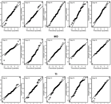
The raw residuals for the test data are defined to be the true output at a particular time point minus the posterior predictive means. Standardised residuals are obtained from the raw residuals by dividing by the posterior predictive standard deviations. Under the model assumptions, for each time point, the standardised residuals should be a sample of size 64 from
the central t-distribution with ˆδdegrees of freedom. This property can be assessed by using the
usual quantile-quantile (QQ) plot. Figure 1 shows the QQ plots for each of the five time points and each of the three methods. All three methods exhibit heavy-tailed standardised residuals, which according to Conti and O’Hagan (2010), is also common in single-output emulators.
Table 3.3 shows the average root mean square prediction error, based on the standardised residuals over the 64 runs and five time points. This value, under the model assumptions, has expected value of one (Conti and O’Hagan, 2010). The table also gives the frequentist coverage of the 95% probability intervals from the posterior predictive distribution, the relative mean
Figure 1: Quantile-quantile plots of the standardised residuals for the five different time points and for the three different methods.
−2 −1 0 1 2 −2 −1 0 1 2 Theoretical Quantiles Sample Quantiles Day=2 −2 −1 0 1 2 −3 −2 −1 0 1 2 3 Theoretical Quantiles Sample Quantiles Day=3 −2−1 0 1 2 −1.5 −0.5 0.5 1.5 LWE Theoretical Quantiles Sample Quantiles Day=4 −2 −1 0 1 2 −2 −1 0 1 2 Theoretical Quantiles Sample Quantiles Day=5 −2 −1 0 1 2 −2 −1 0 1 2 3 Theoretical Quantiles Sample Quantiles Day=6 −2 −1 0 1 2 −4 −3 −2 −1 0 1 2 Theoretical Quantiles Sample Quantiles Day=2 −2 −1 0 1 2 −2 −1 0 1 2 3 4 Theoretical Quantiles Sample Quantiles Day=3 −2−1 0 1 2 −3 −2 −1 0 1 2 3 MO Theoretical Quantiles Sample Quantiles Day=4 −2 −1 0 1 2 −3 −2 −1 0 1 2 Theoretical Quantiles Sample Quantiles Day=5 −2 −1 0 1 2 −4 −3 −2 −1 0 1 2 Theoretical Quantiles Sample Quantiles Day=6 −2 −1 0 1 2 −4 −2 0 2 4 6 Theoretical Quantiles Sample Quantiles Day=2 −2 −1 0 1 2 −4 −2 0 2 4 Theoretical Quantiles Sample Quantiles Day=3 −2 −1 0 1 2 −4 −2 0 2 4 TI Theoretical Quantiles Sample Quantiles Day=4 −2 −1 0 1 2 −3 −2 −1 0 1 2 Theoretical Quantiles Sample Quantiles Day=5 −2 −1 0 1 2 −4 −2 0 2 4 Theoretical Quantiles Sample Quantiles Day=6
Table 1: Root mean square prediction error (RMSPE), coverage and relative mean width of the 95%
probability intervals and relative mean squared error (MSE) of the three different methods.
Method RMSPE Coverage Relative Mean Relative MSE
Width (10−3) (10−6)
LWE 1.02 0.950 12.9 17.3
MO 1.12 0.925 6.81 3.89
TI 1.81 0.766 5.19 6.92
width of these intervals (relative to the true output) and the relative mean squared error of the posterior predictive mean and the true output, relative to the true output.
From Table 3.3 it is clear that the multivariate emulators (MO and LWE) perform well in this application. The RMSPE is near one and the coverage of the predictive probability intervals is close to the nominal value of 0.95. The mean width of these intervals is largest for the LWE indicating higher predictive variance under this model. Although the TI model has the lowest mean width, the RMSPE is furthest from one and there is under-coverage of the predictive probability intervals.
3.4. Sensitivity Analysis
In this section we determine the sensitivity of the number of civilian deaths to changes in the input variables using the LWE as a surrogate for the computer model. We follow the probabilistic sensitivity analysis outlined by Oakley and O’Hagan (2004) and consider each dimension of output separately. Since we are using the LWE, some of the intractable integrals
in Oakley and O’Hagan (2004) are evaluated as zero, which simplifies the necessary calculations.
Let G denote the distribution of the input variables and definexsto be a vector of values of
a subset of the input variables where x−s denotes the input variables not inxs. The posterior
mean of the effect ofxs is given by the k×1 vector
zs(xs) = E (E (f(x)|xs)|Y)−E (E (f(x))|Y), = MˆT (Rs(xs)−R), where Rs(xs) = Z X−s h(x)dG−s|s(x−s|xs), (13) R= Z X h(x)dG(x), (14)
and G−s|s(·|xs) is the conditional distribution of x−s given xs.
Since h(·) defines a 2nd order polynomial in the input variables, the jth element of h(x)
can be written h(x)j = 7 Y i=1 xaij i , for j = 1, ..., m, where P7
i=1aij ≤ 2 and aij ∈ {0,1,2}. Therefore the jth elements of Rs(xs)
and R are Rs(xs)j = Z X−s 7 Y i=1 xaij i dG−s|s(x−s|xs), (15) Rj = Z X 7 Y i=1 xaij i dG(x), (16) respectively.
A special case is when xs =xl, i.e. the lth input variable, for l = 1, ..., p, so that zl(xl) is
the posterior mean of the “main effect” of the lth input variable.
We specify a G such that xi
iid
∼U[0,1], fori = 1, ...,5, and xi
iid
∼Bernoulli(0.5), for i = 6,7.
Therefore (15) and (16) simplify to
Rs(xs)j = Y i∈S xaij i / Y i /∈S (aij + 1), Rj = 1/ 7 Y i=1 (aij + 1),
respectively, where S denotes the indices of the elements ofxs.
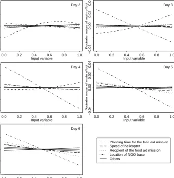
Figure 2 shows the posterior mean of the main effect of each of the input variables for each of the time points. We have only uniquely identified the planning time for the food aid
Figure 2: Posterior mean of the main effects for each of the input variables and each time point, plotted against the input variable. We have only uniquely identified planning time for the food aid mission, speed of the helicopter, and the two categorical input variables.
0.0 0.2 0.4 0.6 0.8 1.0 −0.04 0.00 0.02 0.04 Input variable P oster
ior mean of main eff
ect Day 2 0.0 0.2 0.4 0.6 0.8 1.0 −0.04 0.00 0.02 0.04 Input variable P oster
ior mean of main eff
ect Day 3 0.0 0.2 0.4 0.6 0.8 1.0 −0.04 0.00 0.02 0.04 Input variable P oster
ior mean of main eff
ect Day 4 0.0 0.2 0.4 0.6 0.8 1.0 −0.04 0.00 0.02 0.04 Input variable P oster
ior mean of main eff
ect Day 5 0.0 0.2 0.4 0.6 0.8 1.0 −0.04 0.00 0.02 0.04 Input variable P oster
ior mean of main eff
ect Day 6
Planning time for the food aid mission Speed of helicopter
Recipient of the food aid mission Location of NGO base Others
mission, the speed of the helicopter and the two categorical input variables as the output is
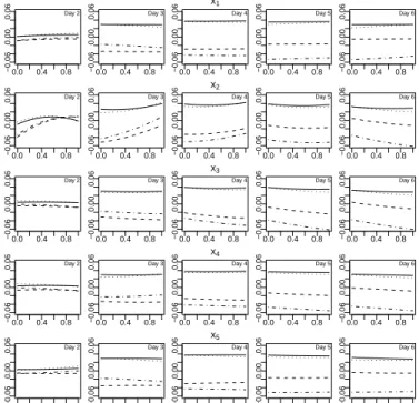
most sensitive to these four input variables. Figure 3 shows zl(xl, x6, x7) plotted against xl
for l = 1, ..., p, for each time point and for each unique combination of the categorical input
variables, x6 and x7. We can see from Figure 3 that there appears to be interaction between
the planning time for the food aid mission, x2, and the categorical input variables.
For the LWE, the most important input variables can also be determined using Bayesian model selection methods (see, for example, O’Hagan and Forster, 2004, Chapter 7). Each choice
of the function h(·), say hv(·), defines a model, v ∈ V. The posterior model probability of this
model is given by
π(v|Y)∝π(Y|v)π(v),
whereπ(Y|v) is the marginal likelihood andπ(v) is the prior model probability. In the case of
a LWE, the marginal likelihood is available in closed form as
π(Y|v) = Γ δv+n+k−1 2 πnk2 Γ δv+k−1 2 |Ωˆv| k 2 |Ωv| k 2 |Sv| δv+k−1 2 |Sˆv| δv+n+k−1 2 ,
where δv, ˆΩv, Ωv, ˆSv, and Sv are the prior and updated posterior hyperparameters associated
with model v, as defined in Section 3.2.
We assume that the function h(·) used in Section 3.3 defines the most complicated model
that we are prepared to consider. The marginality principle (McCullagh and Nelder, 1989, ch. 3) is followed so that for an interaction to be included, both linear effects must also be present in the model. Under this principle, there are approximately 72 million possible models and so even though the marginal likelihoods are available in closed form, calculating each one is
Figure 3: zl(xl) plotted against xs when x= (xs, x6, x7) for each input variable, xs, and each time point, for each unique value of the categorical input variables x6 andx7.
0.0 0.4 0.8 −0.06 0.00 0.06 Day 2 0.0 0.4 0.8 −0.06 0.00 0.06 Day 3 0.0 0.4 0.8 −0.06 0.00 0.06 x1 Day 4 0.0 0.4 0.8 −0.06 0.00 0.06 Day 5 0.0 0.4 0.8 −0.06 0.00 0.06 Day 6 0.0 0.4 0.8 −0.06 0.00 0.06 Day 2 0.0 0.4 0.8 −0.06 0.00 0.06 Day 3 0.0 0.4 0.8 −0.06 0.00 0.06 x2 Day 4 0.0 0.4 0.8 −0.06 0.00 0.06 Day 5 0.0 0.4 0.8 −0.06 0.00 0.06 Day 6 0.0 0.4 0.8 −0.06 0.00 0.06 Day 2 0.0 0.4 0.8 −0.06 0.00 0.06 Day 3 0.0 0.4 0.8 −0.06 0.00 0.06 x3 Day 4 0.0 0.4 0.8 −0.06 0.00 0.06 Day 5 0.0 0.4 0.8 −0.06 0.00 0.06 Day 6 0.0 0.4 0.8 −0.06 0.00 0.06 Day 2 0.0 0.4 0.8 −0.06 0.00 0.06 Day 3 0.0 0.4 0.8 −0.06 0.00 0.06 x4 Day 4 0.0 0.4 0.8 −0.06 0.00 0.06 Day 5 0.0 0.4 0.8 −0.06 0.00 0.06 Day 6 0.0 0.4 0.8 −0.06 0.00 0.06 Day 2 0.0 0.4 0.8 −0.06 0.00 0.06 Day 3 0.0 0.4 0.8 −0.06 0.00 0.06 x5 Day 4 0.0 0.4 0.8 −0.06 0.00 0.06 Day 5 0.0 0.4 0.8 −0.06 0.00 0.06 Day 6
infeasible. Instead we use Markov Chain Monte Carlo Model Composition (MC3, Madigan and
York, 1995). This produces a dependent sample which, if large enough, can be viewed as a
sample from v|Y.
Suppose the chain is in model v and a move to model v0 ∈ V is proposed, where v0 either
corresponds to retaining the same h(·) (i.e. v0 =v), adding a term, or removing a term, where
term refers to a linear effect of a variable or an interaction between two variables. This move
is then accepted with probability ρ= min(1, α) where
α = π(v 0|Y) π(v0|Y) = π(Y|v0)π(v0)rv π(Y|v)π(v)rv0 ,
where rv gives the number of models we can propose a move to, given that the current model
is v. If we specify that Sv =Sv0 =S and δv =δv0 =δ, for all v, v0 ∈ V, then
α= | ˆ Ωv0| k 2 |Ωv0| k 2 |Ωv| k 2 |Ωˆv| k 2 |Sˆ| δ+n+k−1 2 v |Sˆ| δ+n+k−1 2 v0 π(v0)rv π(v)rv0 .
We set S = 0 and δ = −2k, i.e. the same non-informative values we used in Section 3.3.
We also set Mv = 0. All that remains is to specify the value for Ωv which controls the prior
variance of Bv|Σv. We use the convenient g-prior of Zellner (1983),
Ω−v1 =gvHTvHv,
where gv > 0. The value of gv now controls the prior variance of Bv|Σv. It is known that
posterior model probabilities are sensitive to the prior variance of the model parameters not
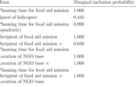
Table 2: Marginal inclusion probabilities for the possible terms inh(·) under the LWE.
Term Marginal inclusion probability
Planning time for food aid mission 1.000
Speed of helicopter 0.445
Planning time for food aid mission 0.998
(quadratic)
Recipient of food aid mission 1.000
Recipient of food aid mission × 0.650
Planning time for food aid mission
Location of NGO base 1.000
Location of NGO base × 1.000
Planning time for food aid mission
Recipient of food aid mission × 1.000
Location of NGO base
O’Hagan and Forster, 2004, pp 77-78), the posterior model probability of the simplest model,
i.e. h(x) = 1, will tend to one.
We set gj = g = n−1 which results in the unit-information prior proposed by Kass and
Wasserman (1995) for linear models. It amounts to the prior distribution for Bv|Σv providing
the same amount of information as one run of the computer model. Non-informative prior
model probabilities are specified asπ(v)∝1.
We run the MC3 algorithm for 2.5×10⁴ iterations, after a burn-in phase of 104 iterations
and starting at the most complicated model. The marginal inclusion probability of a term is
defined to be the posterior probability of including that particular term inh(·), estimated using
the MC3 sample from v|Y as the proportion of models in the chain that include that term.
Table 3.4 shows marginal inclusion probabilities greater than 0.05 for the 33 possible terms. These probabilities support the conclusions from the traditional sensitivity analysis above, i.e. the input is sensitive to the planning time for the food aid mission, the speed of the helicopter and the two categorical input variables.
3.5. Discussion of example 1
From Section 3.3, it appears that the MO method outperforms the TI method in terms of predictive ability in this application. Conti and O’Hagan (2010) came to the same
conclu-sion when they compared the two methods on an example where k = 60 and there were ten
continuous input variables.
In addition to the Gaussian process models, we applied the LWE. Although this model was inferior to the MO model in terms of predictive ability, it can be fitted in fractions of a second
as we do not need to find a value to use for ˆr.
In Section 3.4 we use the LWE as a surrogate for the computer model. In the traditional probabilistic sensitivity analysis, many of the integrals in Oakley and O’Hagan (2004) are zero, simplifying the approach significantly. We also used Bayesian model determination to identify the most important input variables. Both approaches concluded that the output was most
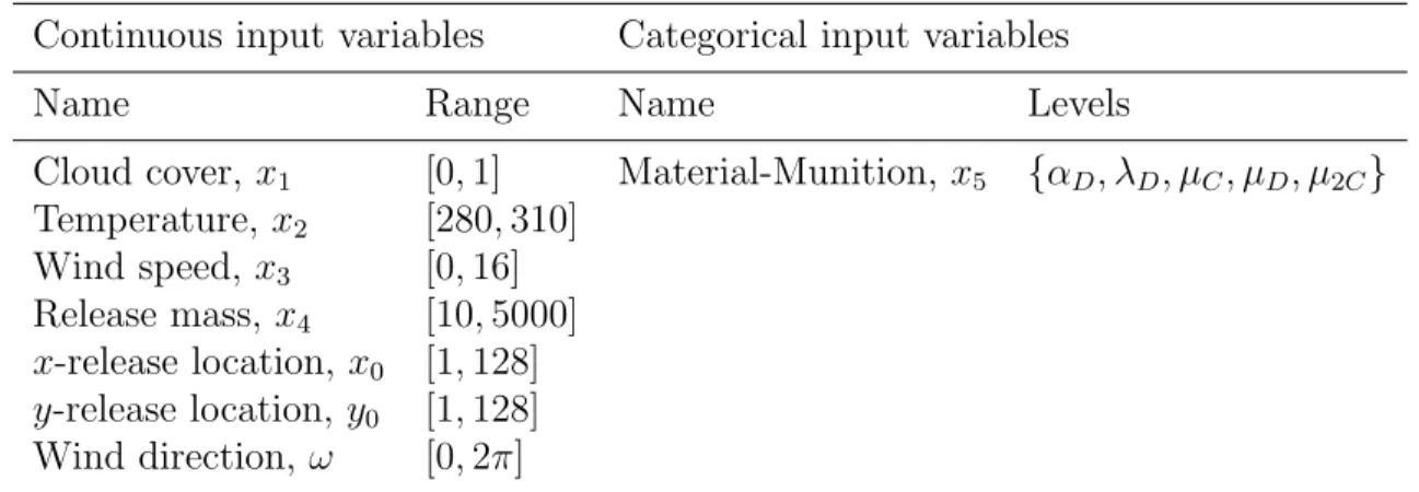
Table 3: Input variables for the dispersion model.
Continuous input variables Categorical input variables
Name Range Name Levels
Cloud cover, x1 [0,1] Material-Munition, x5 {αD, λD, µC, µD, µ2C}
Temperature, x2 [280,310] Wind speed,x3 [0,16] Release mass, x4 [10,5000] x-release location, x0 [1,128] y-release location, y0 [1,128] Wind direction, ω [0,2π]
sensitive to the planning time for the food aid mission, the speed of the helicopter, and the two categorical input variables. There is also strong evidence of interactions between the planning time for the food aid mission and the categorical inputs.
With the LWE a further approach would be to undertake the Bayesian model determination to obtain the posterior model probabilities. We could then use Bayesian model averaging to find the posterior predictive distribution, i.e. the emulator. The emulator would then be a mixture of multivariate t-distributions where the weights are given by the posterior model probabilities. However we would then lose the “light weightness” of the LWE over the Gaussian process.
4. A dispersion model: a computer model with multivariate zero-inflated output 4.1. Introduction
The simulator considered in this section is called a dispersion model. It models the dispersion of particles, over a given terrain, after a chemical or biological particles release. Here, the terrain
is represented as a 128×128 grid.
Let Yi = f(xi) denote the k ×1 vector of output of the computer model given the input
variablesxi, wherek = 1282 = 16384. Each element,Yij, of Yi forj = 1, ..., k, gives the dosage
observed at a particular location, indexed byj, on the grid. Table 4.1 shows the input variables
for this computer model which are both continuous and categorical. Let Y = YT 1 .. . Yn ,
be the n×k matrix of outputs.
There are two challenges to overcome when emulating this computer model. The first is the
high dimensionality, k, of the output. The second is that the output is zero-inflated.
Regarding the high dimensionality, Woods and Lewis (2009) emulated this computer model using the approach of Higdon et al. (2008). Consider the singular value decomposition (SVD)
Figure 4: Plumes for two runs of the computer model.
Run= 44 Run= 448
where U is a k ×n orthogonal matrix, D is an n×n diagonal matrix of the singular values
and V is an n×n orthonormal matrix. Aq-dimensional principal component basis,b1, ...,bq,
is given by the first q ≤ n columns of n−12UD with weights, wj(xi), given by the jith entry
of n12VT. We relate the q n×1 vectors, w1, ...,wq, where wj = (wj(x1), ..., wj(xn)), using q
Gaussian process models. We then predict y0 =f(x0) using
y0 =
q X
j=1
bqwˆj(x0),
where ˆwj(x0) is the prediction of the jth Gaussian process at x0. For more details on this
approach see Woods and Lewis (2009). However, in this section we instead use a lightweight emulator.
4.2. Methodology
4.2.1. Emulator We have output from 474 runs of the simulator with which to construct and test the emulator. These runs are historical data rather than a designed experiment.
Figure 4 shows the output from two runs, 44 and 448, of the computer model. Black signifies that no dosage was observed at that location and white signifies that a high dosage was observed. The shapes in Figure 4 are called plumes.
It is not feasible to use the LWE described in Section 3.2 wherek = 16384. Also this method
is not appropriate for zero-inflated output.
To reduce the dimensionality we consider the output to be scalar, with the location where the dosage is observed as extra input variables. This is a generalisation of the time-input
Gaussian process, considered in Section 3.2, to spatial inputs. Associated with each Yij is
the location variables, (Xij,Yij), where Yij was observed, with 1 ≤ Xij,Yij ≤ 128. Note that
Xij =Xlj and Yij =Ylj, for all l, i = 1, ..., N and j = 1, ..., k.
We transform the location variables for the ith run, equivalent to rotating and shifting the
grid so that the release is always at the origin and the wind direction is always π. We also
rij2 = (Xij −x0i)2 + (Yij −y0i)2, (17) θij = arctanYij−y0i Xij−x0i +π−ω if ω ≥0, arctanYij−y0i Xij−x0i −π−ω if ω < 0. (18)
Now associated with eachYij is thep×1 vector of input variablesx∗ij = (x1i, x2i, x3i, x4i, x5i, rij, θij)
wherep= 7. Note that wind direction and release location are now constant for all (i, j) so no
longer feature in the vector of input variables. Studying dispersion where the release location and the wind direction are constant follows from Clarke (1979), albeit in Cartesian co-ordinates as opposed to polar.
We use the odd-numbered runs to build the emulator and the even-numbered runs to test.
Therefore n = 237. The vector of output now has nk ≈ 3.9 million elements. This will be
too large for sensible computation. We make the assumption that if the location is upwind of the release, then the observed dosage will be zero. Therefore we remove all observations
such that θij ∈/ −π 2, π 2
. This leaves approximately 2.7 million observations. We subsample,
without replacment, ni observations within each run of the computer model so that we have
n∗ =Pni=1ni observations, labelled Y∗.
We therefore have n∗ output values which are zero-inflated. A standard statistical model
for analysing zero-inflated continuous responses is the Tobit regression model (Tobin, 1958). Chib (1992) considered Bayesian inference for the Tobit model deriving a method to obtain a sample from the posterior distribution of the model parameters using Gibbs sampling.
We assume that the latent variables, Zi, have independent normal distributions
Zi ∼N h(xi)Tβ, σ2
,
for i = 1, ..., n∗ and we osberve Yi∗ = max(Zi,0). We specify the following conditionally conjugate prior distributions:
β|σ2 ∼ N m, σ2Ω, σ2 ∼ IG δ 2, s 2 .
Let C = {i:Yi∗ = 0, i= 1, ..., n∗} identify the output values that are identically zero. The Gibbs sampling scheme for the Tobit model is:
1. Let the current model parameters be β(j) and σ2(j).
2. For i ∈ C, generate a latent variable Zi(j+1) from N
h(x∗i)Tβ(j), σ2(j) , truncated to (−∞,0). Let Ri = Yi∗ if i /∈C, Zi(j+1) if i∈C, and R= (R1, ..., Rn∗)T.
3. Let ˆ Ω = HTH+Ω−1−1 , ˆ m = Ω Hˆ TR+Ω−1m, ˆ δ = δ+n∗, ˆ s = s+RTR+mTΩ−1m−mˆTΩˆ−1mˆ. 4. Generate σ2(j+1) from IGˆδ 2, ˆ s 2 . 5. Generate β(j+1) from Nmˆ, σ2(j+1)Ωˆ.
Although the posterior distributions are not available in closed form, the above algorithm is still computationally inexpensive since the full conditional distributions are known, so therefore we do not need to use any rejection sampling methods.
We now have a sample, n
β(1), σ2(1), ...,β(B), σ2(B)o ,
from the posterior distribution of β and σ2. To evaluate the posterior predictive distribution,
y0|Y∗, where y0 = f(x0), let y0j be the jth element of y0, for j = 1, ..., k. We can find a
posterior sample from y0j|Y∗ by generating
z0(tj)∼Nh(x0∗j)Tβ(t), σ2(t),
where x∗0j = (x10, x20, x30, x40, x50, r0j, θ0j), and then setting y
(t)
0j = max(0, z
(t)
0j), fort = 1, ..., B.
This is the fully Bayesian approach. The alternative plug-in approach is less computationally
expensive and is the approach taken in this paper. Let ˆβ and ˆσ2 be representative values ofβ
and σ2, respectively, relative to β, σ2|Y∗. The plug-in approach is that y
0j|Y∗ is the censored
normal distribution, formed by taking y0j = max (0, z0j), with
z0j ∼N
h(x∗0j)Tβ,ˆ σˆ2 .
4.3. Results
Let ni = 50, for i = 1, ...,237, resulting in n∗ = 11850. Only 30% of the sampled Yi∗s are
non zero, indicating the high level of zero-inflation.
After taking logarithms of wind speed, x3 and release mass, x4, we specify an h(·) that
corresponds to an intercept, all linear effects, all two-way interactions and quadratic terms
for the continuous input variables; thus m = 56. We use non-informative choices for the
hyperparmeters of the prior of β and σ2, i.e. m=0, Ω−1 =0, s= 0 and δ=−2.
A sample of size B = 104 is generated from β, σ2|Y∗ using the Gibbs sampling scheme,
after a burn-in phase of 5×10³ iterations. We set ˆβ and ˆσ2 to be the sample means of β and
σ2, respectively.
We use the test runs of the computer model to evaluate the emulator. We find the posterior mean of each location of each test run and also the 95% posterior predictive probability interval
Figure 5: Predicted plumes for two runs of the computer model. 0.0 0.2 0.4 0.6 0.8 1.0 0.0 0.2 0.4 0.6 0.8 1.0 x−location y−location 0.0 0.2 0.4 0.6 0.8 1.0 0.0 0.2 0.4 0.6 0.8 1.0 x−location y−location 0.0 0.2 0.4 0.6 0.8 1.0 0.0 0.2 0.4 0.6 0.8 1.0 x−location y−location 0.0 0.2 0.4 0.6 0.8 1.0 0.0 0.2 0.4 0.6 0.8 1.0 x−location y−location
by taking the 2.5th and 97.5th quantiles of the posterior predictive distribution as the lower
and upper limits, respectively. Explicitly the rth quantile is given by
y0(rj) = 0 if r < Φ −h(x ∗ 0j)Tβˆ ˆ σ , h(x∗0j)Tβˆ+ Φ−1(r)ˆσ otherwise. where x∗0j = (x10, x20, x30, x40, x50, r0j, θ0j).
The coverage of the intervals is 0.998 with a mean width of 2.07×10⁻⁴. The MSE between
the predictive mean and the true dosage is 3.84×10⁻³. The value of MSE is of the same order
as the MSE obtained by Woods and Lewis (2009) for the same computer model but using a Gaussian process as the emulator as described in Section 4.1.
Figure 5 shows the true plumes for runs 44 and 448 (featured in Figure 4) and the corre-sponding plume where we have used the posterior predictive mean as the point prediction.
4.4. Sensitivity Analysis
In this section we conduct a sensitivity analysis to identify the most important input vari-ables. This sensitivity analysis is undertaken under a fixed wind direction and release location. To incorporate an unknown wind direction or release location we would just transform the
locations, r and θ, using the inverse of the transformation given by (17) and (18).
The mean of the posterior predictive distribution of the dosage at the location given by r
and θ, given the input variablesx1, ..., x5 is
µ(x1, ..., x5;r, θ) = ˆη 1−Φ −ηˆ ˆ σ + ˆσφ −ηˆ ˆ σ , (19) where ˆη=h(x∗)Tβˆ and x∗ = (x 1, ..., x5, r, θ).
The posterior mean of the main effect of the lth input variable,xl, at the location given by r and θ, is zl(xl;r, θ) = Rl(xl;r, θ)−R(r, θ), where Rl(xl;r, θ) = Z X−l µ(x1, ..., x5;r, θ)dG−l|l(x−l|xl), (20) R(r, θ) = Z X µ(x1, ..., x5;r, θ)dG(x), (21)
for l = 1, ...,5, where G denotes the joint distribution of the input variables x1, ..., x5. The
integrals involved in (20) and (21) will be analytically intractable for a typical G so we use
Monte Carlo methods to approximate these quantities. To approximate Rl(xl;r, θ), we
gen-erate x(−i)l from G−l|l and evaluate µ(x1, ..., x5;r, θ)(i) using (19), for i = 1, ..., B. We then
approximateRl(xl;r, θ) as the mean of the µ(x1, ..., x5;r, θ)(i)s. It is straightforward to extend
this methodology to approximate R(r, θ).
For G, we let xl
iid
∼ U [0,1], for l = 1, ...,4 and let x5 be discretely uniform on the set
{αD, λD, µC, µD, µ2C}.
We investigate the sensitivity of the dosage to changes in the input variables at six different locations, also shown in Figure 6:
1. (r, θ) = (0.10,0), 2. (r, θ) = (0.25,0), 3. (r, θ) = (0.50,0), 4. (r, θ) = (0.10, π/8), 5. (r, θ) = (0.25, π/8), 6. (r, θ) = (0.50, π/8).
The first three locations lie on the up-downwind axis in the downwind direction at three different distances from the release. The second three locations are further away from the up-downwind axis.
Figure 7 shows zl(xl;r, θ) plotted againstxl, for the six locations shown in Figure 6 and for
l = 1,2,3,4, i.e. the continuous input variables. Also shown in Figure 7, as grey horizontal
lines, are the values of z5(x5;r, θ) for the five different levels of the material-munition input
variable.
The predicted dosage is most sensitive to changes in release mass and wind speed when
the location is close to the release location, i.e. when r = 0.1. As r increases, i.e. the
location becomes further from the release location, the predicted dosage becomes less sensitive to changes in all of the input variables. This indicates that there are interactions between the
input variables and r.
When r = 0.1, increasing the release mass increases the predicted dosage, whilst increasing
the wind speed decreases the predicted dosage. This is in agreement with the simple Gaussian plume model of Clarke (1979).
Figure 6: The six locations where we investigate the dosage sensitivity to the input variables. −1.0 −0.5 0.0 0.5 1.0 −1.0 −0.5 0.0 0.5 1.0 x y 41 2 3 5 6
Figure 7: Plot ofzl(xl;Xnew,Ynew) againstxl at the six locations shown in Figure 6.
0.0 0.2 0.4 0.6 0.8 1.0 −0.003 −0.001 0.001 0.003 Input variable P oster
ior mean of main eff
ect (r,θ)=(0.1,0) 0.0 0.2 0.4 0.6 0.8 1.0 −0.003 −0.001 0.001 0.003 Input variable P oster
ior mean of main eff
ect (r,θ)=(0.1,π/8) 0.0 0.2 0.4 0.6 0.8 1.0 −0.003 −0.001 0.001 0.003 Input variable P oster
ior mean of main eff
ect (r,θ)=(0.25,0) 0.0 0.2 0.4 0.6 0.8 1.0 −0.003 −0.001 0.001 0.003 Input variable P oster
ior mean of main eff
ect (r,θ)=(0.25,π/8) 0.0 0.2 0.4 0.6 0.8 1.0 −0.003 −0.001 0.001 0.003 Input variable P oster
ior mean of main eff
ect (r,θ)=(0.5,0) 0.0 0.2 0.4 0.6 0.8 1.0 −0.003 −0.001 0.001 0.003 Input variable P oster
ior mean of main eff
ect (r,θ)=(0.5,π/8)
We can also determine the most important input variables using Bayesian model selection. The marginal likelihoods, and therefore the posterior model probabilities, of Tobit models are not available analytically. Gawande (1998) proposed a Monte Carlo method for approximation of the marginal likelihood using the marginal likelihood identity method of Chib (1995). How-ever there are approximately 143 million possible models rendering this approach infeasible. Instead we introduce a model update step into the Gibbs sampling scheme in Section 4.2.
Let each possible Tobit model be indexed by v ∈ V where V is the set of possible models.
The model selection Gibbs sampling scheme is:
1. Let the current model parameters be β(vj()j),σ
2(j)
v(j) and v
(j).
2. For i ∈ C, generate a latent variable Zi(j+1) from Nhv(j)(x∗i)Tβ
(j) v(j), σ 2(j) v(j) truncated to (−∞,0). Let Ri = Yi∗ if i /∈C, Zi(j+1) if i∈C, and R= (R1, ..., Rn∗)T.
3. Propose a new model v0 and accept this move with probability min(1, a) where
a= | ˆ Ωv0| 1 2 |Ωv0| 1 2 |Ωv(j)| 1 2 |Ωˆv(j)| 1 2 ˆ sv(j) ˆ sv0 π(v0) π(v(j)) rv(j) rv0 .
If the move is accepted, then v(j+1) =v0, otherwisev(j+1) =v(j).
4. Generate σv2((jj+1)+1) from IG ˆ δv(j+1) 2 , ˆ sv(j+1) 2 . 5. Generate β(vj(+1)j+1) from N ˆ vv(j+1), σ 2(j+1) v(j+1)Ωˆv(j+1) .
We are certain that r and θ and their interaction are terms in h(·), so we set π(v) = 0 for
all models with anhv(·) that does not contain these three terms. The prior over the remaining
models is uniform. Explicitly
π(v)∝
0 if hv(·) does not containr, θ or their interaction,
1 otherwise.
For the prior distributions for the model parameters, we set Ω−v1 = n1∗HTvHv, sv = 0, δv = 0
and mv =0.
We run the above model selection Gibbs sampling scheme for a total of 2.5×10⁴ iterations
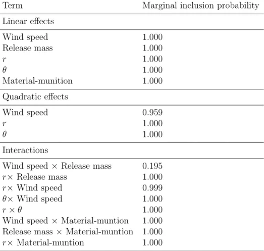
after a burn-in phase of 104 iterations. Table 4.4 shows the marginal inclusion probabilities
greater than 0.1. The terms included in Table 4.4 agree with our conclusions from the traditional sensitivity analysis, i.e. that the predicted dosage is most sensitive to changes in wind speed and release mass, and that there exist interactions between the input variables and the distance
Table 4: Marginal inclusion probabilities for possible terms in h(·).
Term Marginal inclusion probability
Linear effects Wind speed 1.000 Release mass 1.000 r 1.000 θ 1.000 Material-munition 1.000 Quadratic effects Wind speed 0.959 r 1.000 θ 1.000 Interactions
Wind speed× Release mass 0.195
r× Release mass 1.000
r× Wind speed 0.999
θ× Wind speed 1.000
r×θ 1.000
Wind speed× Material-muntion 1.000
Release mass ×Material-muntion 1.000
4.5. Discussion of example 2
In this section we used a generalisation of the LWE to zero-inflated output. The posterior distributions were not available in closed form but a computationally cheap Gibbs sampling algorithm was used to generate a sample from these distributions.
We carried out a sensitivity analysis, in the traditional sense and via Bayesian model se-lection, and found that the dosage was most sensitive to changes in the release mass and wind speed, and the relationships change as the location moves away from the release location.
Currently, the accuracy of the emulator is suitable for qualitative predictions, and as such is useful for identifying key trends and input variables with substantive impact and also informing broad policy decisions in, for example, military planning and emergency response.
5. Conclusions
In this article, we used lightweight emulation in two challenging computer model applica-tions. The key feature of lightweight emulation is to model the features of the computer model through the mean function as opposed to the covariance structure, as in a Gaussian process.
In the first application, the humanitarian relief mission computer model, the lightweight emulator had predictive accuracy only an order of magnitude less than that of the standard Gaussian process, but allowed us to undertake an analytic sensitivity analysis and a Bayesian model comparison to identify the most important input variables.
In the second application, the dispersion computer model, the lightweight emulator did not have entirely satisfactory predictive accuracy but, nevertheless, a descriptive model was produce that allowed us to undertake a useful sensitivity analysis to identify important input variables.
The lightweight emulator has great scope for generalisation. For instance, suppose the output of the computer model was distinctly non-normal, then a class of models which could be used as a lightweight emulator are generalised linear models (GLMs).
6. Acknowledgments
This work was funded by a Defence Threat Reduction Agency basic research grant and the Defence Science and Technology Laboratory (Dstl). The authors wish to thank Dr Veronica Bowman and Robin Ashmore from Dstl for providing the simulators and data for the two examples, and related invaluable conversations.
7. References
1. Berger, J., De Oliveira, V., and Sanso, B. (2001). Objective Bayesian analysis of spatially
correlated data. Journal of the American Statistical Association, 96, 1361-1374.
2. Chib, S. (1992). Bayes inference in the Tobit censored regression model. Journal of
Econometrics, 51, 79-99.
3. Chib, S. (1995). Marginal Likelihood from the Gibbs Output. Journal of the American
Statistical Association, 90, 1313-1321.
a Model for Short and Medium Range Dispersion of Radionuclides Released to the Atmo-sphere. London: Her Majesty’s Stationary Office.
5. Conti, S. and O’Hagan, A. (2010). Bayesian Emulation of Complex Multi-Output and
Dynamic Computer Models. Journal of Statistical Planning and Inference,140, 640-651.
Dawid, A.P. (1981). Some matrix-variate distribution theory: Notational considerations
and a Bayesian application. Biometrika, 68, 265-274.
6. Fang, K., Li, R. and Sudjianto, A. (2006). Design and Modeling for Computer
Experi-ments. Chapman and Hall.
7. Gawande, K. (1998). Comparing Theories of Endogenous Protection: Bayesian
Com-parison of Tobit Models using Gibbs Sampling Output. The Review of Economics and
Statistics, 80, 128-140.
8. Higdon, D., Gattiker, J., Williams, B. and Rightley, M. (2008). Computer Model
Calibra-tion Using High-Dimensional Output. Journal of the American Statistical Association,
103, 570-583.
9. Kennedy, M.C. and O’Hagan, A. (2001). Bayesian calibration of computer models (with
discussion). Journal of the Royal Statistical Society, B, 63, 425-464.
10. Kotz, S. and Nadarajah, S. (2004). Multivariate t Distributions and Their Applications.
Cambridge.
11. Madigan, D. and York, J. (1995). Bayesian graphical models for discrete data.
Interna-tional Statistics Review,63, 215-232.
12. McCullagh, P. and Nelder, J. (1989). Generalised Linear Models (2nd ed.). Chapman
and Hall.
13. McKay, M.D., Conover, W.J. and Beckman, R.J. (1979). A Comparison of Three Methods for Selecting Values of Input Variables in the Analysis of Output from a Computer Code.
Technometrics, 21, 239-245.
14. Morris, M.D. and Mitchell, T.J. (1995). Exploratory Designs for Computer Experiments.
Journal of Statistical Planning and Inference,43, 381-402.
15. Oakley J.E. and O’Hagan, A. (2004). Probabilistic Sensitivity Analysis of Complex
Mod-els: A Bayesian Approach. Journal of the Royal Statistical Society, B, 66, 751-769.
16. O’Hagan, A. and Forster, J.J. (2004). Kendall’s Advanced Theory of Statistics, Volume
2B: Bayesian Inference. (2nd edition). Arnold.
17. Qian, P.Z., Wu, H. and Wu, C.F.J. (2008). Gaussian Process Models for Computer
Experiments with Qualitative and Quantitative Factors. Technometrics, 50, 383-396.
18. Qian, P.Z. and Wu, C.F.J. (2009). Sliced space-filling designs. Biometrika,96, 945-956.
19. Rougier, J. (2007). Lightweight emulators for Multivariate Deterministic Functions.
20. Rougier, J. (2008). Efficient emulators for multivariate deterministic functions. Journal of Computational and Graphical Statistics, 17, 827-843.
21. Sacks, J., Welch, W.J., Mitchell, T.J. and Wynn, H.P. (1989). Design and analysis of
computer experiments. Statistical Science,4, 409-435.
22. Saltelli, A., Chan, K. and Scott, M. (2000). Sensitivity Analysis. Wiley.
23. Santner, T.J., Williams, B.J. and Notz, W.I. (2003). The Design and Analysis of
Com-puter Experiments. Springer.
24. Tobin, J. (1958). Estimation of relationships for limited dependent variables.
Economet-rica, 26, 24-36.
25. Woods, D.C. and Lewis, S.M. (2009). Surrogate-modelling for computer experiments with multi-dimensional responses. Technical Report, Southampton Statistical Sciences Research Institute, University of Southampton, United Kingdom.
26. Zellner, A. (1983). Applications of Bayesian Analysis in Econometrics. Journal of the