fifteen methods
Laurent Albera, Amar Kachenoura, Pierre Comon, Ahmad Karfoul, Fabrice
Wendling, Lotfi Senhadji, Isabelle Merlet
To cite this version:
Laurent Albera, Amar Kachenoura, Pierre Comon, Ahmad Karfoul, Fabrice Wendling, et al.. ICA-based EEG denoising: a comparative analysis of fifteen methods. Bulletin of the Polish Academy of Sciences - Technical sciences, Polish Academy of Sciences, 2012, 60 (3 Special issue on Data Mining in Bioengineering), pp.407-418. <10.2478/v10175-012-0052-3>. < hal-00740304>
HAL Id: hal-00740304
https://hal.archives-ouvertes.fr/hal-00740304
Submitted on 9 Oct 2012
HAL is a multi-disciplinary open access
archive for the deposit and dissemination of sci-entific research documents, whether they are
pub-lished or not. The documents may come from
teaching and research institutions in France or abroad, or from public or private research centers.
L’archive ouverte pluridisciplinaire HAL, est
destin´ee au d´epˆot et `a la diffusion de documents
scientifiques de niveau recherche, publi´es ou non,
´emanant des ´etablissements d’enseignement et de
recherche fran¸cais ou ´etrangers, des laboratoires
ICA-based EEG denoising: a comparative
analysis of fifteen methods
Laurent Albera
(1,2), Amar Kachenoura
(1,2), Pierre Comon
(3),
Ahmad Karfoul
(4), Fabrice Wendling
(1,2), Lotfi Senhadji
(1,2),
Isabelle Merlet
(1,2)(1)INSERM, UMR 1099, F-35000 Rennes, France (2)Université de Rennes 1, LTSI, F-35000 Rennes, France
(3)CNRS, UMR5216, GIPSA-Lab, BP.46, F-38402 St Martin d’Heres cedex, France (4)Al-Baath University, Faculty of Mechanical and Electrical Engineering, PB. 2244, Homs,
Syria
For correspondence: Pierre Comon
E-Mail: [email protected]
Abstract
Independent Component Analysis (ICA) plays an important role in biomedical engineering. Indeed, the complexity of processes involved in biomedicine and the lack of reference signals make this blind approach a powerful tool to extract sources of interest. However, in practice, only few ICA algorithms such as SOBI, (extended) InfoMax and FastICA are used nowadays to process biomedical signals. In this paper we raise the question whether other ICA methods could be better suited in terms of performance and computational complexity. We focus on ElectroEncephaloGraphy (EEG) data denoising, and more particularly on removal of muscle artifacts from interictal epileptiform activity. Assumptions required by ICA are discussed in such a context. Then fifteen ICA algorithms, namely JADE, CoM2, SOBI, SOBIrob,
(extended) InfoMax, PICA, two different implementations of FastICA, ERICA, SIMBEC, FOBIUMJAD,
TFBSS, ICAR3, FOOBI1 and 4-CANDHAPc are briefly described. Next they are studied in terms of
performance and numerical complexity. Quantitative results are obtained on simulated epileptic data generated with a physiologically-plausible model. These results are also illustrated on real epileptic recordings.
I. INTRODUCTION
The removal of muscular artifacts from ElectroEncephaloGraphic (EEG) data is a crucial preprocessing step for further analysis of EEG in the diagnosis of epilepsy from Video-EEG recordings. Indeed, in the particular context of epilepsy, EEG signals of interest, such as interictal spikes or ictal discharges, may be corrupted by muscular or myogenic activity arising from the contraction of head muscles. As already reported [45], these artifacts are difficult to remove. This is especially due to i) their high amplitude (possibly several times larger than the EEG signal), ii) the large frequency range of their components and iii) their variable topographical distribution. Due to the complexity of the involved physiological processes and the lack of reference signals, researchers have mostly considered Blind Source Separation (BSS) techniques to solve the EEG denoising problem [29], [30], [42], [51], [52].
Among BSS approaches, Independent Component Analysis (ICA) is one of the most famous, especially in biomedical engineering [1], [21]. It was historically the first to be applied to EEG denoising for muscular activity [45], [47], [53]. Indeed, by assuming that EEG data can be modeled as a noisy static mixture of mutual independent sources associated with different physiological phenomena, ICA is generally considered as a powerful tool for extracting the EEG signals of interest [31], [32], [48]. However to date, only a few ICA algorithms such as SOBI [5], [58], (extended) InfoMax [39], [43] and FastICA [14, ch.6] are used in practice to process biomedical signals.
In this paper, we have examined whether other ICA methods perform better or enjoy lower computational complexity, especially for the removal of muscle artifacts from interictal epilep-tiform activity. We first discuss the EEG denoising problem and the assumptions required by ICA. Second, classical statistical tools are provided in order to understand how the ICA concept can be implemented. Next, representative methods of two classes, including the most used ICA techniques in signal processing, are briefly described and studied in terms of performance and numerical complexity: techniques based on the Differential Entropy (DE) such as (extended) InfoMax [39], [43], PICA [35] and two different implementations of FastICA [14, ch.6] versus cumulant-based methods. Among cumulant-based techniques, representative algorithms of three subfamilies are studied: i) the techniques using only SO statistics of the data such as SOBI [5], [58], SOBIrob [6], TFBSS [24], ii) the algorithms based on SO and FO statistics such as
JADE [9], CoM2 [13], and iii) the methods requiring only HO statistics such as ERICA [19],
SIMBEC [20], FOBIUMJAD [22], [23], ICAR3 [2], [3], FOOBI1 [38], 4-CANDHAPc [33], [34].
Quantitative results are obtained on simulated epileptic data generated with a physiologically-plausible model [16]–[18]. These results are also illustrated on real data recorded in a patient with epilepsy.
II. PROBLEM FORMULATION AND ASSUMPTIONS
Let’s model the EEG signal recorded fromN electrodes as one realization of anN-dimensional random vector process {x[k]}. Each random vector x[k] can then be written as the following noisy static mixture of statistical random processes called sources:
x[k] =A(e)s(e)[k] +A(b)s(b)[k] +A(m)s(m)[k] +n[k]
x[k] =A s[k] +n[k] (1)
where {s(e)[k]}, {s(b)[k]}, {s(m)[k]}, {n[k]} are random vector processes representing the P
e epileptic activity sources, the Pb background activity sources, the Pm muscular activity sources and the N-dimensional instrument noise, respectively. The mixing matricesA(e), A(b) and A(m)
model the transfer from all possible sources of activity within the brain to scalp electrodes. The assumption of static linear model comes from the mathematical formulation of the EEG/MEG forward problem. More precisely it comes from the use of the quasi-static formulation of Maxwell’s equations, called Poisson’s equations, in order to compute the electrical transfer between the cortex and the scalp [50]. Indeed, the time-derivatives of the associated electric fields are sufficiently small to be ignored in classical Maxwell’s equations. As far as the statistical properties of vector random process {s(e)[k]}, {s(b)[k]}, {s(m)[k]} and {n[k]} are concerned,
we can assume that they are independent as they correspond to different physiological/physical phenomena. Nevertheless, such an assumption is not valid within each vector random processes regarding its components. In particular, the Pe epileptic activity sources of {s(e)[k]} may be statistically mutually dependent. Eventually, the {n[k]} vector random process can be assumed to be Gaussian as most of instrument noises.
Consequently, by using ICA, at best we can hope to identify three vector subspaces corre-sponding to the epileptic sources, the muscular sources and the background sources, respectively, but not exactly the Pe +Pb +Pm sources involved in equation (1). Note that this subspace
identification is sufficient for the EEG denoising problem since we don’t want to exactly extract the Pe epileptic sources; in fact, we just want to remove the contribution of the muscular and background activities from the scalp data. Indeed, once the epileptic source subspace is identified by applying ICA to the scalp data, we get an estimate of A(e)s(e)[k] for every time index m,
say an estimate of the denoised scalp data. Nevertheless, as shown in section V, the estimation of the three subspace dimensions remains a difficult issue.
III. STATISTICAL TOOLS AND ICAMETHODS
A. Statistical tools characterizing mutual independence
Let’s recall how to characterize the statistical independence of a set of P random signals
{yp[k]}m∈N and how to use it in order to blindly separate mixed mutually independent sources. A random vector y = [y1,· · ·, yP]T has mutually independent components if and only if its Probability Density Function (PDF) py can be decomposed as the product of the P marginal PDFs, pyp, where pyp denotes the PDF of the p-th component yp of y.
Then a natural way of checking whether y has independent components is to measure a pseudo-distance between py and
Q
ppyp. Such a measure can be chosen among the large class of f-divergences. If the Kullback divergence is used, we get the Mutual Information (MI) of y
[14]: MI(y) = Z RP py(u) log py(u) QP p=1pyp(up) ! du (2)
It can be shown that the MI vanishes if and only if the P components of y are mutually independent, and MI is strictly positive otherwise.
Another measure based on the PDF of y is the DE of y:
S(y) =−
Z
RP
py(u) log(py(u))du=−E[log(py(y))] (3) sometimes referred to as Shannon’s joint entropy, where E[·]denotes the mathematical expecta-tion. This entropy is not invariant by an invertible change of coordinates, but only by orthogonal transforms. A fundamental result in information theory is that the DE can be used as a measure of non-gaussianity. Indeed, among the random vectors having an invertible covariance matrix, the Gaussian vector is the one that has the largest entropy. Then, to obtain a measure of non-gaussianity of y that is i) zero only for a Gaussian vector, ii) always positive and iii) invariant
by any linear invertible transformation, one often uses a normalized version of the DE, called
negentropy, and given by [14, ch.3]:
J(y) = S(z)−S(y) (4)
where z stands for the Gaussian vector with the same mean and covariance matrix as y. Since MI and negentropy are simply related to each other [13], estimating the negentropy allows to estimate the MI. However, even if consistent estimators of PDFs exist (e.g. Parzen estimators [55]), the computation of integral (3) is time consuming, and often prohibitive.
A way to avoid the exact computation of the negentropy consists in using another measure of statistical independence that is less accurate but easier to compute. The contrast function [13, definition 5] built from the data cumulants satisfies this condition. From now on, we shall assume that all random variables are real. If we consider Φx(u) =E[exp(iuTx)] as the first characteristic function of a random vector x, since Φx(0) = 1 and Φx is continuous, then there exists an open neighborhood of the origin, in which Ψx(u) = log(Φx(u)) can be defined. The r-th order moments are the coefficients of the Taylor expansion of Φx about the origin, up to a multiplicative coefficient ir/r!. Similarly cumulants, denoted by C
i,j,···,`,x, are the coefficients of the second characteristic function, Ψx, up to a multiplicative coefficient of the same form [14, ch.3]. It is noteworthy that the components of the (N×N) well-known covariance matrix
of an N-dimensional random vector x exactly match the Second Order (SO) cumulants of x. By analogy, the (N2×N2) matrix containing the Fourth Order (FO) cumulants of x is usually
called the quadricovariance matrix.
Cumulants are more appropriate than moments for ICA context. Indeed, cumulants enjoy two important properties. First, if at least two components or groups of components of x are statistically independent, then all cumulants involving these components are null. For instance, if all components of x are mutually independent, then Ci,j,···,`,x =δ[i, j,· · ·, `]Ci,i,···,i,x, where the Kronecker δ[i, j,· · ·, `]equals 1when all its arguments are equal and is null otherwise. Second, if x is Gaussian, then all its Higher Order (HO) cumulants, i.e. cumulants of order strictly greater than two are null. So HO cumulants may be seen as a distance to normality. Note that moments do not enjoy these two key properties. Moments and cumulants share two other useful properties. On the one hand, they are both symmetric arrays, since the value of their entries does not change by permutation of their indices. Consequently, covariance and quadricovariance
matrices are necessarily symmetric. On the other hand, moments and cumulants satisfy the multi-linearity property [44], which is illustrated in [32, equ. (5) and (6)]. In practice, cumulants can be estimated using both the Leonov-Shiryaev formula [40] and sample statistics [44]. More precisely, the Leonov-Shiryaev formula allows us to relate any qth order cumulant to moments of order lower than or equal to q. For example, the SO and FO cumulants of any zero-mean random vector x symmetrically distributed are given by:
Cn1,n2,x =E[xn1xn2]
Cn1,n2,n3,n4,x =E[xn1xn2xn3xn4]−E[xn1xn2]E[xn3xn4] −E[xn1xn3]E[xn2xn4]−E[xn1xn4]E[xn2xn3]
And a consistent estimate of q-th order moments of any stationary ergodic process is given by sample statistics. Hence the above relations allow to define consistent estimates of cumulants, called κ−statistics [44].
B. Classical ICA techniques
The InfoMax [39], [43] and FastICA [14, ch.6] methods avoid the exact computation of the integral given in (3). In fact, InfoMax solves the ICA problem by maximizing the DE of the output of an invertible non-linear transform of y[k] =WT
x[k] with respect to W using the natural gradient algorithm [4]. In practice, non-linearities whose derivative are sub-Gaussian (resp. super-Gaussian) PDFs are sufficient for sub-Gaussian (resp. super-Gaussian) sources [39]. Regarding the deflationary implementation of FastICA, referred as to FastICAdef in the sequel,
the p-th (1≤p≤P) source is extracted by maximizing an approximation of the negentropy
J(wT
p x[k]) with respect to the (N×1) vector wp. This maximization is achieved using an approximate Newton iteration, which actually reduces to a variable-step gradient algorithm. To prevent all vectorswp from converging to the same maximum (which would yield several times the same source), the p-th output is decorrelated from the previously estimated sources after every iteration using a simple Gram-Schmidt orthogonalization. A non-deflation implementation of FastICA, referred as to FastICAsymin the following, which simultaneously extracts all sources,
also exists. The joint orthogonalization is similar to that originally proposed in [12], [46]. In order to cover a wide range of source distributions (i.e. symmetric, assymmetric and mul-timodal), authors in [35] propose the Pearson-based ICA method, named PICA. This algorithm
solves the ICA problem by maximizing the DE via a maximization of the likelihood of the separator W. In this approach, the parametric Pearson model is used to model the source distributions. Parameters of this model can be computed using the statistical moments up to the fourth order [35]. In addition to the easy and fast computation of these parameters, Pearson parametric model also shows a good robustness against outliers. Finally, either the relative gradient [8], the natural gradient [4] or the fixed-point [28] algorithms can be used in order to maximize the used maximum likelihood function.
Cumulants can be used instead of non-linearities matched to the PDFs of the sources as proposed in [19]. According to [19], a solution to the ICA problem is nothing else than a saddle point of the obtained cumulant-based DE cost function. This is the principle of the Equivariant Robust ICA (ERICA) algorithm [19], which uses a quasi-Newton approach to get the saddle point. Authors show that its convergence is isotropic and independent of the source statistics. In addition, the SIMBEC (SIMultaneous Blind signal Extraction using Cumulants) algorithm proposed in [20] optimizes the maximum likelihood criterion using a gradient algorithm on the Stiefel manifold. This is done by resorting to a cumulant index-based objective function and consequently no a priori on the sources densities is required [20]. This function satisfies two important properties. First, it is real positive and its minimum value occurs when the normalized random variables follows a Gaussian distribution. Second, it is strictly convex with respect to the linear combination of the independent sources. Then, SIMBEC solves the ICA problem by looking for the maxima of that cumulant index-based objective function [20, Theorem 1].
The JADE [9], CoM2 [13], SOBI [5], [58], SOBIrob [6], FOBIUMJAD [23], TFBSS [24],
ICAR3 [3], FOOBI1 [38] and 4-CANDHAPc [34] methods also perform ICA using cumulants
of the data [14]. SOBI, SOBIrob and TFBSS use SO cumulants, CoM2 and JADE use both the
SO and FO cumulants, and FOBIUMJAD, ICAR3, FOOBI1 and 4-CANDHAPc only use the FO
cumulants of the data. Next, JADE, SOBI, SOBIrob, TFBSS, FOBIUMJAD, ICAR3, FOOBI1
take advantage of the algebraic structure of the covariance and/or quadricovariance matrices by reformulating the ICA problem as a joint diagonalization problem [10], [41], while CoM2
explicitly maximizes a contrast function based on the FO cumulants of the data by rooting successive polynomials. Note that the JAD method [10] was originally used to implement the JADE, SOBI, SOBIrob, TFBSS, FOBIUMJAD, ICAR3 and FOOBI1 algorithms. Eventually
4-CANDHAPc makes use of the canonical decomposition [15] of a third order array having one
unitary loading matrix. Such a decomposition is achieved by alternating between solving the Procrustes problem [25] and the computation of rank-one matrix approximations. Note that both SOBI approaches and the TFBSS method jointly diagonalize time delayed and time-frequency covariance matrices of the standardized data, respectively.
In an attempt to analyze more specifically the differences between these ICA methods, the following remarks can be made. First of all, contrary to the other algorithms, CoM2, along
with the seven methods based on a joint diagonalization scheme are semi-algebraic, i.e. they are based on a finite sequence of optimization problems for which an algebraic solution is available. No particular initialization is required contrary to the other iterative approaches, and, in practice, they converge to the global solution even if no theoretical global convergence proof is yet available today. Moreover, contrary to the other methods, FOBIUMJAD, ICAR3,
FOOBI1 and 4-CANDHAPc require that all sources have FO marginal cumulants with the
same sign. Unfortunately, such an assumption is not always realistic in biomedical contexts [49]. Another difference is the need for a spatial whitening (also called standardization) [13, section 2.2] [14]. This preprocessing, based on SO cumulants, is mandatory for JADE, CoM2,
SOBI, SOBIrob, PICA, for both implementations of for FastICA and TFBSS. Although it is
not necessary, spatial whitening is highly recommended in InfoMax in order to improve its speed of convergence [57]. Regarding ERICA, SIMBEC, FOBIUMJAD, ICAR3, FOOBI1 and
4-CANDHAPc, they can work with HO cumulants without any standardization. In such a case,
they are then asymptotically insensitive to the presence of a Gaussian noise with a non-diagonal covariance matrix. Nevertheless, preliminary computer results showed that a whitening should be used for the seven latter methods in the context of EEG denoising. We think that such a preprocessing forces the estimated mixing matrix to be well-conditionned while the original one is clearly underdetermined according to equation (1). Our best results were obtained for a standardization without any reduction of dimension. It is noteworthy that contrary to the other whitening-based approaches, the whitening of SOBIrob is made using non-zero delayed
covariance matrices. SOBIrob is then asymptotically insensitive to the presence of a temporally
white noise. Moreover, contrary to the other methods, SOBI and SOBIrob need that all sources
non-stationnary but ergodic. Eventually, all methods except TFBSS, rely on the stationarity-ergodicity assumption to ensure an asymptotical mean square convergence of statistical estimators. Such an assumption is very rarely fulfilled in the context of EEG signals and a consistence analysis is difficult in the presence of such complex biomedical signals. Nevertheless the good behavior of some of these techniques on biomedical data shows that the stationnarity-ergodicity assumption is not absolutely necessary. Regarding the cumulant-based methods, even if sample statistics do not estimate accurately the cumulants of the data, they still satisfy reasonably the basic properties enjoyed by cumulants (see section III-A).
IV. NUMERICAL COMPLEXITY OF ICAALGORITHMS
Although the ultimate goal of comparing denoising approaches is to evaluate the quality of methods as reflected by the reconstructed signals, it is also interesting to assess the numerical complexity of these methods. Numerical complexity is defined here as the number of floating point operations required to execute an algorithm (flops). A flop corresponds to a multiplication followed by an addition. But, in practice, only the number of multiplications is considered since, most of the time, there are about as many (and slightly more) multiplications as additions. In order to simplify the expressions, the complexity is generally approximated by its asymptotic limit, as the size of the problem tends to infinity. We shall subsequently denote, with some small abuse of notation, the equivalence between two strictly positive functions f and g:
f(x) =O[g(x)] or g(x) =O[f(x)] (5)
if and only if the ratiof(x)/g(x)tends to 1 asx→ ∞. In practice, knowing whether an algorithm is computationally heavy is as important as knowing its performances in terms of SNR. Yet, despite its importance, the numerical complexity of the ICA algorithms is poorly addressed in the literature. This section first addresses the complexity of some elementary mathematical operations needed by ICA algorithms. Then, the numerical complexity of various ICA algorithms are reported and compared to each other as a function of the number of sources.
Many ICA algorithms use standard Eigen Value Decomposition (EVD) or Singular Value Decomposition (SVD), for instance when a whitening step is required to reduce the dimensions of the space. In addition to these decompositions, many other elementary operations are also
considered such as solving a linear system, matrix multiplication, joint diagonalization of several matrices and computation of cumulants in the particular case of cumulant-based algorithms.
• LetAandB be two matrices of size (N×P) and (P×N), respectively. Then the numerical complexity of their product G = AB is equal to N2P flops, since each element of G
requires P flops to be computed. The latter amount can be reduced to (N2 +N)P/2 = O[N2P/2] flops if G is symmetric.
• The solution of a N ×N linear system via the LU decomposition requires approximately
O[4N3/3] flops.
• The numerical complexity of the SVD of A = UΛVT is given by O[2N2P + 4N P2 +
14P3/3] when it is computed using the Golub-Reinsch algorithm [26]. This amount can
be considerably reduced to O[2N2P] when A is tall (i.e. NP) using Chan’s algorithm
[11], known to be suitable in such a case.
• The numerical complexity of the EVD G=LΣLT is O[4N3/3] flops.
As mentioned previously, all considered methods in this paper use a whitening step. Therefore computing the numerical complexity of this step is mandatory in our evaluation study. The so-called spatial whitening of the observed data consists of applying a linear transform so that the latent variables (sources) become as decorrelated as possible in the new coordinate system. To do so, this linear transformation is computed as the inverse of the square root of the EVD of the covariance matrix of the observations, [14, ch.1].
Hence and according to table I, the numerical complexity of this whitening step is equal to KN2/2 + 4N3/3 + P N K flops, where K denotes the number of data samples. However,
for the special case N K, this linear transformation can be efficiently computed using the SVD of the data matrix X as proposed by Chan [11]. Then, the numerical complexity of such computation is reduced to O[2KN2] flops. As a result, when the minimal numerical complexity
of the whitening step is considered, it is equal tomin(KN2/2 + 4N3/3 +P N K+,2KN2)flops. Some ICA algorithms [5], [9], [24], [37] are based on the joint orthogonal approximate diagonalization of a set {Gm} of M matrices of size (N×N). Recall that the joint orthogonal diagonalization problem is defined as the search for a unitary linear transformation that jointly diagonalizes the target matricesGm. A Jacobi-like algorithm such as JAD [10] is commonly used for joint orthogonal diagonalization. Its numerical complexity is equal to IN(N −1)(4N M +
17M+ 4N + 75)/2 flops if the M matrices Gm are symmetric where I stands for the number of executed sweeps.
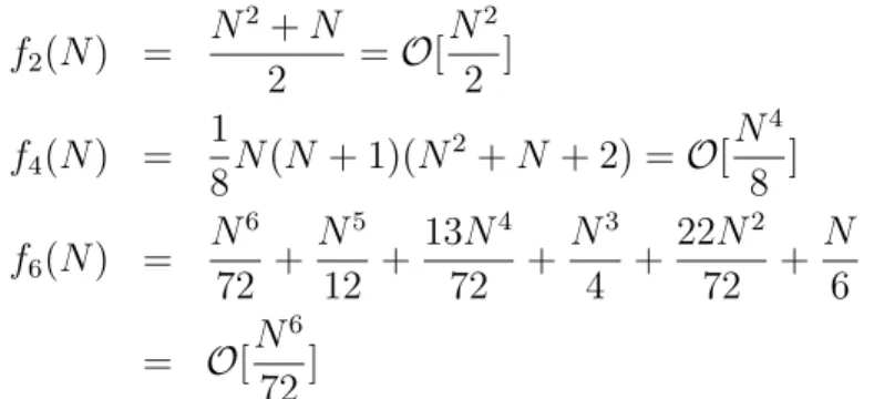
Finally, regarding cumulant estimation, the computation of the 2q-th order cumulant of a
N-dimensional random process requires (2q−1)K flops where K stands for the data length. Consequently, the number of flops required to compute the2q-th order cumulant array exploiting all its symmetries is then given by (2q−1)Kf2q(N) flops where f2q(N)denotes the number of its free entries and is given as a function of N, for q= 1,2,3, by:
f2(N) = N2+N 2 =O[ N2 2 ] f4(N) = 1 8N(N + 1)(N 2+N + 2) =O[N 4 8 ] f6(N) = N6 72 + N5 12 + 13N4 72 + N3 4 + 22N2 72 + N 6 = O[N 6 72]
Table I summarizes the numerical complexity of the elementary operations considered in this paper.
Numerical complexity (flops)
G=AB N2P
Lin. system solving 4N3/3
SVD ofA 2N2P+ 4N P2+ 14P3/3
EVD ofA 4N3/3
JAD [10] (Symmetric case) IN(N−1)(4N M+ 17M+ 4N+ 75)/2
Estimation of the2q-th (2q−1)Kf2q(N)
order cumulants array
EVD - based whitening KN2/2 + 4N3/3 +P N K
SVD - based whitening O[2KN2]
TABLE I
NUMERICAL COMPLEXITY OF ELEMENTARY OPERATIONS GENERALLY USED IN THEICAMETHODS.AANDBARE TWO
MATRICES OF SIZE(N×P)AND(P×N),RESPECTIVELY.IANDM STAND FOR THE NUMBER OF EXECUTED SWEEPS AND
THE NUMBER OF MATRICES TO BE JOINTLY DIAGONALIZED,RESPECTIVELY.f2q(N)DENOTES THE NUMBER OF FREE
Based on the complexity of these elementary operations, the numerical complexity of each of the fifteen ICA methods we have selected is given in table II. Again, we insist that a whitening procedure has been applied in all methods.
V. PERFORMANCE ANALYSIS ON SIMULATED DATA
Two experiments are considered in this section to evaluate the fifteen ICA algorithms in the context of epileptic signals (interictal spikes) corrupted by muscle artifacts. The first one uses synthetic spike-like epileptic EEG signals generated by realistic biomathematical models in order to quantify the performance of the methods. In the second experiment, real data are processed in order to get qualitative results. In the first experiment, the behavior of ICA methods is studied as a function of the Signal to Noise Ratio (SNR), for a fixed data length ofK = 8192
samples, which corresponds to 32 seconds. All reported results are obtained by averaging over 50 realizations the outputs of the performance criterion subsequently defined.
A. Data generation
The main purpose of this subsection is to explain how we obtain synthetic but realistic data for quantifying the performance of the methods. The simulated 32-channels EEG data (one observation is displayed in figure 1) are generated with a spatio-temporal model developed by our team [16]–[18]. In this model, EEG sources were represented as a dipole layer distributed over the cortical surface. The geometrical description of the cortical surface was achieved by using a mesh made of19626triangles (mean surface of4.8mm2) obtained from the segmentation of the gray-white matter interface from a patient 3D T1-weighted MRI. Each triangle of the mesh was associated to an elementary current dipole. The dipole was placed at the barycenter of the triangle and oriented perpendicular to its surface. The moment of each dipole was weighted by a coefficient proportional to the area of the corresponding triangle. In addition, each dipole was assumed to correspond to a distinct cortical neuronal population. Its time course, which represents the time-varying dynamics of the associated population, was provided by the output of a neuronal population model [54], in which parameters can be adjusted to generate either background-like activity or interictal-spikes. In this model the source of these epileptic activities was manually delineated on the mesh as a set of contiguous triangles. Dipoles associated with triangles within the patch were assigned highly correlated interictal spike activities (i.e. transient
Computational complexity
N: number of EEG electrodes,P: number of sources,iti, i∈ {1,· · ·,12}: number of iterations in PICA, InfoMax,
FastICAsym, FastICAdef, ERICA, SIMBEC, 4-CANDHAPc,Q: required complexity to compute the roots of a real
4-th degree polynomial by Ferrari’s technique in CoM2,Lw,Nt,Nf,M1andM2: smoothing window’s length, number of time bins, number of frequency bins, number of matrices referred to the time-frequency point wherein sources are of significant energy and number of matrices among thoseM1ones with only one active source in the
considered time-frequency point, respectively, in TFBSS,δωi= 1ifi∈ {2,· · ·,6}andδωi= 0otherwise.
SOBIrob M KN2/2 + 5M2N3−M3N3/3 + 2M N2P+M P2N+M P2+ (M P2+ 4P3/3)J1+M P+M N2+ 2N3/3 +N P+ (3N−P)P2/3 +IP(P−1)(17M+ 75 + 4P+ 4P M)/2 SOBI min{KN2/2 + 4N3/3 +P N K,2KN2}+ 4N3/3 + (M−1)N3/2 +IP(P−1)(17(M−1) + 75 + 4P+ 4P(M−1))/2 TFBSS min(KN2/2 + 4N3/3 +P N K+,2KN2) + 2Plog 2P+P+ (K+Lw+ log2(Lw))NtNfP(P+ 1)/2 + 2M1P3/3 + 3T2+IP(P−1)(4P M2+ 17M2+ 4P+ 75)/2 PICA min(KN2/2 + 4N3/3 +P N K,2KN2) + (P3+ (K+ 1)P2+ 3P K)it1 InfoMax min(KN2/2 + 4N3/3 +P N K,2KN2) + (P2+P3+ 4P+ 5KP)it2
FastICAdef min(KN2/2 + 4N3/3 +P N K,2KN2) + (2(P−1)(P+K) + 5KP(P+ 1)/2)it3
FastICAsym min(KN2/2 + 4N3/3 +P N K,2KN2) + 2N3/2 + (16P3/3 +P2+ 3KP2)it4
CoM2 min(KN2/2 + 4N3/3 +P N K,2KN2) +IP2Q/2 + min(12If4(P)P2 + 2IP3 + 3Kf4(P) + KP2,13IKP2/2)
JADE min(KN2/2 + 4N3/3 +P N K,2KN2) + 3Kf4(P) +KP2+ min(4P6/3,8P3(P2+ 3)) +IP(P−
1)(75 + 21P+ 4P2)/2 ERICA min(KN2/2 + 4N3/3 +P N K+,2KN2) +P N T+ 9P N2+113N3+N2+N+it7(P N T+ 5P2T+ 4P T+ 3P2+ 3P3+P2N) SIMBEC min(KN2/2 + 4N3/3 +P N K+,2KN2) +N2T+ 5P2+ 9P N2+11 3N 3+N2+N+it 5(P N T+ δω2(N P T +N P+P 2 N+P3) +δω3(2P T+N P T +N P +P 2 N+P3) +δω4(2P T+ 3N P T+ 2N P2+P3) +δ ω5(5P T+ 3N P T+N P 3+N P+ 2P2N+P3) +δ ω6(7P T+ 5N P T + 4N P 2+ P2N+P3) + 12P2+ 12P2N+22 3P 3 +N P)
FOBIUMJAD min(KN2/2 + 4N3/3 +P N K+,2KN2) + 3M Lf4(N) + 2N6/3 +P2(3N2−P)/3 + (M−1)N6/2 + IN2(N2−1){4N2(M−1) + 17(M−1) + 4N2+ 75}/2 + 2N3P ICAR min(KN2/2 + 4N3/3 +P N K+,2KN2) +K(3f4(N) + 2N6/3 +P2(3N2−P)/3 +N2P+ (8N P2+ 11N3/3 +N2+N)N+N2P2(N−1) +IP(P−1)(75 + 9N(N−1) + 8P N(N−1) + 4P) +IN(N− 1)(4N2+ 21N+ 75)/2 FOOBI1 min(KN2/2 + 4N3/3 +P N K+,2KN2) + 3Lf4(N) + 2N6/3 +P2(3N2−P)/3 +N2P+N2P2+ 2P(P+ 1)N4+ min{7M3m23+ 11m33/3,3M3m23}+IP(P−1)[4P2+ 21P+ 75]/2 +N2P(P+ 1) + min{6N3P,(2N3/3 + (3N−1)/3)P} 4-CANDHAPc min(KN2/2 + 4N3/3 +P N K+,2KN2) +9772N6+N2P2+ (3N2P2+38P N3+ 10P N+353P3− 2 3P)it12+P(IN(N−1)(8N+ 90))/2 TABLE II
interictal spikes) using an appropriate setting of coupling parameters between populations. All other dipoles of the cortical mesh were assigned a null activity. From this setup, we built a spatio-temporal source matrixS(e) containing the time-varying activities of all cortical epileptic dipoles. Thep-th line of this matrix contains the time-course of the p-th dipole within the patch. According to section II, matrix S(e) also represents one realization of the vector random process
{s(e)[k]} (1).
Scalp EEG data were then generated using a realistic head model representing the brain, the skull and the scalp [27]. From this head model, the forward problem was then numerically solved for each triangle within the patch using a boundary element method (ASA, ANT, Enschede, Netherlands) to obtain the leadfield matrix A(e) of equation (1). This mixing matrix gives the contribution of each dipole of the patch at the level of 32 scalp electrode positions (19-20 standard 10-20 electrodes plus additional electrodes at FC1, FC2, FC5, FC6, CP1, CP2, CP5, FT9, FT10, P9, P10 and POZ). The (N ×K) matrix X(e) of scalp epileptic data is thus given by X(e) = A(e)S(e). In this paper we considered a single patch, made of 100 contiguous triangles (5 cm2) located in the left superior temporal gyrus, where the activities of dipoles
within the patch were highly correlated. In addition, for each experiment and each trial, EEG muscle activity was extracted from real 32-channel EEG data in order to generate the matrix
X(b,m)=A(b)S(b)+A(m)S(m)+N of noisy scalp background and muscular activities, given in (1). More precisely, each trial of EEG muscle activity was normalized with respect to the channel showing the maximal power. Then, different levels of amplitude of noisy background and muscular activities were added to the simulated spike activities to get noisy simulated signals with different SNR values.
B. Performance criterion
The performance of the fifteen ICA methods has been evaluated by computing the following Normalized Mean-Squared Error (NMSE):
NMSE= N X n=1 PL `=1 PK k=1 xn(e)[k]−xˆ(ne,`)[k] 2 LPK k=1x (e) n [k] 2 (6)
where {x(ne)[k]} is the n-th row of the X(e) matrix defined in section V-A, {xˆ(ne,`)[k]} is the reconstructed surface EEG after denoising from the `-th run, L is the number of Monte Carlo
runs, K is the data length andN is the number of electrodes. More particularly, the independent components extracted by each method from the `-th run are classified in a descending order according to their respective autocorrelation values. As the autocorrelation of muscle artifacts is relatively low with respect to that of epileptic spikes, the independent components representing muscle artifacts are expected to be among the last components. In turn, components of interest are classified among the first components, which facilitates their visual selection. Then, the signal vector {xˆ(e,`)[k]} is reconstructed by keeping only the components accounting for the sources of interest (epileptic spikes).
C. Effect of SNR
The objective of this experiment is to i) evaluate the impact of SNR on the quality of source extraction and ii) to compare the numerical complexity of the fifteen algorithms. The data length,
K, is fixed to 8192 samples, the SNR values are equal to−30,−25,−20,−15,−10and−5dB, and the numberP of sources varies, in the rangeP ∈ {2,3,4,5,6,7,8,12,16,20,24,28,32}. For conciseness, we display in Figure 1 an example of EEG signals denoised by only three methods, namely TFBSS, CoM2 and InfoMax. In the original un-noisy EEG (figure 2, left), the spike-like activity was clearly visible at electrode T3 (facing the patch), whereas it is entirely buried in noisy data (figure 2, column 2). The spike activity at electrode T3 was well reconstructed with TFBSS, InfoMax and CoM2. However, for InfoMax and CoM2, the diffusion of this activity on other channels was slightly different than in original data. This difference is more visible when the TFBSS method is considered.
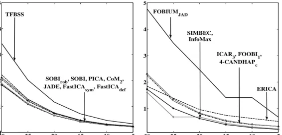
Figures 2 and 3 show the variations of NMSE and the numerical complexity of the fifteen methods as a function of SNR, respectively. Note that, in the following, the NMSE and the numerical complexity are only illustrated by choosing the value ofP yielding the best NMSE. In addition, the methods are classified into two main categories: i) methods with classical standard-ization, namely JADE, CoM2, SOBI, SOBIrob, PICA, FastICAsym, FastICAdef and TFBSS, and
ii) methods using a standardization without any reduction of dimension, namely FOBIUMJAD,
FOOBI1, ICAR3, 4-CANDHAPc, InfoMax, ERICA and SIMBEC.
From Figure 2, we can observe that JADE, CoM2, SOBI, SOBIrob, PICA, FastICAsym and
FastICAdef have a quasi-similar behaviour, whatever the SNR value. FOOBI1, ICAR3 and
of high SNR values (-10 and -5 dB). Regarding the FOBIUMJAD and TFBSS algorithms they
clearly show a poorer performance than that of the other algorithms. The SIMBEC method performs similarly to InfoMax for SNR values equal or higher than -20 dB and presents the best performance for an SNR lower than -20 dB. The ERICA method exhibits a performance similar to that of most of other algorithms for an SNR ranging from -30 dB to -25 dB, but becomes less efficient as the SNR of simulated data increases. Results obtained on methods of second category tend to demonstrate that using a standardization without any reduction of dimension as a preprocessing step forces the estimated mixing matrix to be well-conditionned.
The computational complexity (figure 3) is calculated by fixing the intrinsic parameters of each method according to those chosen to compute the NMSE criterion. In general, we can observe that, for each method, the numerical complexity is roughly stable, whatever the SNR values. More precisely, FOBIUMJAD, TFBSS and SIMBEC methods require the largest number of calculations.
These three methods are followed by PICA, ERICA, SOBI, SOBIrob, JADE, FastICAsym and
FOOBI1. Regarding the remaining algorithms (CoM2, FastICAdef, ICAR3, 4-CANDHAPc and
InfoMax), and more particularly CoM2, ICAR3, and InfoMax, they require a smaller amount of
calculations. These results can partially be explained by the number of independent components
P needed by each method to reach the best NMSE. Figure 4 indicates for each trial and for three SNR values (−30, −15 and −5 dB) the number P required by each method to obtain the best performance. We observe that all methods of the first category (JADE, CoM2, SOBI, SOBIrob,
PICA, FastICAsym, FastICAdef and TFBSS), ERICA, SIMBEC and InfoMax generally require
the extraction of P = 32independent components to obtain the best performance, whereas most of methods of second category, namely FOBIUMJAD, FOOBI1, ICAR3 and 4-CANDHAPc need
a smaller number of independent components to reach an equivalent performance.
The NMSE and the numerical complexity calculations of the fifteen methods indicate, in the simulated context of epileptic signals (interictal spikes) corrupted by muscle artifacts, that: i) InfoMax generally presents the best performance in the sense of NMSE criterion, ii) CoM2
offers the best NMSE versus numerical complexity compromise, and iii) FOBIUMJAD and
O2 P4 T6 C4 T4 F4 F8 FP2 PZ CZ FZ O1 P3 T5 C3 T3 F3 F7 FP1 O2 P4 T6 C4 T4 F4 F8 FP2 PZ CZ FZ O1 P3 T5 C3 T3 F3 F7 FP1 O2 P4 T6 C4 T4 F4 F8 FP2 PZ CZ FZ O1 P3 T5 C3 T3 F3 F7 FP1 O2 P4 T6 C4 T4 F4 F8 FP2 PZ CZ FZ O1 P3 T5 C3 T3 F3 F7 FP1 O2 P4 T6 C4 T4 F4 F8 FP2 PZ CZ FZ O1 P3 T5 C3 T3 F3 F7 FP1
Muscule activity (SNR=-25 dB) Simulated
EEG InfoMax Noisy EEG CoM 2 TFBSS Fig. 1. Example of denoising obtained in the case of simulated data: i) noise free simulated EEG (column 1), ii) noisy EEG after adding real musc le acti vity with SNR = -25 dB (column 2), iii) EEG denoised by Infomax (column 3), iv) EEG denoised by CoM 2 (column 4), and v) EEG denoised by TFBSS (column 5)
-300 -25 -20 -15 -10 -5 1 2 3 4 5 SNR (dB) N M S E -30 -25 -20 -15 -10 -5 1 2 3 4 5 SNR (dB) FOBIUM JAD TFBSS SIMBEC, InfoMax ERICA SOBI
rob, SOBI, PICA, CoM2,
JADE, FastICA
sym, FastICAdef
ICAR
3, FOOBI1,
4-CANDHAP
c
Fig. 2. NMSE as a function of SNR forK= 8192data samples taking the numberP of independent components such that each method gives the best NMSE
-30 -25 -20 -15 -10 -5 109 1010 1011 1012 SNR -30 -25 -20 -15 -10 -5 109 1010 1011 1012 SNR lo g 10 (C om pl ex it y) SOBI, PICA, FastICA sym TFBSS JADE FastICA def CoM 2 FOBIUM JAD SIMBEC ERICA 4-CANDHAP c ICAR3 InfoMax SOBI rob FOOBI 1
Fig. 3. Numerical complexity as a function of SNR forK= 8192data samples taking the numberPof independent components such that each method gives the best NMSE
2 4 6 8 16 24 32 0 25 50 2 4 6 8 16 24 32 0 25 50 2 4 6 8 16 24 32 0 25 50 2 4 6 8 16 24 32 0 25 50 2 4 6 8 16 24 32 0 25 50 2 4 6 8 16 24 32 0 25 50 2 4 6 8 16 24 32 0 25 50 2 4 6 8 16 24 32 0 25 50 2 4 6 8 16 24 32 0 25 50 2 4 6 8 16 24 32 0 25 50 2 4 6 8 16 24 32 0 25 50 2 4 6 8 16 24 32 0 25 50 2 4 6 8 16 24 32 0 25 50 2 4 6 8 16 24 32 0 25 50 2 4 6 8 16 24 32 0 25 50
L
L
L
P P P P JADE P CoM 2 TFBSS SOBI ro b PICA FastICA sym FastICA def SOBI FOBIUM JAD FOOBI 1 ICAR 3 4-CANDHAP c InfoMax ERICA SIMBEC Fig. 4. Histogram of the number P of independent components required by each method to obtain the best NMSE: i) SNR equal to − 30 dB (blue bar), ii) SNR equal to − 15 dB (green bar), and iii) SNR equal to − 5 dB (gre y bar)VI. APPLICATION TO REAL DATA
In this section we propose to test the feasibility of ICA algorithms on real data. For conciseness, only results given by TFBSS, CoM2 and InfoMax are shown. It is worth noting that these three methods were marked out by their results on simulated EEG data in terms of NMSE and numerical complexity in the previous section. The three methods were applied to the denoising of interictal spikes in a patient suffering from drug-resistant partial epilepsy. As part of his presurgical evaluation, this patient underwent two sessions of video-EEG monitoring, brain Magnetic Resonance Imaging (MRI), as well as interictal and ictal Single-Photon Emission Computed Tomography (SPECT) acquisition. During video-EEG monitoring, scalp-EEG data were acquired from 32 electrodes (19-20 standard 10-20 electrodes plus additional electrodes at FC1, FC2, FC5, FC6, CP1, CP2, CP5, FT9, FT10, P9, P10 and POZ) at a sampling frequency of 256 Hz.
These data were reviewed in order to isolate three epochs: i) two epochs containing a clean spike (figure 5, first and second column), and ii) one epoch including spikes hidden in muscle activity with very high level of noise (figure 5, third column). The same procedure as for simulated data was applied to reconstruct the denoised EEG signals. In addition, to evaluate the qualitative performance of the three methods, a source localization was performed on the two original cleaned signals (considered as a reference), on the noisy data, as well as on the latter data denoised by TFBSS, CoM2 and InfoMax, respectively. The recent 4-ExSo-MUSIC
algorithm [7] was used to achieve the source localization. Figure 5 illustrates that interictal spikes were visible at electrodes F8, T4, FC5, and FT10 of the two epochs of clean data (columns 1 and 2), whereas they were hidden in the noisy data (column 3). Clearly, the three ICA-methods enhance the interictal spikes at F8, T4, FC5, and FT10 electrodes and do not increase the diffusion of spikes on the remaining electrodes. We also calculated the numerical complexity of TFBSS, CoM2 and showed (in agreement to the simulated results) that CoM2 required the
smallest amount of calculations (about 8.107 flops), InfoMax used about4.109 flops and TFBSS
needed a larger amount of calculations (about 2.1012 flops).
Regarding the source localization results (bottom of each column of figure 5), the spikes were localized in the right anterior temporal region for the first epoch of clean data (column 1) and both in the right temporal neocortex and in the right insula for the second epoch of clean data (column
2). Even if these localizations were slightly different, they were in general consistent with the visual interpretation of T1-weighted MRI data and also corroborated by interictal SPECT data. For the noisy epoch (column 3), the spike source was incorrectly localized in the left temporal region. Spike data denoised by CoM2 were localized both in the right temporal neocortex and
in the right insula in agreement with the source localization obtained from the second epoch of clean data. The localization results at the output of InfoMax and TFBSS were quasi-similar with those obtained from the second epoch of clean data.
The results obtained on real interictal epileptic spikes suggest that choosing the appropriate ICA method for processing actual data in the context of interictal epileptic spikes is not an easy task. Indeed, it is not obvious to know the true epileptic area with a perfect accuracy, since two clean epochs recorded in the same patient can lead to slightly different source locations. Consequently, it is clearly not possible to say which ICA method denoises better the epileptic spikes on real data, since the source localization after each ICA-based denoising is consistent with that obtained from one of both epochs of clean data. In terms of performance, we can just say that each of our tested ICA methods is doing its work properly, i.e. it removes successfully the muscle artifacts without altering the interictal epileptic spikes, and it significantly improves the quality of the source localization. As far as the numerical complexity is considered, CoM2
P O Z P O Z P O Z P O Z P 1 0 P 1 0 P 1 0 P 1 0 P 9 P 9 P 9 P 9 F T 1 0 F T 1 0 F T 1 0 F T 1 0 F T 9 F T 9 F T 9 F T 9 C P 6 C P 6 C P 6 C P 6 C P 5 C P 5 C P 5 C P 5 F C 5 F C 5 F C 5 F C 5 F C 6 F C 6 F C 6 F C 6 C P 2 C P 2 C P 2 C P 2 C P 1 C P 1 C P 1 C P 1 F C 2 F C 2 F C 2 F C 2 F C 1 F C 1 F C 1 F C 1 P Z P Z P Z P Z C Z C Z C Z C Z F Z F Z F Z F Z T 6 T 6 T 6 T 6 T 5 T 5 T 5 T 5 T 4 T 4 T 4 T 4 T 3 T 3 T 3 T 3 F 8 F 8 F 8 F 8 F 7 F 7 F 7 F 7 O 2 O 2 O 2 O 2 O 1 O 1 O 1 O 1 P 4 P 4 P 4 P 4 P 3 P 3 P 3 P 3 C 4 C 4 C 4 C 4 C 3 C 3 C 3 C 3 F 4 F 4 F 4 F 4 F 3 F 3 F 3 F 3 F P 2 F P 2 F P 2 F P 2 F P 1 F P 1 F P 1 F P 1 P O Z P O Z P O Z P O Z P 1 0 P 1 0 P 1 0 P 1 0 P 9 P 9 P 9 P 9 F T 1 0 F T 1 0 F T 1 0 F T 1 0 F T 9 F T 9 F T 9 F T 9 C P 6 C P 6 C P 6 C P 6 C P 5 C P 5 C P 5 C P 5 F C 5 F C 5 F C 5 F C 5 F C 6 F C 6 F C 6 F C 6 C P 2 C P 2 C P 2 C P 2 C P 1 C P 1 C P 1 C P 1 F C 2 F C 2 F C 2 F C 2 F C 1 F C 1 F C 1 F C 1 P Z P Z P Z P Z C Z C Z C Z C Z F Z F Z F Z F Z T 6 T 6 T 6 T 6 T 5 T 5 T 5 T 5 T 4 T 4 T 4 T 4 T 3 T 3 T 3 T 3 F 8 F 8 F 8 F 8 F 7 F 7 F 7 F 7 O 2 O 2 O 2 O 2 O 1 O 1 O 1 O 1 P 4 P 4 P 4 P 4 P 3 P 3 P 3 P 3 C 4 C 4 C 4 C 4 C 3 C 3 C 3 C 3 F 4 F 4 F 4 F 4 F 3 F 3 F 3 F 3 F P 2 F P 2 F P 2 F P 2 F P 1 F P 1 F P 1 F P 1 P O Z P O Z P O Z P O Z P 1 0 P 1 0 P 1 0 P 1 0 P 9 P 9 P 9 P 9 F T 1 0 F T 1 0 F T 1 0 F T 1 0 F T 9 F T 9 F T 9 F T 9 C P 6 C P 6 C P 6 C P 6 C P 5 C P 5 C P 5 C P 5 F C 5 F C 5 F C 5 F C 5 F C 6 F C 6 F C 6 F C 6 C P 2 C P 2 C P 2 C P 2 C P 1 C P 1 C P 1 C P 1 F C 2 F C 2 F C 2 F C 2 F C 1 F C 1 F C 1 F C 1 P Z P Z P Z P Z C Z C Z C Z C Z F Z F Z F Z F Z T 6 T 6 T 6 T 6 T 5 T 5 T 5 T 5 T 4 T 4 T 4 T 4 T 3 T 3 T 3 T 3 F 8 F 8 F 8 F 8 F 7 F 7 F 7 F 7 O 2 O 2 O 2 O 2 O 1 O 1 O 1 O 1 P 4 P 4 P 4 P 4 P 3 P 3 P 3 P 3 C 4 C 4 C 4 C 4 C 3 C 3 C 3 C 3 F 4 F 4 F 4 F 4 F 3 F 3 F 3 F 3 F P 2 F P 2 F P 2 F P 2 F P 1 F P 1 F P 1 F P 1 T im e ( s e c o n d s )
C
le
a
n
d
a
ta
1
C
le
a
n
d
a
ta
2
N
o
is
y
d
a
ta
In
fo
M
a
x
C
o
M
2T
F
B
S
S
Fig. 5. Denoising of real interictal spik es data: i) tw o noise-free interictal spik es (columns 1 and 2), ii) epoch including spi k es hidden in muscle acti vity with v ery high le v el of noise (column 2), iii) EEG denoised by Infomax, CoM 2 and TFBSS (columns 3, 4 and 5, respecti v ely). The source localization results at the output of 4-ExSo-MUSIC are depicted at the bottom of each column.VII. CONCLUSION
Advanced epilepsy research and diagnosis require precise information, which can be extracted from non-invasive EEG data. However, EEG signals may be unfortunately contaminated by instrumental noise and various electrophysiological artifacts, such as power line noise, broken wire contacts, ocular movements and muscular activity. These types of noise and artifacts hide physiological activities of interest. Among all these artifacts, the muscular activity is particularly difficult to remove. Previous investigations in the biomedical engineering context showed that ICA is an efficient approach for the blind extraction of components of interest from a noisy mixture of sources. Nevertheless, the application of ICA to the extraction of epileptic signals in the presence of muscular activities is still challenging; it is indeed difficult to access a ground truth for epileptic sources in order to evaluate the accuracy of ICA. In addition, most of the studies that have used ICA to analyze and to process epileptic signals have only explored a limited number of ICA algorithms, namely InfoMax, FastICA and SOBI. These issues are addressed in this paper through the comparison of fifteen ICA algorithms, both in terms of performance and numerical complexity. The comparative analysis is first performed on simulated EEG data, reproducing realistic epileptic EEG signals contaminated by muscle artifacts, in order to quantify the accuracy of the ICA methods. CoM2 then appears as the ICA method offering the best compromise
between performance and numerical complexity, while TFBSS and FOBIUMJADoffer the worse.
The good behavior of CoM2 is next confirmed on one set of real data. Forthcoming work will
aim first at comparing even more ICA methods, for instance by including improved versions of the techniques analyzed in [36], [56]. Second, we will acquire dense EEG data (>128channels) in order to analyze the performance of ICA methods as a function of the number of electrodes.
VIII. ACKNOWLEDGMENT
This work has been partly supported by the French ANR contract 10- BLAN-MULTIMODEL.
REFERENCES
[1] L. ALBERA, P. COMON, L. PARRA, A. KARFOUL, A. KACHENOURA, and L. SENHADJI, “Biomedical applications,”
inHandbook of blind source separation, P. COMON and C. JUTTEN, Eds. Academic Press, March 2010.
[2] L. ALBERA, A. FERREOL, P. CHEVALIER, and P. COMON, “ICAR: Independent Component Analysis using Redun-dancies,” in ISCAS 04, 2004 IEEE International Symposium on Circuits and Systems, Vancouver, Canada, May 23-26 2004.
[3] ——, “ICAR, a tool for blind source separation using fourth order statistics only,”IEEE Transactions On Signal Processing, vol. 53, pp. 3633–3643, October 2005.
[4] S. AMARI, “Natural gradient works efficienttly in learning,”Neural Computation, vol. 10, no. 2, pp. 251–276, 1998. [5] A. BELOUCHRANI, K. ABED-MERAIM, J. F. CARDOSO, and E. MOULINES, “A blind source separation technique
using second-order statistics,”IEEE Transactions On Signal Processing, vol. 45, no. 2, pp. 434–444, 1997.
[6] A. BELOUCHRANI and A. CICHOCJI, “Robust whitening procedure in blind source separation context,” Electronics
Letters, vol. 23, no. 24, pp. 2050–2051, 2000.
[7] G. BIROT, L. ALBERA, F. WENDLING, and I. MERLET, “Localisation of extended brain sources from eeg/meg: the exso-music approach,”Elsevier Neuroimage, vol. 56, no. 1, pp. 102–113, May 2011.
[8] J. F. CARDOSO, “Blind signal separation: statistical principles,”Proceedings of the IEEE, vol. 9, no. 10, pp. 2009–2025, Oct. 1998.
[9] J. F. CARDOSO and A. SOULOUMIAC, “Blind beamforming for non-gaussian signals,”IEE Proceesings-F, vol. 140, no. 6, pp. 362–370, Dec. 1993.
[10] ——, “Jacobi angles for simultaneous diagonalization,”SIAM Journal Matrix Analysis and Applications, vol. 17, no. 1, pp. 161–164, 1996.
[11] T. F. CHAN, “An improved algorithm for computing the singular value decomposition,”ACM Transaction on Mathematical
Software, vol. 8, no. 1, pp. 72–83, Mar. 1982.
[12] P. COMON, “Separation de melanges de signaux,” inGRETSI 89, Douzième colloque sur le Traitement du Signal et des
Images, Juan les Pins, June 12-16 1989, pp. 137–140.
[13] ——, “Independent Component Analysis, a new concept ?”Signal Processing, Elsevier, vol. 36, no. 3, pp. 287–314, 1994. [14] P. COMON and C. JUTTEN, “Handbook of blind source separation.” Academic Press, March 2010.
[15] P. COMON, X. LUCIANI, and A. L. F. D. ALMEIDA, “Tensor decompositions, alternating least squares and other thales,”
Journal of Chemometrics, vol. 23, 2009.
[16] D. COSANDIER-RIMELE, J. M. BADIER, P. CHAUVEL, and F. WENDLING, “A physiologically plausible spatio-temporal model for depth-EEG signals recorded with intracerebral electrodes in human partial epilepsy,”IEEE Transactions
On Biomedical Engineering, vol. 3, no. 54, pp. 380–388, February 2007.
[17] D. COSANDIER-RIMELE, I. MERLET, J. M. BADIER, P. CHAUVEL, and F. WENDLING, “The neuronal sources of EEG: Modeling of simultaneous scalp and intracerebral recordings in epilepsy,”NeuroImage, vol. 42, no. 1, pp. 135–146, April 2008.
[18] D. COSANDIER-RIMELE, I. MERLET, F. BARTOLOMEI, J. M. BADIER, and F. WENDLING, “Computational modeling of epileptic activity: from cortical sources to eeg signals,”Journal of clinical neurophysiology, vol. 27, no. 6, pp. 465–470, December 2010.
[19] S. CRUCES, L. CASTEDO, and A. CICHOCKI, “Novel blind source separation algorithms using cumulants,” in
Proceedings on International Conference on Acoustic, Speech and Signal Processing (ICASSP’2000), 2000, pp. 3152–3155.
[20] S. A. CRUCES-ALVEREZ, A. CICHOCKI, and S. AMARI, “On a new blind signal extraction algorithm: different criteria and stability analysis,”IEEE Signal Processing Letters, vol. 9, no. 8, pp. 233–236, 2002.
[21] Y. DEVILLE, C. JUTTEN, and R. VIGARIO, “Overview of source separation applications,” inHandbook of blind source
separation, P. COMON and C. JUTTEN, Eds. Academic Press, March 2010.
(FOBIUM),” inICASSP 03, 2003 IEEE International Conference on Acoustics Speech and Signal Processing, Hong Kong, China, April 6-10 2003, pp. 41–44.
[23] ——, “Fourth order blind identification of underdetermined mixtures of sources (FOBIUM),”IEEE Transactions On Signal
Processing, vol. 53, pp. 1254–1271, April 2005.
[24] C. FEVOTTE and C. DONCARLI, “Two contributions to blind sources separation using time-frequency distributions,”
IEEE Signal processing Letters, vol. 11, no. 3, pp. 386–389, Mar. 2004.
[25] G. H. GOLUB and C. F. V. LOAN,Matrix computations, second edition. The Johns Hopkins University Press, Baltimore, MD, 1989.
[26] G. H. GOLUB and C. REINSCH,Singular value decomposition and least squares solutions. In Handbook for Automatic
computation II, Linear Algebra, J. H. WILKINSON. Springer-Verlag, New York, 1970.
[27] S. I. GONCALVES, J. C. D. MUNCK, J. P. A. VERBUNT, F. BIJMA, R. M. HEETHAAR, and F. L. D. SILVA, “In vivo measurement of the brain and skull resistivities using an EIT-based method and realistic models for the head,”IEEE
Transactions on Biomedical Engineering, vol. 50, no. 6, pp. 754–767, 2003.
[28] A. HYVARINEN, “Fast and robust fixed-point algorithms for independent component analysis,”IEEE Transactions On
Neural Networks, vol. 10, no. 3, pp. 626–634, 1999.
[29] T.-P. JUNG, C. HUMPHRIES, T. W. LEE, S. MAKEIG, M. J. MCKEOWN, V. IRAGUI, and T. J. SEJNOWSKI, “Extended ica removes artifacts from electroencephalographic recordings,”Advances in Neural Information Processing Systems, vol. 10, 1998.
[30] T. P. JUNG, S. MAKEIG, M. WESTERFIELD, J. TOWNSEND, E. COURCHESNE, and T. J. SEJNOWSKI, “Independent component analysis of single-trial even-related potentials,” in ICA’99, Second International Symposium on Independent
Component Analysis and Blind Signal Separation, Aussois, France, Jan. 1999, pp. 173–178.
[31] A. KACHENOURA, L. ALBERA, and L. SENHADJI, “SÈparation aveugle de sources en ingÈnierie biomÈdicale,”IRBM,
Elsevier, vol. 28, no. 1, pp. 20–34, March 2007.
[32] A. KACHENOURA, L. ALBERA, L. SENHADJI, and P. COMON, “ICA: a potential tool for BCI systems,”IEEE Signal
Processing Magazine, special issue on Brain-Computer Interfaces, vol. 25, no. 1, pp. 57–68, 2008.
[33] A. KARFOUL, L. ALBERA, and L. DE LATHAUWER, “Canonical decomposition of even higher order cumulant arrays for blind underdetermined mixture identification,” inSAM 08, Fifth IEEE Workshop on Sensor Array and Multi-Channel
Signal Processing, Darmstadt, Germany, 21-23 July 2008, pp. 501–505.
[34] ——, “Iterative methods for the canonical decomposition of multi-way arrays: Application to blind underdetermined mixture identification,”Signal Processing, Elsevier, vol. 91, no. 8, pp. 1789–1802, August 2011.
[35] J. KARVANEN and V. KOIVUNEN, “Blind separation methods based on pearson system and its extensions,” Signal
Processing, Elsevier, vol. 82, pp. 663–673, 2002.
[36] Z. KOLDOSKY, P. TICHAVSKY, and E. OJA, “Efficient Variant of Algorithm FastICA for Independent Component Analysis Attaining the Cramér-Rao Lower Bound,” Efficient Variant of Algorithm FastICA for Independent Component
Analysis Attaining the Cramér-Rao Lower Bound, vol. 17, no. 5, pp. 1265–1277, 2006.
[37] L. D. LATHAUWER and J. CASTAING, “Blind identification of underdetermined mixtures by simultaneous matrix diagonalization,”IEEE Transactions on Signal Processing, vol. 56, no. 3, 2008.
[38] L. D. LATHAUWER, J. CASTAING, and J. F. CARDOSO, “Fourth-order cumulant-based blind identification of underdetermined mixtures,”IEEE Transactions on Signal Processing, vol. 55, no. 6, pp. 2965–2973, 2007.
[39] T. W. LEE, M. GIROLAMI, and T. J. SEJNOWSKI, “Independent component analysis using an extended infomax algorithm for mixed sub-gaussian and super-gaussian sources,”Neural Computation, vol. 11, no. 2, pp. 417–441, 1999.
[40] V. P. LEONOV and A. M. SHIRYAEV, “On a method of calculation of semi-invariants,”Theory of Probability and its
Applications, vol. 4, pp. 319–29, 1959.
[41] X. LUCIANI and L. ALBERA, “Joint eigenvalue decomposition using polar matrix factorization,” in Latent Variable
Analysis and Signal Separation LVA-ICA 2010, ser. Lecture Notes in Computer Science, vol. 6365. Saint Malo France:
Springer, September 2010, pp. 612–619.
[42] S. MAKEIG, A. J. BELL, T.-P. JUNG, and T. J. SEJNOWSKI, “Independent component analysis of electroencephalographic data,”Advances in Neural Information Processing Systems, vol. 8, pp. 145–151, 1996.
[43] S. MAKEIG et al., “EEGLAB: ICA Toolbox for Psychophysiological Research,”WWW Site, Swartz Center for
Compu-tational Neuroscience, Institute of Neural Computation, University of San Diego California <www.sccn.ucsd.edu/eeglab/>,
2000.
[44] P. MCCULLAGH,Tensor Methods in Statistics. Chapman and Hall, Monographs on Statistics and Applied Probability, 1987.
[45] B. W. MCMENAMIN, A. J. SHACKMAN, J. S. MAXWELL, D. R. BACHHUBER, A. M. KOPPENHAVER, L. L. GREISCHAR, and R. J. DAVIDSON, “Validation of ICA-based myogenic artifact correction for scalp and source-localized EEG,”NeuroImage, vol. 49, no. 3, pp. 2416 – 2432, 2010.
[46] E. MOREAU, “Criteria for complex sources separation,” inEUSIPCO 96, XIV European Signal Processing Conference, Triestre, Italy, September 1996, pp. 931–934.
[47] S. OLBRICH, J. JODICKE, C. SANDER, H. HIMMERICH, and U. HEGERL, “ICA-based muscle artefact correction of EEG data: What is muscle and what is brain?: Comment on McMenamin et al.”NeuroImage, vol. 54, no. 1, pp. 1 – 3, 2011.
[48] F. POREE, A. KACHENOURA, H. GAUVRIT, C. MORVAN, G. CARRAULT, and L. SENHADJI, “Blind source separation for ambulatory sleep recording,”Transactions on Information Technology in Biomedicine, vol. 10, no. 2, pp. 293–301, Apr. 2006.
[49] J. J. RIETA, F. CASTELLS, C. SANCHEZ, V. ZARZOSO, and J. MILLET, “Atrial activity extraction for atrial fibrillation analysis using blind source separation,”IEEE Transactions on Biomedical Engineering, vol. 51, no. 7, pp. 1176–1186, July 2004.
[50] J. SARVAS, “Basic mathematical and electromagnetic concepts of the biomagnetic inverse problems,”Physics in Medicine
and Biology, vol. 32, pp. 11–22, 1987.
[51] R. VIGARIO and E. OJA, “BSS and ICA in neuroinformatics: From current practices to open challenges,”IEEE Reviews
in Biomedical Engineering, vol. 1, pp. 50–61, 2008.
[52] R. VIGARIO, J. SARELA, V. JOUSMAKI, M. HAMALAINEN, and E. OJA, “Independent component approach to the analysis of EEG and MEG,”IEEE Transactions On Biomedical Engineering, vol. 47, no. 5, pp. 589–593, May 2000. [53] S. VOROBYOV and A. CICHOCKI, “Blind noise reduction for multisensory signals using ICA and subspace filtering,
with application to eeg analysis,”Biological Cybernetics, vol. 86, no. 4, pp. 293–3034, 2002.
[54] F. WENDLING, J. BELLANGER, F. BARTHOLOMEI, and P. CHAUVEL, “Relevance of nonlinear lumped-parameter models in the analysis of depth-eeg epileptic signals,” vol. 83, 2000, pp. 367–78.
[55] T. Y. YOUNG and T. W. CALVERT, Classification, estimation and pattern recognition. American Elsevier Publishing Company, 1974.
[56] A. YEREDOR, “Blind separation of Gaussian sources via second-order statistics with asymptotically optimal weighting,”
IEEE Signal Processing Letters, vol. 7, pp. 197–200, July 2000.
[57] V. ZARZOSO and A. HYVARINEN, “Iterative algorithms,” in Handbook of Blind Source Separation, P. Comon and C. Jutten, Ed. London, UK: Academic Press, 2010, ch. 6, pp. 179–225.
[58] A. ZIEHE and K. R. MULLER, “TDSEP - an efficient algorithm for blind separation using time structure,” inICANN’98,