Contents lists available atScienceDirect
Computers and Electronics in Agriculture
journal homepage:www.elsevier.com/locate/compagAutomatic detection and classi
fi
cation of honey bee comb cells using deep
learning
Thiago S. Alves
a,b,⁎, M. Alice Pinto
c, Paulo Ventura
c, Cátia J. Neves
c, David G. Biron
d,
Arnaldo C. Junior
b, Pedro L. De Paula Filho
b, Pedro J. Rodrigues
a,⁎aResearch Center in Digitalization and Intelligent Robotics (CeDRI), Instituto Politécnico de Bragança, Campus de Santa Apolónia, 5300-253 Bragança, Portugal bDepartment of Computer Science, Federal Technological University of Paraná (UTFPR), Medianeira, Paraná, Brazil
cCentro de Investigação de Montanha (CIMO), Instituto Politécnico de Bragança, Campus de Santa Apolónia, 5300-253, Portugal
dLaboratoire Microorganismes: Génome et Environnement, UMR CNRS 6023, Université Clermont-Auvergne, Campus Universitaire des Cézeaux, France
A R T I C L E I N F O Keywords:
Cell classification
Apis melliferaL. Semantic segmentation Machine learning Deep learning DeepBeesoftware A B S T R A C T
In a scenario of worldwide honey bee decline, assessing colony strength is becoming increasingly important for sustainable beekeeping. Temporal counts of number of comb cells with brood and food reserves offers re-searchers data for multiple applications, such as modelling colony dynamics, and beekeepers information on colony strength, an indicator of colony health and honey yield. Counting cells manually in comb images is labour intensive, tedious, and prone to error. Herein, we developed a free software, namedDeepBee©, capable of au-tomatically detecting cells in comb images and classifying their contents into seven classes. By distinguishing cells occupied by eggs, larvae, capped brood, pollen, nectar, honey, and other, DeepBee© allows an un-precedented level of accuracy in cell classification. Using Circle Hough Transform and the semantic segmen-tation technique, we obtained a cell detection rate of 98.7%, which is 16.2% higher than the best result found in the literature. For classification of comb cells, we trained and evaluated thirteen different convolutional neural network (CNN) architectures, including: DenseNet (121, 169 and 201); InceptionResNetV2; InceptionV3; MobileNet; MobileNetV2; NasNet; NasNetMobile; ResNet50; VGG (16 and 19) and Xception. MobileNet revealed to be the best compromise between training cost, with ~9 s for processing all cells in a comb image, and accuracy, with an F1-Score of 94.3%. We show the technical details to build a complete pipeline for classifying and counting comb cells and we made the CNN models, source code, and datasets publicly available. With this effort, we hope to have expanded the frontier of apicultural precision analysis by providing a tool with high performance and source codes to foster improvement by third parties ( https://github.com/AvsThiago/DeepBee-source).
1. Introduction
In a scenario of worldwide honey bee (Apis mellifera L.) decline, assessing colony strength is becoming increasingly important as it can assist apiary management strategies and provide valuable information for research purposes. Counts of comb cells with brood and food re-serves offer beekeepers information on colony nutritional status, colony health status, queen quality, honey yield, etc. The same data collected across time can be used by researchers in multiple applications, in-cluding assessment of queen genotypes, assessment of new treatments against parasites and pathogens, modelling colony dynamics in re-sponse to abiotic (pesticides) or biotic (parasites, pathogens, predators) stressors, among others.
Delaplane et al. (2013)reviewed the methods for assessing colony strength, among which is the Liebefeld method. This method has been included in the HEALTHY-B toolbox compiled by EFSA (European Food Safety Authority) for harmonising data collection on the health status of honey bees in Europe (EFSA AHAW Panel, 2016). The Liebefeld method is based on direct observations of comb frames in the apiary. Estimates are made with the help of an eight-quadrant grid placed in front of each frame. With the grid in place, the observer estimates the surface oc-cupied by the targeted class (e.g., honey or capped brood) in every quadrant. This method is prone to error, time-consuming and produces data with a high level of subjectivity. Additionally, at least two well-trained observers are required for gathering the data and for obtaining better estimates through averaging the two subjective evaluations
https://doi.org/10.1016/j.compag.2020.105244
Received 29 April 2019; Received in revised form 13 November 2019; Accepted 22 January 2020 ⁎Corresponding authors at: Rua Mário Fontana, 1331, Toledo, Paraná CEP: 85910-190, Brazil.
E-mail addresses:[email protected](T.S. Alves),[email protected](M.A. Pinto),[email protected](C.J. Neves),[email protected](D.G. Biron), [email protected](A.C. Junior),[email protected](P.L. De Paula Filho),[email protected](P.J. Rodrigues).
Available online 03 February 2020
0168-1699/ © 2020 Elsevier B.V. All rights reserved.
lows edition of the automatic predictions, if needed, and produces a spreadsheet file for downstream analysis. While developing this tool, we further contributed to a wider community including machine learning, image processing and other software developers (i) by pro-viding a method in the segmentation process to automatically readjust the scale of the images driven by the size of the cells, (ii) by testing different neural network architectures related to performance and quality of results, (iii) by providing datasets that can be employed by others when testing new methods, and (iv) by making available the source codes enabling the reproducibility of our results.
1.1. Motivation
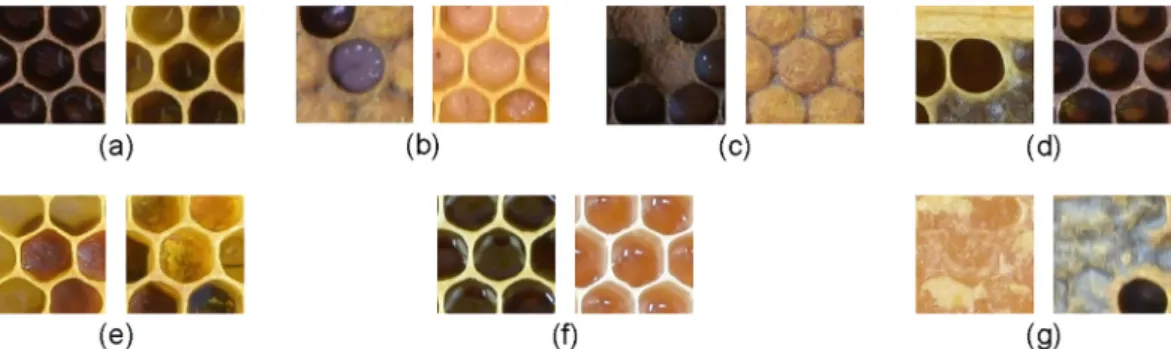
Several semi-automatic methods for assessing colony strength using digital images of comb frames have been proposed in the last years (reviewed below). When compared with manual methods, post-hoc analysis of comb images reduces the time of information collection, provides more accurate data, and assures reproducibility of results even with different users. Furthermore, the images themselves are perma-nent records of the data, representing an important step towards more accountable and objective assessment of colony strength, as no record is usually available after the commonly used visual estimation of combs. Developing tools for analysis of comb images requires pre-defining the cell classes that will be targeted. The higher the number of cell classes to be distinguished in a comb image, the greater the complexity of the classification model. During a colony lifetime, comb cells may be (i) momentarily empty, (ii) occupied by the honey bee in its different immature stages (egg, larva, pupa), or (iii)filled with food resources (pollen, nectar, honey) required for colony development and main-tenance (Fig. 1). To reflect the high level of cell-content diversity, at least seven different classes should be pre-defined when developing models for cell classification. In addition to class diversity, there might be a wide array of colours and textures within each class, making cell classification a challenging endeavour.
Previous works (reviewed below) have addressed this challenge by developing tools for assessing only the number of capped brood cells (Fig. 1c), a task that is greatly facilitated by the striking visual differ-ences between capped brood and the remaining cells. Here, we devel-oped a tool capable of assigning cell contents to seven different classes, which represents an unprecedented level of accuracy in classification of comb images.
created for the image processing softwareImageJ(https://imagej.nih. gov/ij/index.html). With this plugin, the user is able to open the pre-viously segmented image and calculate automatically the area occupied by both capped and uncapped cells.
Cornelissen et al. (2009)further advanced comb image assessment by developing a semi-automatic method that counted the number of capped brood cells, instead of measuring occupied area. This method was on average 23 s slower than the Liebefeld method, as it required human intervention during segmentation. However, the estimates of capped cells were more accurate with the semi-automatic method (correlation with the actual number of cells = 0.99) than with the Liebefeld method (correlation with the actual number of cells = 0.91). One of thefirst digital methods capable of detecting and counting individual cells was developed byLiew et al. (2010). The authors used pre-processing methods to highlight the edges and applied the Circle Hough Transform (CHT) to detect the cells. They obtained a detector with a cell detection rate of 82.6%.
More recently,Rodrigues et al. (2016)developed a method for au-tomatic detection and counting of capped brood cells using circular convolution. The circular mask has the same size of a comb cell, it stops in each cell position, and it calculates the contrast between the pixels of the cell edge and its interior. From this contrast, it is possible to know whether there is a cell, and according to established thresholds, it is possible to know whether the cell is capped or uncapped.
Meanwhile, various software packages have been developed for comb assessment. In a presentation of theHoneybeeComplete,Wang & Brewer (2013)showed the ability of this commercial software to cor-rectly classify capped brood cells 97.4% of the time, with the rate in-creasing up to 99.5% when the user pre-selects the search area. The developers did not provide methodological details on software devel-opment, only reporting the use of an unspecified set of pattern algo-rithms.
The commercialHiveAnalyzersoftware, developed byHöferlin et al. (2013), represented an important step forward in comb assessment by classifying cells other than capped brood. The developers categorised the comb cells into seven classes by using a cascade of classifiers based on linear Support Vector Machines. The accuracy of the classifier was 94%, as measured on a subset of cells classified with high confidence. More recently,Colin et al. (2018)developed the software Comb-Countto assess capped brood and capped honey. Although the software is able to detect both classes, it requires a user to distinguish the con-tents using selection tools.
Fig. 1.Comb cell classes considered in this study: (a) egg, (b) larva (uncapped brood), (c) pupa (capped brood), (d) other (e.g. empty), (e) pollen, (f) nectar, (g) honey (bee-processed nectar).
To the best of our knowledge, none of the studies published so far has employed Neural Networks such as CNNs in honey bee comb image analysis. Furthermore, most of the available methods are limited to detecting capped brood, with only two of them being capable of as-sessing food resources (Colin et al., 2018; Höferlin et al., 2013). As such, there is an excellent opportunity for innovation using new methods to address a major challenge in honey bee research, which is assessing brood and food resources in the hive in a time- and cost-ef-fective manner and with a high degree of accuracy.
1.3. Goal
The goal of this study is threefold: (i) to develop a pipeline capable of detecting all cells in a comb image, (ii) to reliably classify the cells into seven different classes, and (iii) to encapsulate this pipeline in a free software. In accomplishing this goal, the following research ques-tions will be addressed: (i) Is it possible to develop an image processing method to detect cells in comb images, even when the edges are hard to identify? (ii) Is it possible to develop computational models capable of reliably classifying the contents of comb images using Deep Learning? (iii) What are the implementation details to achieve the best functional performance? (iv) Which neural models provide the best results for our problem among many Deep Learning architectures available? Finally, (v) How does the proposed approach compare to the related published works?
2. Images capture and analysis
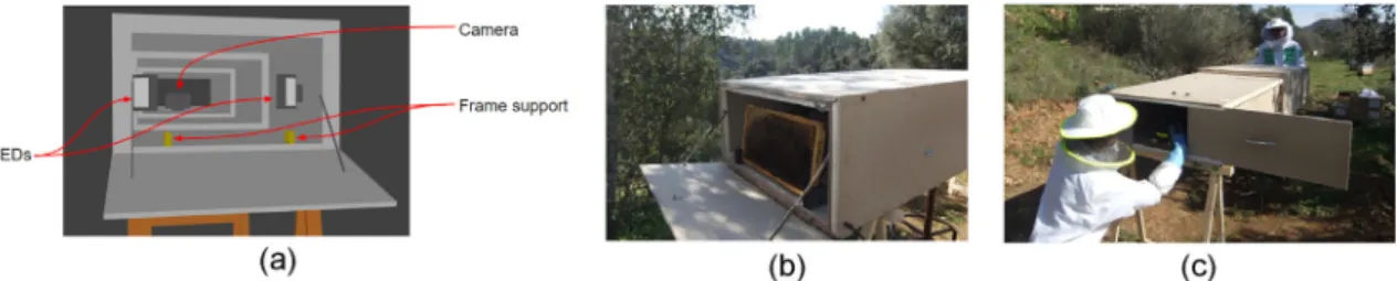
To assure image capture standardization, we developed a wooden tunnel sealed for external light and with optimized dimensions (Fig. 2). This tunnel had a retractable architecture for easy transportation, having a length of 247 cm, when fully opened, and 92 cm, when re-tracted. The comb frame and the camera were placed at the opposite sides of the tunnel. The comb frame was positioned in two holders (Fig. 2b). The holders had an angle of 11° (to make up for to the 9-13° natural inclination of comb cells) for a better image capturing of the interior of the comb cells (see the 3D modelfile inhttps://github.com/ AvsThiago/DeepBee-source). Close to the comb frame (40 cm from the top), there was pair of Light-Emitting Diode (LED) sources, with 7 Watts of power. The LEDs were turned to the walls at 45° to provide homo-geneous light conditions and to avoid shadows during image acquisi-tion. The camera wasfixed with a screw on the opposite side of the tunnel (Fig. 2c). Further details about the tunnel features are shown in Appendix B.
In this study we used a digital camera Nikon D3300, with lens AF-S DX VR Zoom-Nikon ED 55–200 mm F4-5.6G, and the following settings: aperture−10; ISO−100; shutter speed−1/60; autofocus - on;flash -no; compression–JPEG; white balance - on. During image capturing, the tunnel was closed on both sides and the camera was activated by an external trigger. The images captured had a resolution of 24MPixels (6000x4000px). Using these settings, 1,102 comb frames were photo-graphed on both sides making a total of 2,204 images. The image da-taset is available online at https://cloud.ipb.pt/d/ aa29c989ab1944aaa222/?p=/DS-COMB-PT.
3. Scale invariant detection and false detection removal
After obtaining the 2204 images, we searched for a method capable of reliably detecting individual comb cells, a task that precedes cell classification. Below, the different approaches and steps followed in this study are described.
3.1. Circle Hough Transform
Duda and Hart (1972) developed the classical Hough Transform method currently available. This method was originally developed for detecting lines in images. Later on, it was discovered that it could also be used for identifying arbitrary shapes, such as circles and ellipses, even when they were partially occluded.
The Circle Hough Transform (CHT) method uses a voting process to calculate the probability that a set of pixels form a circle. There are several implementations of the method. Herein, we used the im-plementation contained in the OpenCV v.4.0 library (https://github. com/opencv/opencv/releases/tag/4.0.0). The parameters expected by this method are: a grayscale image, size of an internal accumulator that will store intermediate results, minimum distance between two detec-tions centre, threshold to be applied to the internal Canny operator, number of votes that a circle must have in the accumulator to be set as true, minimum circle radius, and maximum circle radius.
3.2. Using CHT to detect cells
Prior to detecting comb cells using CHT, we applied a pre-proces-sing method to normalise illumination, remove noise, and enhance cell edges. The pre-processing pipeline was developed using empirical tests, as follows: (i) extract only the red channel from the image; (ii) apply a Contrast Limited Adaptive Histogram Equalization (CLAHE) (Zuiderveld, 1994) with 8x8 tiles and clip limit of 2.0; (iii) remove the noise keeping the edges by using the bilateral filter (Tomasi & Manduchi, 1998) with diameter 5, sigma colour 50, and sigma space 50.
Having the pre-processing method defined, we started looking for the best parameters combination for CHT. Typically, comb cells have well-behaved diameters and distances and do not overlap. These fea-tures greatly facilitated cell detection by the CHT method. On the other hand,finding a combination of parameters to make CHT capable of detecting uncapped and capped brood and honey cells revealed to be a challenging task to be done by guessing and checking. Therefore, we used a grid search-based algorithm tofind the optimal combination. The best result obtained from our images was: internal accumulator size –3, minimum distance–51, Canny threshold–100, minimum number of votes–25, minimum radius–31, and maximum radius−37.
With this combination of parameters, we were able to successfully detect all different types of cells. However, settingfixed values for the minimum distance, minimum radius and maximum radius makes de-tection less generalist, requiring that images are acquired using a setup like that described above. Therefore, to generalize the method, we developed a scale-invariant detection method, which has two main stages. First, the average cell size and the mean distance between them
Fig. 2.(a) Details of the interior of the tunnel. (b) Tunnel installed in an apiary showing the comb frame placed on holders. (c) Researcher adjusting the camera before shooting.
are sought. Second, all cells are detected using the other parameters discovered by the grid search. The detailed operation involved the following steps (the distances are in pixels):
I. Detect cells with radius belonging to different ranges.In this step, we only considered detections by the CHT method with high levels of confidence (Fig. 3a). Thefixed parameters were: internal accumulator−2, Canny−145, minimum number of votes (con-fidence)–55, and minimum distance−12. We also iterated a loop withiranging from 5 to 50 and step 5. At each iteration, the CHT method was executed with the parametersminRadius=i+ 1 and maxRadius= i + 5. After running this method, a list with the number of detections made for each radiusiwas returned (Fig. 3b). II. Find the most frequent radius.In this step, we selected the most frequent radius from the detections made on the given image with different radiusi.Fig. 3b shows how many radius-based circles were found in the image. Most of the circles were detected with the ra-dius 18, since it is the most frequent cell size for this image. III. Define the minimum distance between two detections.Due to
different cell sizes and imperfections made by honey bees during comb construction, in this step, we had to choose values for the minimum distance parameter smaller than 2 × radius. After ana-lysing the average distance between two cells of numerous frame images of different sizes, we found that usually the minimum dis-tancefits the Eq.(1), whererstands for radius.
= −
minDist r( ) 1.65r 3, (1)
IV. Find the parameters minRadius and maxRadius for a given radius.To deal with the natural variation of comb cell size and with images taken from different distances, in this step, we created a range based on the average cell radius. The range is defined by Eq. (2). = ± ⎧ ⎨ ⎩ > ≤ range r r r if r if r ( ) 0.1 , 0.1 1 1, 0.1 1 , (2)
V.Perform CHT with the obtained parameters.After obtaining the parameters needed, we processed the images again with the CHT method, but this time using the remaining parameters found by the grid search (accumulator size, Canny threshold, minimum number of votes).
Using parameters that accept more detections as true increases the power of detecting different types of cells, even those with fuzzy edges like honey cells (Fig. 3). However, by reducing the threshold for de-tecting all true cells there is a risk of false detections (Fig. 4). To alle-viate this problem, we developed a method based on CNNs, which is described in the ensuing section.
3.3. Removing false detections using semantic segmentation
Semantic image segmentation, also called pixel-level classification, is the task of clustering parts of an image together, which belong to the same object class (Thoma, 2016). We used this technique for detecting comb cells in the image and from this segmentation remove false cells falling outside the comb area (Fig. 4). To that end, we used a CNN encoder-decoder architecture based on U-Net (Ronneberger et al., 2015).
3.3.1. Dataset creation for comb segmentation
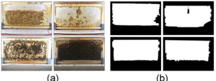
We created the annotations using theQuick Selection Toolfrom the softwareAdobe Photoshop®CS6. To define the classes, we painted white the comb area and black the remaining area. We labelled 61 comb images (Alves et al., 2019), which were selected to represent a high diversity of cell content (e.g. honey, pollen, capped and uncapped brood) and age (the older the comb the darker it gets).Fig. 5illustrates annotations made on those images. The annotations were split in three sets: training (85%); validation (10%), and testing (5%).
Using the strategy proposed inRonneberger et al. (2015), we di-vided the input images and the labels in tiles, as shown inFig. 6. Prior to transforming each image in tiles, a mirrored border with size 184px (top-bottom) by 148px (left-right) was added to create more space for the tiles, and the images were resized to a constant size of 1000x1500px. During tiles extraction, overlaps between tiles were taken into account to reduce border problems in the reassembly phase. Using these processes, we transformed the 61 images into 7137 tiles. Fig. 3.(a) Detection of cells with high confidence by the CHT method. (b) Number of cells detected f radius size.
Fig. 4.Comb cells, with different contents (honey, pollen, capped brood), de-tected by our approach. Dede-tected cells, including false detections outside of the comb, are marked by a green hexagon. The close-up square shows honey cells (on the left half) with fuzzy edges. (For interpretation of the references to colour in thisfigure legend, the reader is referred to the web version of this article.)
3.3.2. Semantic segmentation architecture and training policy
The architecture had a depth of 5 convolutions with 3 × 3filters and layers of maximum pooling with 2 × 2filters and a stride of 2, as proposed byRonneberger et al. (2015). Our modifications to the ori-ginal model, made to obtain the best results in our semantic segmen-tation dataset, were tuned using a trial-error approach and the fol-lowing settings: input image with 128 × 128 resolution, dropout (Srivastava et al., 2014) ranging from 0.1 to 0.3 between the con-volution layers, use of Exponential Linear Units (ELU) activation function (Clevert et al., 2015), and use of 16filters (channels) in the first layer, doubling the amount at each inner level and returning 16 filters in the penultimate layer with the last layer only having two di-mensions. The CNN architecture is shown inFig. 7.
We normalised the input images by dividing each pixel by 255. As we only had two regions to be classified, we used the binary cross-entropy as loss function. The network weights were initialised using the He Normal initialisation (He et al., 2015). For the output layer, we chose a sigmoid function, so we could easily transform the output in a binary image applying a threshold, where values < 0.5 became zero and the remaining became one. The best training was carried out using the Adam optimiser (Kingma & Ba, 2014) with parametersβ1 = 0.9 andβ2 = 0.999. The Learning Rate (LR) was 10−3, which was pre-served during 50 epochs. Due to the Early Stopping method used here, the training may last less than 50 epochs. This method can halt the training if a chosen metric does not improve after a pre-defined number of epochs (6, in this study). The architecture was built using the fra-mework Keras 2.1.4 with TensorFlow 1.4 as backend. The confi gura-tions of the computer used for training were two GPUs: NVIDIA Ge-Force GTX 1080Ti and NVIDIA GeGe-Force GTX 1070; RAM: 16 GB; CPU: Intel® Core™ i7-7700 K CPU @ 4.20 GHz × 8; operating system: Ubuntu 17.10. All tests were performed in this computer.
3.3.3. Post-processing of comb segmentation
A post-processing step was undertaken so that the segmented image could be used to minimize false detections. To have a binary output
after the CNN computation, we applied a threshold of 0.5 and the tiles were reassembled. Subsequently, we found the largest contour using an OpenCV method forfinding contours and draw itfilled using a method to draw polygons (Fig. 8). Filtering using the largest contour helped removing false segmentations inside and outside the comb, as shown in Section 5.1.2.
3.4. Semantic segmentation experiments
In thefirst experiment, we assessed the quality of detections on an independent set of 10 comb images, which were downloaded from the Internet. This set was submitted to the scale-invariant cell detection algorithm and the false detections removal method.
In the second experiment, we measured the cells detection rate of our algorithm and compared with that proposed byLiew et al. (2010). Following the methodology ofLiew et al. (2010), we selected 10 images from our dataset to be analysed by our detection algorithm. Subse-quently, we evaluated manually the false positive (FP) and false nega-tive (FN) detections. From these annotations, we collected the following metrics: number of cells identified by humans; number of cells detected by the algorithm; true positive (TP) detections; true cells detected correctly; FP detections on inexistent cells; and FN cells undetected by the algorithm. Finally, as inLiew et al. (2010), we calculated for each image the cells detection rate using Eq.(3). This metric is based on the total number of cells automatically detected, excluding the falsely identified cells, divided by the manual count.
= − ×
Cell Detection Rate Detection Count FP
Manual Count 100% (3)
4. Cells classification
The cell classification was carried out using CNNs. This supervised approach gained momentum after the release of Krizhevsky et al. (2012)work. At the time, this work was considered the state-of-the-art in the ImageNet Large Scale Visual Recognition Challenge, where the goal was to accurately classify more than a million images into 1000 distinct classes. After this seminal work, important advances have been made in CNN architectures, with major consequential breakthroughs in variousfields of study such as agriculture (Kamilaris & Prenafeta-Boldú, 2018). A key feature for training a CNN architecture is the massive amount of data needed. Following, we show how we gathered the cells images for our dataset.
4.1. Dataset gathering for cells classification
The dataset created for classification should contain cells re-presenting all different classes in different comb images. In this study, Fig. 5.Samples from the dataset created for semantic segmentation: (a) original
image; (b) label.
the annotations were made by an experienced beekeeper, assuring the high quality required for developing the models. A piece of software was developed to facilitate the beekeeper’s work. The software allowed choosing a label corresponding to each class (nectar, honey, pollen, egg, larva, capped brood, and other) and, at the same time, pointing the centre of the cells, adjusting the contrast, brightness and gamma of the images. A total of 71,915 cells were annotated on 1202 comb images, with an average of 25 cells per image. The number of annotations by class is shown inFig. 9.
We divided the annotations in three sets for the training as follows: 80% of the original dataset for training, 20% of the training set for validation, and 20% of the original dataset for testing. Then, we se-lected 15 additional comb images and annotated all the cells. We made a total of 39,533 new annotations and added them to the test set. 4.2. Transfer learning for cells classification
Using the transfer learning technique, it is possible to transfer the weights of feature extraction layers (e.g. convolutions) from a trained
model over a dataset to another model that will be trained in a new dataset (Oquab et al., 2014). Because the new model received kernels already trained to recognise generic features, like lines and curves, it will be easier for the model to generalise a new dataset being un-necessary to learn thefilters from scratch. We made a sanity check and trained an architecture in our dataset with and without the transfer learning before applying this approach to the next experiments. In this experiment, we used the same policy in both trainings. We transferred the weights from a pre-trained model on the ImageNet dataset (Deng et al., 2009). We used the architecture InceptionV3 (Szegedy et al., 2015) and, as shown inFig. 10, the model converged faster, in a lower number of epochs and with a higher accuracy with the transfer learning than with training from scratch.
4.3. Finding the best region of interest (ROI) size to crop the cells Before we defined the CNN architecture for the classifier, we needed tofind at which window size around the cells the image should be Fig. 7.CNN architecture based on U-Net to handle comb segmentation.
Fig. 8.Process developed to reduce the number of false segmented areas.
Fig. 9.Number of annotations per class.
Fig. 10.Comparison between models trained in our dataset from scratch and using pre-trained weights from ImageNet.
cropped. If we had cropped only the interior of the cells, our classifier could have had difficulty in distinguishing between capped brood and honey cells, as these classes typically exhibit a similar texture (Fig. 11). To select the best input size, we created and tested 16 datasets, all of them with the same annotations but with different ROI size. We defined each dataset with 10% of the annotations from the main dataset. The sizes (pixels) of the squared crops were 40, 50, 60, 80, 100, 120, 140, 160, 180, 200, 220, 240, 280, 298, 400 and 500.
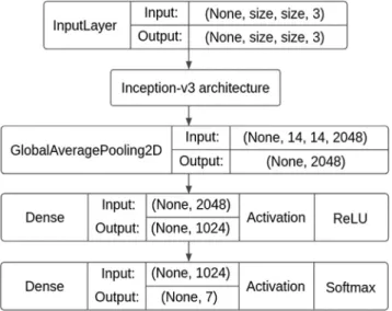
The training framework for the tests was the Keras version 2.2 and the InceptionV3 architecture (Szegedy et al., 2015). For the feature extraction layers, we used weights pre-trained on the ImageNet dataset using the transfer learning technique. The architecture and trained weights were provided by Keras library. This architecture does not allow inputs lower than 139 × 139px. Image datasets lower than 139 × 139px were resized to the minimum input size. We added three layers at the end of the architecture to create the specific learning on the classifier. Thefirst one was aflattening layer applied to the network output. Afterwards, we included two Dense layers (fully-connected) with the last one having 7 neurons and a Softmax activation function to represent our classes in a linear probabilistic domain. Details about the architecture are shown inFig. 12.
The classifiers were compiled using the Categorical Cross Entropy loss function. We chose Adam with default parametersβ1 = 0.9 and β2 = 0.999 as the optimiser. The training started with the LR at 10−3 and using the technique Reduce Learning Rate on Plateau (He et al., 2015a). We defined that the LR would be halved after 3 epochs without improvement in the Loss metric, being the minimum value 10−6. We established 50 for the maximum number of epochs. Again, we used the Early Stopping technique with the maximum number of epochs, without improvement, set at 5. We saved the model with the lowest validation Loss in each dataset. The best results were provided by a window size of 224 × 224px. We opted for 224 × 224px rather than
220 × 220px, for the reasons pointed out inSection 5.2.1.
4.4. Tests with different CNN architectures
After obtaining the best window size, as described previously, we trained different CNN architectures with the input size 224 × 224px to identify which one produced the best results on our dataset. We trained 13 distinct architectures selected by their superior performance in image classification competitions in the past years. These architectures included DenseNet 121, DenseNet 169, DenseNet201 (Huang et al., 2016), InceptionResNetV2 (Szegedy et al., 2016), InceptionV3 (Szegedy et al., 2015), MobileNet (Howard et al., 2017), MobileNetV2 (Sandler et al., 2018), NasNet; NasNetMobile (Zoph et al., 2017), ResNet50 (He et al., 2015a), VGG 16, VGG 19 (Simonyan & Zisserman, 2014), and Xception.
Each architecture was trained using all training and validation images from the core dataset. The images were extracted with the cell centralised 224 × 224px. Before starting training each model, we made some modification in the CNN architectures. We added a set of fully-connected layers, as shown inFig. 12. Prior to processing by the model, the images were normalised by subtracting the ImageNet Mean Image (103.939, 116.779, 123.68). The weights were transferred from pre-vious ImageNet trainings. The training was performed with batches of 40 images. We defined the initial LR at 10−3 and used the Early Stopping and Reduce LR on Plateau, as inSection 4.3. For comparing the model, we extracted some information and metrics, including total architecture parameters (weights), time to process an image batch, training time, accuracy, loss, precision, recall and F1-score.
4.5. Data augmentation
It is not always possible to obtain large datasets for training CNNs, either due to difficulties in gathering images with the object or in af-fording human resources to annotate the datasets. One way to enlarge the working dataset is through the Data Augmentation (DA) technique (Krizhevsky et al., 2012). Using DA, it is possible to create virtual ex-amples from a set of images. Different transformations with random values are applied to these images and new ones are generated. Ex-amples of transformations include changes in brightness, contrast, translates, rotations, zoom, and perspective.
Based on the models with the best metrics discovered in the ex-periment described inSection 4.3, we made a new training with addi-tional data. We generated the new images using DA. Flips, brightness changes, rotations, shift, and zoom were applied in the newly created images. As a result, we generated a dataset of 250,000 images evenly spread across the 7 different classes. These images were used in the training set. Validation and test sets were kept with the original images. We compared the resultant models using the metrics described in Section 4.3.Fig. 13shows several examples generated using DA. Fig. 11.Comparison between (a) honey and (b) capped brood classes. In
ad-dition to the cells interior (a1, b1), the cells neighbourhood (a2, b2) was taken into consideration to better define the two classes.
5. Results and discussion
5.1. Cells detection and false detection removal 5.1.1. Cells detection
In thefirst cell detection experiment, we assessed the performance of the developed algorithm in a set of independent images downloaded from the internet. After selecting images that were captured under a wide range of conditions, we generated the results, some of which are illustrated inFig. 14.
The algorithm successfully detected most comb cells of the selected images (Fig. 14). These images represented a wide range of hive frame type, cell size, cell content (e.g. honey, capped and uncapped brood), and even varying illumination, texture and resolution, suggesting that the algorithm developed in this study is robust.
5.1.2. False detection removal
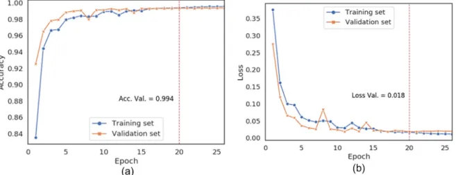
The training of the CNN for segmentation was carried out with 23 epochs in 3.45 min on the computational architecture referred in Section 3.3.Fig. 15shows the evolution of accuracy and loss metrics in the training and validation sets along the epochs. The model loss im-proved quickly before the 10th epoch; after that, only small improve-ments were achieved, even with the constant learning rate.
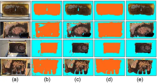
Using a CNN to segment the comb proved to be a robust solution, as it delivered great results even on the independent set of images.Fig. 16 shows some examples of segmentations performed in the independent and in our image sets. The downside is that CNN may have difficulty in segmenting when the comb cells have not yet been developed (there is only wax foundation) and when honey cells are very bright. The deci-sion of selecting only the largest polygon and fill it to create a mask contributed to removing false segmentations inside and outside the comb area, as illustrated inFig. 16. This approach has a poorer per-formance on combs that are broken (see bottom image ofFig. 16a) or
have objects on front (see the thermohygro sensor on the top image of Fig. 16a), for example. However, these comb defects are unusual. 5.1.3. Comparative analysis
To measure the quality of the detections using the segmentation, we performed several tests, similar to those ofLiew et al. (2010), on 10 selected images. The results of these tests are shown inTable 1. False cell-related or noise-related detections were negligible in our tests, as found byLiew et al. (2010). A factor that had a negative impact on the results ofLiew et al. (2010)work was the low contrast in some cells. As detailed onSection 3.2, we dealt with this problem by applying the CLAHEfilter to our images before detecting the cells.
As inLiew et al. (2010), we calculated the cell detection rate for each image using Eq.(3). The resulting detection rates varied between 97.35% and 99.9%, with an average of 98.7% (Table 2). These rates were substantially higher than those reported byLiew et al. (2010). However, the method ofLiew et al. (2010)produced a lower number of FP (5.1) than our method (22.5). This difference can be explained by the fact thatLiew et al. (2010)used more stringent parameters for CHT, allowing only detections with a high level of confidence. On the other hand, when we examined the number of FN, our approach produced substantially better results (38.2 compared with 274.7; Table 2). Overall, the method developed in this study revealed to be well ba-lanced regarding FP and FN and these metrics had a small impact on cell detection rate (98.7%).
5.2. Cells classification
5.2.1. Finding the optimal input image size
After training 16 different classification models, we obtained a plot relating ROI size with cell classification accuracy (Fig. 17). The trending line shows a steady increase in the accuracy as the ROI size increases up to 300px; after that point the quality decreases. Fig. 14.Cells detected with (a) radius 18 (leahybeekeeping.com), (b) radius 8 (mudsongs.org), and (c) radius 48 (beekeepercenter.com).
Fig. 15.Evolution of (a) accuracy and (b) loss during training of the comb semantic segmentation model. The vertical dashed line over the 20th epoch represents the best calculated results (lowest loss).
Accordingly, input images with sizes between 200px and 300px should be preferred as they tend to produce better results.
We chose 224 × 224px as the default input size for all the following tests. We based this choice on the computational cost. Additionally, although the best result in the test set was the one trained with 220 × 220px images, it was not possible to use this input size because architectures like MobileNetV2 only had pre-trained weights in the ImageNet dataset for sizes 128, 160, 192, or 224px (https://bit.ly/ 2DhnLRb). To avoid the hassle of comparing models trained with varying input sizes, we opted for using only 224 × 224px across all tests.
5.2.2. Comparing different CNN architectures
During the training of different architectures with the 224 × 224px input size, we faced some difficulties. We noticed that models VGG 16 and 19 were unable to converge over the used dataset (10% of our original dataset), even after trying different LRs, loss functions and optimisers. Therefore, we decided to remove these two models from the tests. Another model that caused problems during the training stage was NasNet (Large). This model suffers from a known bug (seehttps://
github.com/keras-team/keras/issues/8711#issuecomment-354585187) and there are bypasses for it, but we decided to discard it due to the large amount of time required for retraining.
Table 3presents some metrics for the computational performance of 11 models. The MobileNet model produced the best results regarding the number of epochs required for reaching convergence and the average time per epoch. MobileNet weights number was also among the lowest, only behind of its second version.
To better understand the performance of the models, we also Fig. 16.(a) Original image, (b) segmentation mask provided by the CNN without post-processing, (c) segmentation mask applied to the original image, (d) largest contour used as a mask, (e) largest contour applied to the original image.
Table 1
Comparison between cells detected automatically and cells detected automatically and manually corrected.
Image name Manual count Automatic count TP TP (%) FP FP (%) FN FN (%) CDR (%) DSC_1940.JPG 3024 2949 2944 97.35 5 0.17 80 2.65 97.35 DSC_1992.JPG 2795 2742 2735 97.85 7 0.26 60 2.15 97.85 DSC_2832.JPG 2869 2833 2794 97.39 39 1.38 75 2.61 97.39 DSC_2839.JPG 3082 3062 3041 98.67 21 0.69 41 1.33 98.67 DSC_2864.JPG 2961 2982 2948 99.56 34 1.14 13 0.44 99.56 DSC_2951.JPG 2910 2889 2857 98.18 32 1.11 53 1.82 98.18 DSC_2443.JPG 2077 2088 2075 99.90 13 0.62 2 0.10 99.90 DSC_3475.JPG 2875 2876 2852 99.20 24 0.83 23 0.80 99.20 DSC_4326.JPG 3061 3092 3054 99.77 38 1.23 7 0.23 99.77 DSC_4496.JPG 3072 3056 3044 99.09 12 0.39 28 0.91 99.09
CDR–Cell detection rate; FP False Positive; FN False Negative; TP True Positive. Table 2
Performance metrics for the detection methods developed in this study and in Liew et al. (2010).
Method Min FP Max FP Avg FP Min FN Max FN Avg FN Avg CDR (%) Liew et al. 1 11 5.1 139 530 274.7 82.5 Ours 5 39 22.5 2 80 38.2 98.7
CDR–Cell detection rate; FP False Positive; FN False Negative.
Fig. 17.Testing accuracy according to the ROI size. The dashed green line represents the trend. (For interpretation of the references to colour in thisfigure legend, the reader is referred to the web version of this article.)
analysed the loading time and the time to predict a batch of 100 images (Fig. 18). These additional analyses were important to predict how the models behave, regarding time-efficiency performance, when used after training. Once again, MobileNet showed the best performance when compared with the other models. Even though MobileNet had fewer parameters than most models (Table 3), it was still the fast one to be loaded into memory.
To evaluate the functional quality of the classifications, we first compared the loss and accuracy of each model in their best epochs (Table 4). The model ResNet50 showed a higher capacity to predict training examples, but performed worse on the other sets, probably due to overfitting. DenseNet201 exhibited the best accuracy in the valida-tion and test sets, but its predicvalida-tions were made with less confidence when compared with MobileNet, which had the lowest loss score in the validation and test sets.
Sometimes accuracy can be biased by the majority class. To better understand this bias, we calculated precision, recall and F1-score for each model on the test set. As shown inFig. 19, InceptionResNetV2 had the best performance, exhibiting a good balance between accuracy and recall. DenseNet201 had the best accuracy in the test set, yet it was positioned in seventh place for the F1-Score metric. This result suggests that DenseNet201suffered by overfitting and favoured the majority class.
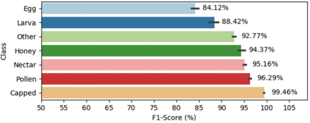
In the per class analysis, we assessed how well each model classified the comb cell contents into the seven established classes. As shown in Fig. 20, the egg class exhibited the highest proportion of incorrect predictions (15.88%) whereas the capped brood class was very close to 100% correct predictions, based on F1-Score. This is an expected result as capped brood cells are simpler to classify due to their striking visual differences when compared with the remaining classes (Fig. 9). The egg class may have suffered from being the minority class. Eggs are small objects placed at the bottom of the cells and are easily confused with light reflections. Moreover, establishing thresholds for egg/empty and egg/young larva cells is a challenging endeavour. This issue will be further addressed inSection 5.2.5.
models, with an F1-score over 94%.
Given that InceptionResNetV2 and MobileNet exhibited the highest score after training with DA, we decided to employ again the F1-Score to compare the resources required to train and use these models for each class. As shown inFig. 22, while the difference between the two models in the quality of results per class is modest, MobileNet re-vealed to be superior for computational resources across all perfor-mance metrics. The superior perforperfor-mance of MobileNet can be attrib-uted to the lower number of trainable parameters. Hence, the model complexity is reduced, regarding the number of training examples, counteracting overfitting.
5.2.4. Comparison with methods from the literature
Here we compared our method with those reported in the literature, although this endeavor may not always be fair for three main reasons: (i) we classified a wider array of cell types, (ii) we do not have the same dataset, and (iii) some works employed different classifiers.
Cornelissen et al. (2009)compared their semi-automatic method of counting capped brood cells in comb images with the Liebefeld method. While annotations with the Liebefeld method took 26 s per frame, the semi-automatic approach took 19 s for image capturing plus 30 s for image processing. This semi-automatic method consists of manual segmentation of the capped brood area followed by automatic count of cell number.
Fig. 23presents the time distribution required by each phase of our cell detection and classification approach. The results were obtained from processing all 61 images of the segmentation dataset using the scaled invariant detection algorithm and the MobileNet model trained with DA. The time required to fully process an image varied between ~4 and ~16 s, with an average of 9.07 s. Considering only the average value, the time to photograph a frame and process the image was 28.07 s using our setup, which was about 2 s slower than the Liebefeld method for capped brood cells.
Cornelissen et al. (2009)reported a correlation of 99.37% between the actual and the predicted number of cells, which was substantially higher than the 90.85% obtained with the Liebefeld method. Our ap-proach correctly detected 98.7% of the cells. Using CNNs, we obtained an F1-Score of 99.47% and 99.77% for the capped brood class with the MobileNet-DA model and the InceptionResNetV2-DA model, respec-tively.
Our approach of cell detection and classification overcomes some important challenges pointed out byColin et al. (2018). By using a CNN
MobileNet 11 211.58 4,285,639 MobileNetV2 31 235.98 3,576,903 NASNet 28 2332.04 89,053,785 NasNetMobile 21 393.81 5,359,259 ResNet50 25 343.45 25,693,063 Xception 14 503.87 22,966,831
model, we were able to distinguish capped honey from capped brood. Furthermore, by using a grid search forfinding good parameters for the CHT and the semantic segmentation, we dismissed the user interaction for detecting the cells.
Rodrigues et al. (2016)obtained a precision of 99.04% and a recall of 97.2% for the capped brood class. In our analyses, using the Mobi-leNet DA model, we were able to improve those metrics up to 99.47% and 99.41%, respectively.
Wang and Brewer (2013)reported a 97.4% hit rate with the Hon-eybeeComplete commercial software developed for counting capped brood cells. This value increased to 99.5% when the search area was delineated by the user in the comb image. Herein, the MobileNet DA architecture produced a value for the capped brood class very close (99.47%) to that obtained by the HoneybeeComplete software, but without human assistance.
The commercial softwareHiveAnalyzer(Höferlin et al. 2013), which is able to classify detected comb cells into seven classes, achieved Table 4
Comparison of loss and accuracy between models in different sets.
Model name Loss train Acc train Loss val Acc val Loss test Acc test DenseNet121 0.00818 99.75% 0.05213 98.56% 0.25716 93.71% DenseNet169 0.00159 99.95% 0.06365 98.58% 0.37087 93.12% DenseNet201 0.00115 99.97% 0.05990 98.66% 0.31397 93.94% InceptionResNetV2 0.00425 99.89% 0.05986 98.55% 0.29882 93.45% InceptionV3 0.00415 99.90% 0.05594 98.58% 0.27237 93.47% MobileNet 0.01563 99.57% 0.05106 98.48% 0.23944 93.31% MobileNetV2 0.00942 99.69% 0.06468 98.57% 0.37828 93.02% NasNetMobile 0.00162 99.94% 0.07417 98.56% 0.37836 93.79% ResNet50 0.00033 99.99% 0.08845 98.44% 0.39329 92.99% Xception 0.01173 99.73% 0.06574 98.54% 0.36011 92.70%
Fig. 19.Precision, recall and F1-score calculated using different models. The models are sorted by F1-Score.
Fig. 20.Average F1-score per class.
94.3% accuracy on cells that were classified with high confidence (78% of 20,000 analysed cells). In this study, we achieved 94.31% accuracy (very close to the 94.3% F1-Score value) using the MobileNet model DA on 100% of the test set (53,914 analysed cells). When we selected predictions with confidence > 99.6% (corresponding to 42,410 cells and 78.66% of the dataset), we obtained 99.35% accuracy, a sub-stantially higher rate than that ofHöferlin et al. (2013).
5.2.5. Further analyses on datasets creation and cells classification The task of correctly classifying all the cells in a comb image is not trivial because of the wide range of colours, shapes, and textures of cell contents and wax types typically found in a hive. While working with the datasets, we realized that comb classification is further challenging due to the impact of some factors on the results quality. One such factor was related with cell contents. Cells with multiple contents (e.g. pollen and egg) or cells with contents in a transition stage, such as from larva to pupa (capped cell) or from egg to larva, revealed to be problematic (Fig. 24).
The co-occurrence of different cell contents makes evaluation of the classifier less precise, as there may be cases where it hits one of the classes but the alternative class has been defined as the ground truth of the image. This problem has been handled in competitions of image classification using Top-n accuracy (Krizhevsky et al., 2012). With this methodology, the model earns credit for correctly classifying the image in its Top N guesses. We evaluated our model using Top-2 accuracy, which corrected the cell content if the correct class was between the two more likely predictions. By reprocessing the test set with the Top-2 accuracy method, the quality of our results improved 5% on average (Fig. 25).
Another factor affecting the quality of the results is related with the positions most annotated by the beekeeper. We noticed that there was an inverse relationship between the areas most frequently labelled by the beekeeper and the areas where most incorrect predictions occur. Due to the camera-optical behaviour, cells in different regions of the comb may display different areas of their interior, as illustrated in Fig. 26. This effect could impact cell classification if certain regions of the images were favoured during the annotation process. One way to alleviate this problem is to place the camera far from the frame and use a uniform light to diminish shadows during image capture.
To test this effect, we assessed the distribution of the annotations across comb regions. To that end, using the annotations of the main dataset, we generated a heatmap plot displaying the areas of the comb that were preferentially annotated. As shown inFig. 27a, annotations were more concentrated in the upper left area of the comb, suggesting that models trained in this dataset would have a better classifying performance in that region. Next, we predicted all cells that were Fig. 22.Comparison between the models MobileNet and InceptionResNetV2 using (a) F1-score by class and (b) resources by DA model.
Fig. 23.Time distribution to detect and classify all cells in a comb image.
Fig. 24.(a) Transition from egg to young larva; (b) transition from old larva to moulting, when cells will be capped; (c) transition from nectar to honey, when cells will be capped; (d) central cell containing pollen and an egg.
homogeneously annotated in the test set and generated a new heatmap showing the location of most of the wrong predictions (Fig. 27b).
According to both heatmaps, incorrect predictions occurred mostly in the lower-right regions of the comb, and this pattern was inversely related with the regions where more annotations were made. This spatial pattern of annotations becomes more striking in the heatmaps generated by class (Fig. 28). Altogether, these results suggest that training a good classifier requires not only a large number of annota-tions but also a homogeneous distribution across the comb. Only then the annotations can inform the model, during the training, about the different angles that cells can present and help in the generalisation.
5.3. DeepBee© software
With all the methods developed and presented herein we built a software that we namedDeepBee© (Fig. 29). This software allows the user to automatically process a batch of comb images. After processing the images, the user can view the results, change prediction labels, if needed, add and remove new detections, and export all results for further analysis into a spreadsheet like excel. DeepBee© is freely available athttps://avsthiago.github.io/DeepBee/.
Fig. 26.Different cells interior captured in dif-ferent regions due to lens effects (a) Upper left cell; (b) Upper right cell; (c) Central cell; (d) Lower left cell; (e) Lower right cell.
Fig. 27.Distribution of annotations in the comb. Comparison between (a) most annotated areas and (b) with more errors.
Fig. 28.Comparison among the most annotated areas and with more errors by class.
demonstrated that by applying the semantic segmentation technique it is possible to remove false detections that may occur on the back-ground. Although we obtained a cell detection rate of 98.7%, we be-lieve that the false positive rate may decrease by training the semantic segmentation model with an input larger than 128 × 128px.
After we trained over thirty CNN models with different training techniques, such as transfer learning and data augmentation, and comparing them using different perspectives, we recommend MobileNet. While InceptionResNetV2 showed the best results in our dataset, the time performance of MobileNet was superior, due to 93% fewer weights. Using MobileNet, we achieved 94.3% of correctness with the metric F1-score weighted over the seven classes. We believe this rate can be further improved using annotations more evenly spread across comb images. The model learned some human biases during the training and became better in classifying cells in some comb regions in detriment of others.
To the best of our knowledge, the cell detection rate and the cell classification accuracy of our model outperformed similar works re-ported in the literature. Future work will focus on development of a service that enables users to process images remotely. Using this web service, even devices with less power, such as smartphones, will be able to run DeepBee©. To deal with low resolution images from smart-phones, we intend to create one composition of many images taken near to the comb frame. With this web service, it will be possible to use detection corrections of the users to improve future results by retraining the classifier.
Declaration of Competing Interest
The authors declare that they have no known competingfinancial interests or personal relationships that could have appeared to influ-ence the work reported in this paper.
Acknowledgements
This research was developed in the framework of the project “BeeHope - Honeybee conservation centers in Western Europe: an in-novative strategy using sustainable beekeeping to reduce honeybee decline”, funded through the 2013-2014 BiodivERsA/FACCE-JPI Joint call for research proposals, with the national funders FCT (Portugal), CNRS (France), and MEC (Spain).
Appendix A. Supplementary material
Supplementary data to this article can be found online athttps:// doi.org/10.1016/j.compag.2020.105244.
References
Alves, T., Pinto, M.A., Candido Junior, A., De Paula Filho, P.L., Rodrigues, P.J.S., Ventura, P., Neves, C., 2019. DS-COMB-SEG-BEEHOPE, Mendeley Data, v1 http://dx.doi.org/ 10.17632/db35fj73x5.1.
Clevert, D.-A., Unterthiner, T., Hochreiter, S., 2015. Fast and Accurate Deep Network Learning by Exponential Linear Units (ELUs). CoRR, abs/1511.0. Retrieved from http://arxiv.org/abs/1511.07289.
Colin, T., Bruce, J., Meikle, W.G., Barron, A.B., 2018. The development of honey bee colonies assessed using a new semi-automated brood counting method: combcount. PLoS ONE 13 (10), 1–14.https://doi.org/10.1371/journal.pone.0205816.
Cornelissen, B., Schmid, S., Henning, J., Der, J. Van, 2009. Estimating colony size using
on assessing the health status of managed honeybee colonies (HEALTHY- B): a toolbox to facilitate harmonised data collection. EFSA Journal 2016;14(10):4578, 241 pp. doi: 10.2903/j.efsa.2016.4578.
Emsen, B., 2006. Semi-automated measuring capped brood areas of honey bee colonies. J. Anim. Veterin. Adv.
He, K., Zhang, X., Ren, S., Sun, J., 2015a. Deep residual learning for image recognition. CoRR, abs/1512.03385. Retrieved from http://arxiv.org/abs/1512.03385. He, K., Zhang, X., Ren, S., Sun, J., 2015b. Delving deep into rectifiers: surpassing
human-level performance on ImageNet classification. CoRR, abs/1502.0. Retrieved from http://arxiv.org/abs/1502.01852.
Höferlin, B., Höferlin, M., Kleinhenz, M., Bargen, H., 2013. Automatic analysis of apis mellifera comb photos and brood development. In: Association of Institutes for Bee Research Report of the 60 th Seminar in Würzburg (Vol. 44, p. 19). Apidologie. Retrieved fromhttps://www.springer.com/cda/content/document/cda_ downloaddocument/AGIB-Abstracts 2013_Final.pdf?SGWID=0-0-45-1417002-p174076256.
Howard, A.G., Zhu, M., Chen, B., Kalenichenko, D., Wang, W., Weyand, T., et al., 2017. MobileNets: Efficient Convolutional Neural Networks for Mobile Vision Applications. https://doi.org/10.1016/S1507-1367(10)60022-3.
Huang, G., Liu, Z., Weinberger, K.Q., 2016. Densely connected convolutional networks. CoRR, abs/1608.06993. Retrieved from http://arxiv.org/abs/1608.06993.
Kamilaris, A., Prenafeta-Boldú, F.X., 2018. Deep learning in agriculture: a survey. Comput. Electron. Agric. 147, 70–90 https://doi.org/https://doi.org/10.1016/ j.compag.2018.02.016.
Kingma, D. P., Ba, J., 2014. Adam: {A} Method for Stochastic Optimization. CoRR, abs/ 1412.6. Retrieved from http://arxiv.org/abs/1412.6980.
Krizhevsky, A., Sutskever, I., Hinton, G.E., 2012. ImageNet classification with deep convolutional neural networks. In: Pereira, F., Burges, C.J.C., Bottou, L., Weinberger, K.Q. (Eds.), Advances in Neural Information Processing Systems 25 (pp. 1097–1105). Curran Associates, Inc. Retrieved from http://papers.nips.cc/paper/4824-imagenet-classification-with-deep-convolutional-neural-networks.pdf.
Liew, L.H., Lee, B.Y., Chan, M., 2010. Cell detection for bee comb images using Circular hough transformation. CSSR 2010 - 2010 International Conference on Science and Social Research, (Cssr), 191–195. https://doi.org/10.1109/CSSR.2010.5773764. Oquab, M., Bottou, L., Laptev, I., Sivic, J., 2014. Learning and transferring mid-level
image representations using convolutional neural networks. In: 2014 IEEE Conference on Computer Vision and Pattern Recognition, pp. 1717–1724. https:// doi.org/10.1109/CVPR.2014.222.
Rodrigues, P., Neves, C., Pinto, M.A., 2016. Geometric contrast feature for automatic visual counting of honey bee brood capped cells. EURBEE 2016: 7th European Conference of Apidology, 7. Retrieved from http://hdl.handle.net/10198/17318. Ronneberger, O., Fischer, P., Brox, T., 2015. U-Net: convolutional networks for
biome-dical image segmentation. CoRR, abs/1505.0. Retrieved from http://arxiv.org/abs/ 1505.04597.
Sandler, M., Howard, A.G., Zhu, M., Zhmoginov, A., Chen, L.-C., 2018. Inverted residuals and linear bottlenecks: mobile networks for classification, detection and segmenta-tion. CoRR, abs/1801.04381. Retrieved from http://arxiv.org/abs/1801.04381. Simonyan, K., Zisserman, A., 2014. Very deep convolutional networks for large-scale
image recognition, CoRR, abs/1409.1556. Retrieved from http://arxiv.org/abs/ 1409.1556.
Srivastava, N., Hinton, G., Krizhevsky, A., Sutskever, I., Salakhutdinov, R., 2014. Dropout: a simple way to prevent neural networks from overfitting. J. Mach. Learn. Res. 15, 1929–1958 http://jmlr.org/papers/v15/srivastava14a.html.
Szegedy, C., Ioffe, S., Vanhoucke, V., 2016. Inception-v4, Inception-ResNet and the im-pact of residual connections on learning. CoRR, abs/1602.07261. Retrieved from http://arxiv.org/abs/1602.07261.
Szegedy, C., Vanhoucke, V., Ioffe, S., Shlens, J., Wojna, Z., 2015. Rethinking the inception architecture for computer vision. CoRR, abs/1512.00567. Retrieved from http:// arxiv.org/abs/1512.00567.
Thoma, M., 2016. A survey of semantic segmentation. CoRR, abs/1602.0. Retrieved from http://arxiv.org/abs/1602.06541.
Tomasi, C., Manduchi, R., 1998. Bilateral Filtering for Gray and Color Images. In: Proceedings of the Sixth International Conference on Computer Vision (p. 839). Washington, DC, USA: IEEE Computer Society. Retrieved from http://dl.acm.org/ citation.cfm?id=938978.939190.
Wang, M., Brewer, L., 2013. New computer methods for honeybee colony assessments. In: 8th SETAC Europe Special Science Symposium. Retrieved fromhttp://sesss08.setac. eu/embed/sesss08/Larry_Brewer_-_New_Computer_Methods_for_Honeybee_Colony_ Assessments.pdf.
Yoshiyama, M., Kimura, K., Saitoh, K., Iwata, H., 2011. Measuring colony development in honey bees by simple digital image analysis. J. Apic. Res. 50 (2), 170–172.https:// doi.org/10.3896/IBRA.1.50.2.10.
Zoph, B., Vasudevan, V., Shlens, J., Le, Q.V., 2017. Learning transferable architectures for scalable image recognition. CoRR, abs/1707.07012. Retrieved from http://arxiv.org/ abs/1707.07012.
Zuiderveld, K., 1994. Graphics Gems IV. In: Heckbert, P.S. (Ed.) (pp. 474–485). San Diego, CA, USA: Academic Press Professional, Inc. Retrieved from http://dl.acm.org/ citation.cfm?id=180895.180940.