Quantile regression with L1-regularization and Gaussian kernels

Quantile Regression with

`

₁

−

regularization and

Gaussian Kernels

†

Lei Shi

, Xiaolin Huang

, Zheng Tian

and Johan A.K. Suykens

1

_{Department of Electrical Engineering, KU Leuven,}

ESAT-SCD-SISTA, B-3001 Leuven, Belgium

2

_{Shanghai Key Laboratory for Contemporary Applied Mathematics,}

School of Mathematical Sciences, Fudan University

Shanghai 200433, P. R. China

Abstract

The quantile regression problem is considered by learning schemes based on

`1−regularization and Gaussian kernels. The purpose of this paper is to present an

concentration estimates for the algorithms. Our analysis shows that the convergence behavior of `1−quantile regression with Gaussian kernels is almost the same as

that of the RKHS-based learning schemes. Furthermore, the previous analysis for kernel-based quantile regression usually requires that the output sample values are uniformly bounded, which excludes the common case with Gaussian noise. Our error analysis presented in this paper can give satisfactory convergence rates even for unbounded sampling processes. Besides, numerical experiments are given which support the theoretical results.

Key words and phrases. Learning theory, Quantile regression, `1-regularization,

Gaussian kernels, Unbounded sampling processes, Concentration estimate for error anal-ysis

AMS Subject Classification Numbers: 68T05, 62J02

†The corresponding author is Lei Shi. Email addresses: [email protected] (L. Shi), [email protected] (X. Huang), [email protected] (Z. Tian) and [email protected] (J. Suykens).

1

Introduction

In this paper, under the framework of learning theory, we study `1−regularized quantile

regression with Gaussian kernels. Let X be a compact subset of Rn _{and Y ⊂ R, the}

goal of quantile regression is to estimate the conditional quantile of a Borel probability measure ρ on Z :=X ×Y. Denote by ρ(·|x) the conditional distribution ofρ atx ∈X, the conditional τ−quantile is a set-valued function defined by

Fτ

ρ(x) ={t∈R:ρ((−∞, t]|x)≥τ and ρ([t,∞)|x)≥1−τ}, x∈X, (1.1)

where τ ∈ (0,1) is a fixed constant specifying the desired quantile level. We suppose that Fτ

ρ(x) consists of singletons, i.e. there exists an fρτ :X → R, called theconditional

τ−quantile function, such that Fτ

ρ(x) = {fρτ(x)} for x ∈ X. In the setting of learning

theory, the distribution ρ is unknown. All we have in hand is only a sample set z =

{(xi, yi)}mi=1 ∈Zm, which is assumed to be independently distributed according toρ. We

additionally suppose that for some constant Mτ ≥1,

|f_ρτ(x)| ≤Mτ for almost every x∈X with respect to ρX, (1.2)

where ρX denotes the marginal distribution of ρ on X. Throughout the paper, we will

use these three assumptions without any further reference. We aim to approximate fτ ρ

from the sample z through learning algorithms.

Relative to the classical least squares regression, quantile regression estimates are more robust against outliers in the response measurements and can provide richer information about the distributions of response variables such as stretching or compressing tails [12]. Due to its wide applications in data analysis, quantile regression attracts much attention in machine learning community and has been investigated in literature (e.g. [8, 20, 21, 33]). Define the τ-pinball loss Lτ :R→R+ as

Lτ(u) = ( (1−τ)u, if u >0, −τ u, if u≤0. Recall that fτ ρ minimizes R

X×Y Lτ(f(x)−y)dρ over all measurable functionsf :X →R,

based on this observation, learning algorithms produce estimators of fτ

ρ by minimizing

1

m

P_m

i=1Lτ(f(xi)−yi) when i.i.d. samples{(xi, yi)}mi=1 are given. In kernel-based machine

learning, this minimization process usually takes place in a hypothesis space (a subset of continuous functions on X) generated by a kernel function K : X×X →R. A popular choice is the Gaussian kernel with a variance σ >0, which is given by

Kσ_{(x, y) = exp} ½ −kx−yk2 2σ2 ¾ .

Gaussian kernels are the most widely used kernels in practice because they are universal on every compact subset ofRn_{[17]. The variance σ is usually treated as a free parameter}

in training processes and can be chosen in a data-dependent way, e.g. by cross validation. It motivates the studies on the convergence behavior of algorithms with Gaussian kernels (e.g. [18, 32]). In particular, [33, 8] consider approximating fτ

ρ by a solution of the optimization scheme arg min f∈Hσ ( 1 m m X i=1 Lτ(f(xi)−yi) +λkfk2σ ) , (1.3)

where (Hσ,k·kσ) is the Reproducing Kernel Hilbert Space (RKHS) [1] induced byKσ. The

positive constant λis another tunable parameter and called the regularization parameter. Due to the Reprensenter Theorem [28], the solution of algorithm (1.3) belongs to a data-dependent hypothesis space

Hz,σ = ( _m X i=1 αiKσ(x, xi) :αi ∈R ) . In this paper, for pursuing sparsity, we estimate fτ

ρ by the `1−regularized learning

al-gorithm. The algorithm is defined as the solution ˆfτ

z =fzτ,λ,σ to the following minimization

problem ˆ f_zτ = arg min f∈Hz,σ ( 1 m m X i=1 Lτ(f(xi)−yi) +λΩ(f) ) , (1.4)

where the regularization term is given by Ω(f) = m X i=1 |αi| for f = m X i=1 αiKσ(x, xi)∈Hz,σ,

i.e. the `1−norm of the coefficients in the kernel expansion of f ∈ Hz,σ. The positive

definiteness of Kσ _{ensures that the expression of f ∈ H}

z,σ is unique. Thus the

regular-ization term Ω as a functional on Hz,σ is well-defined. The regularization parameter λ

controls the balance between the regularization term and the empirical error caused by data. And the parametersλ and σ are both free-determined in the algorithm.

The scheme with `1−regularization is often related to LASSO algorithm [24] in the

linear regression model. And there have been extensive studies on the error analy-sis of `1−estimator for linear least square regression and linear quantile regression in statistics (e.g. see [2, 36]). In kernel-based machine learning, the `1−regularization

was first introduced to design the linear programming support vector machine (e.g. [13, 26, 4]). Recently, a number of papers have begun to study the learning behavior of `1−regularized least square regression with a fixed kernel function (e.g. see [22, 16]).

The `1−regularizaiton is a very important regularization method as it may lead to sparse

solutions. Particularly, the`1−regularized quantile regression has excellent computational properties. Since the loss function and the regularization term are both piecewise linear, the learning algorithm (1.4) is essentially a linear programming optimization problem and thus can be efficiently solved [34].

Up to now, the kernel-based quantile regression mainly focuses on estimating fτ ρ by

regularization schemes in RKHS. All results are stated under the boundedness assumption for the output, i.e. for some constantM > 0,|y| ≤M almost surely. Our paper is devoted to establishing the convergence analysis for quantile regression based on`1−regularization and Gaussian kernels. Specifically, we investigate how the output function ˆfτ

z given in

(1.4) approximates the quantile regression functionfτ

ρ with suitable chosenλ=λ(m) and

σ =σ(m) as m→ ∞. We will show that the learning ability of algorithm (1.4) is almost the same as that of RKHS-based algorithm (1.3). Our error bounds are obtained under a weaker assumption: for some constants M ≥1 andc > 0,

Z

Y

|y|`<sub>dρ(y|x)≤c`!M</sub>`<sub>, ∀`∈N, x∈X. (1.5)</sub>

Note that the boundedness assumption excludes the Gaussian noise while assumption (1.5) covers it. This assumption is well known in probability theory and was introduced in learning theory in [27, 10].

In the rest of this paper, we first present the main results in Section 2. After that, we give the framework of convergence analysis in Section 3 and prove the concerned theorems in Section 4. In Section 5, the results of numerical experiments are given to support the theoretical results.

2

Main Results

In order to illustrate our convergence analysis, we first state the definition of projection operator introduced in [6].

Definition 1. For B >0, the projection operator πB on R is defined as

πB(t) =

( _{−B if t <−B,}

t if −B ≤t ≤B, B if t > B.

(2.1)

Since the target function fτ

ρ takes value in [−Mτ, Mτ] almost surely, it is natural to

measure the approximation ability of ˆfτ

z by the error kπMτ( ˆfzτ)−fρτkLr

ρX, where L

r ρX is a weighted Lr_{−space with the norm kfk}

Lr ρX =

¡R

X|f(x)|rdρX

¢_1/r

. Here the index r > 0 depends on the pair (ρ, τ) and takes the valuer= pq

p+1 when the following noise condition

onρ is satisfied.

Definition 2. Let p∈(0,∞] and q ∈[1,∞). A distribution ρ on X×R is said to have a τ−quantile of p−average type q if for almost every x∈X with respect to ρX, there exit

a τ−quantile t∗ _{∈R and constants 0< a}

x≤1, bx >0 such that for each s∈[0, ax],

ρ((t∗−s, t∗)|x)≥bxsq−1 and ρ((t∗, t∗+s)|x)≥bxsq−1, (2.2)

and that the function on X taking values (bxaq−x 1)−1 at x∈X lies in LpρX.

Condition (2.2) ensures the uniqueness of the conditional τ−quantile functionfτ

ρ and

the singleton assumption on Fτ

ρ. For more details and examples about this definition, see

[20, 21] and references therein.

Denoted by Hs_(Rn_{) the Sobolev space [15] with index s > 0 and for p ∈ (0,∞] and}

q∈(1,∞), we set θ = min ½ 2 q, p p+ 1 ¾ ∈(0,1]. (2.3)

Our main results are stated as follows.

Theorem 1. Suppose that assumption (1.2) holds with Mτ ≥ 1, ρ has a τ−quantile of

p−average type q with some p ∈ (0,∞] and q ∈ [1,∞) and satisfies assumption (1.5). Assume that for some s > 0, fτ

ρ is the restriction of some f˜ρτ ∈ Hs(Rn)∩L∞(Rn) onto

X and the density function h = dρX

dx exists and lies in L2(X). Take σ = m−α with

0< α < 1

2(n+1) and λ=m−β with β >(n+s)α. Then with r=

pq

p+1, for any 0< ² <Θ/q

and 0< δ <1, with confidence 1−δ, we have

kπMτ( ˆf τ z)−fρτkLr ρX ≤C ² X,ρ,α,β µ log5 δ ¶_1/q m²−Θq, (2.4) where C²

X,ρ,α,β is a constant independent of m or δ and

Θ = min ½ 1−2(n+ 1)α 2−θ , β−(n+s)α, αs ¾ . (2.5) Let α = 1 2(n+1)+(2−θ)s and β = n+2s

2(n+1)+(2−θ)s, the convergence rate given by (2.4) is

O(m²−q(2(n+1)+(2s −θ)s)) with an arbitrarily small (but fixed) ² > 0. Recall that, under the

boundedness assumption for y, the convergence rate of algorithm (1.3) presented in [33] is O(m−q(2(n+1)+(2s −θ)s)). Actually wheny is bounded, a tiny modification in our proof will

yield the same learning rate. An improved bound can be achieved if ρX is supported in

Theorem 2. If X is contained in the closed unit ball of Rn_{, under the same assumptions}

of Theorem 1, let σ = m−α _{with α <} 1

n, λ =m−β with β > (n+s)α and r = pq

p+1, then

for any 0< ² < Θ0_{/q and 0< δ <1, with confidence 1−δ, there holds}

kπMτ( ˆf τ z)−fρτkLr ρX ≤Ce ² X,ρ,α,β µ log5 δ ¶_1/q m²−Θq0, (2.6) where Ce²

X,ρ,α,β is a constant independent of m or δ and

Θ0 _{= min} ½ 1−nα 2−θ , β−(n+s)α, αs ¾ . (2.7)

In Theorem 2, we further set α = 1

n+(2−θ)s and β =

n+2s

n+(2−θ)s, and the convergence

rate given by (2.6) is O(m²−q(n+(2s−θ)s)). This rate is exactly the same as that of algorithm

(1.3) obtained in [8] for bounded output y. Based on these observations, we claim that the approximation ability of algorithm (1.4) is comparable with that of the RKHS-based algorithm (1.3). Considering that`1−regularized quantile regression is essentially a linear

optimization problem and often leads to sparse solutions, the algorithm (1.4) may perform even better than RKHS-based algorithm (1.3) for large data sets. At the end of this section, we give an example to illustrate our main results.

Proposition 1. Let X be a compact subset of Rn _{with Lipschitz boundary and ρ}

X be the

uniform distribution on X. For x ∈ X, the conditional distribution ρ(·|x) is a normal distribution with mean fρ(x) and variance σ2x. If ϑ1 := supx∈X|fρ(x)| < ∞, ϑ2 :=

sup_x∈Xσx ≤ 1 and fρ ∈ Hs(X) with s > n₂, let σ = m−

1 2(n+1)+s, λ = m− n+2s 2(n+1)+s and fˆ 1 2 z

be given by algorithm (1.4) with τ = 1

2, then for 0 < ² < 2s+4(sn+1) and 0 < δ < 1, with

confidence 1−δ, there holds

kπϑ1( ˆf 1 2 z)−fρkL2 ρX ≤c² µ log 5 δ ¶_1/2 m²−2s+4(sn+1), (2.8)

where c² >0 is a constant independent of m or δ. Furthermore, if X is contained in the

unit ball of Rn_{, take σ=m}− 1

n+s and λ=m− n+2s n+s, then for 0< ² < s 2s+2n, with confidence 1−δ, there holds kπϑ1( ˆf 1 2 z)−fρkL2 ρX ≤˜c² µ log5 δ ¶_1/2 m²−2s+2s n, (2.9)

where ˜c² >0 is a constant independent of m or δ.

Remark 1. Although we evaluate the approximation ability of the estimator fˆτ

z by its

projection πMτ( ˆfzτ), the error bounds still hold true for πB( ˆfzτ) with some properly chosen

B :=B(m)≥Mτ. Actually, from the proofs of the main results, one can see that B will

applicable to investigate the learning behavior of `1−regularized quantile regression with

a fixed Mercer kernel. When q = 2 and the conditional τ-quantile function fτ

ρ is smooth

enough (meaning that the parameter sis large enough), the learning rates presented above can be arbitrarily close to ₂₍p_p+1₊₂₎. However, if one estimates fτ

ρ by the same scheme

associated with a fixed Mercer kernel, similar convergence rates can be achieved under a regularity condition that fτ

ρ lies in the range of powers of an integral operator LK :

L2

ρX → L

2

ρX defined by LK(f)(x) =

R

XK(x, y)f(y)dρX(y). Specially, when applying the

same algorithm with a single fixed Gaussian kernel, the same convergence behavior for approximatingfτ

ρ may actually require a very restrictive conditionfρτ ∈C∞. Furthermore,

the results of [23] indicate that, the approximation ability of a Gaussian kernel with a fixed variance is limited, one can not expect obtaining the polynomial decay rates for target functions of Sobolev smoothness.

3

Framework of Convergence Analysis

In this section, we establish the framework of convergence analysis for algorithm (1.4). Given f : X →R, the generalization error associated with the pinball loss Lτ is defined

as

Eτ_{(f) =}

Z

X×Y

Lτ(f(x)−y)dρ.

We first state a result which plays an important role in our mathematical analysis.

Proposition 2. Suppose that assumption (1.2) withMτ ≥1holds and ρhas aτ−quantile

of p−average type q. Then for anyf :X →[−B, B], we have

kf−fτ ρkLr ρX ≤cρmax{B, Mτ} 1−1/q©_Eτ_{(f)− E}τ_(fτ ρ) ª_1/q , (3.1) where r= _ppq₊₁ and cρ= 21−1/qq1/qk{(bxaq−x 1)−1}x∈Xk1_L/qp ρX.

This proposition can be proved following the same idea in [21], and we move the proof to the Appendix just for completeness. By Proposition 2, in order to estimate error

kπB( ˆfzτ)−fρτk in the LrρX−space, we only need to bound the excess generalization error

Eτ_(π

B( ˆfzτ))− Eτ(fρτ). This will be done by conducting an error decomposition which has

been developed in the literature for RKHS-based regularization schemes (e.g. [6, 30]). A technical difficulty in our setting here is that the centers xi of the basis functions in

Hz,σ are determined by the sample z and cannot be freely chosen. One might consider

regularization schemes in the infinite dimensional space of all linear combinations with

in such kind of space can not be reduced to a convex optimization problem in a finite dimensional space like (1.4).

In this paper, we shall overcome this difficulty by a stepping stone method [29]. We use ˆfτ

z,γ to denote the solution of algorithm (1.3) with a regularization parameterγ, i.e.

ˆ f_zτ_,γ = arg min f∈Hσ ( 1 m m X i=1 Lτ(f(xi)−yi) +γkfk2σ ) . (3.2) Note that ˆfτ

z,γ belongs to Hz,σ and is a reasonable estimator forfρτ. We expect then that

ˆ fτ

z,γ might play a stepping stone role in the analysis for the algorithm (1.4), which will

establish a close relation between ˆfτ

z and fρτ. To this end, we need to estimate Ω( ˆfzτ,γ),

the `1−norm of the coefficients in the kernel expression for ˆfzτ,γ. Lemma 1. For every γ >0, the function fˆτ

z,γ defined by (3.2) satisfies Ω( ˆfτ z,γ)≤ 1 2γm m X i=1 Lτ( ˆfzτ,γ(xi)−yi) + 1 2γ + 1 2kfˆ τ z,γk2σ. (3.3) Proof. SettingC = 1

2γm and introducing the slack variables, we can restate the

optimiza-tion problem (3.2) as minimize f∈Hσ,ξi∈R,ξ˜i∈R 1 2kfk2σ +C P_m i=1 n (1−τ)ξi+τξ˜i o subject to f(xi)−yi ≤ξi, yi −f(xi)≤ξ˜i, ξi ≥0, ξ˜i ≥0, for all i= 1,· · · , m. (3.4)

The Lagrangian L associated with problem (3.4) is given by

L(f, ξ,ξ, α,˜ α, β,˜ β) =˜ 1 2kfk 2 σ +C m X i=1 n (1−τ)ξi+τξ˜i o + m X i=1 αi(f(xi)−yi−ξi) + m X i=1 ˜ αi(yi−f(xi)−ξ˜i)− m X i=1 βiξi− m X i=1 ˜ βiξ˜i.

Denoting the inner product ofHσ as h,iσ, then for any f ∈ Hσ, we have kfk2σ =hf, fiσ

and the reproducing property of Hσ [1] ensures that f(xi) = hf, Kσ(·, xi)iσ. Considering

L as a functional from Hσ to R, the Fr´echet derivative of L at f ∈ Hσ is written as ∂L ∂Hσ(f). We hence have ∂L ∂Hσ(f) =f+ P_m i=1αiKσ(x, xi)− P_m i=1α˜iKσ(x, xi),∀f ∈Hσ. In

order to derive the dual problem of (3.4), we first let ∂L ∂Hσ (f) = 0→f + m X i=1 αiKσ(x, xi)− m X i=1 ˜ αiKσ(x, xi) = 0, ∂L ∂ξi = 0→C(1−τ)−αi−βi = 0, i= 1,· · · , m ∂L ∂ξ˜i = 0→Cτ −α˜i−β˜i = 0, i= 1,· · · , m.

From the above equations, we represent (f, ξ,ξ) by (α,˜ α, β,˜ β) and substitute them back˜ intoL. Note that asαi,α˜i, βi,β˜i ≥0, the equality constraints C(1−τ)−αi−βi = 0 and

Cτ −α˜i−β˜i = 0 amount to inequality constraints 0≤ αi ≤C(1−τ) and 0≤α˜i ≤Cτ.

Thus we can formulate the dual optimization problem of (3.4) as maximize αi∈R,α˜i∈R P_m i=1yi(˜αi−αi)−1₂ P_m i,j=1(˜αi−αi)(˜αj −αj)Kσ(xi, xj) subject to 0≤αi ≤C(1−τ), 0≤α˜i ≤Cτ, for all i= 1,· · · , m. (3.5)

Here we also use the reproducing property to obtain that kfk2

σ =

P_m

i,j=1(˜αi −αi)(˜αj −

αj)Kσ(xi, xj) for f =

P_m

i=1(˜αi−αi)Kσ(x, xi). We denote the unique solution of (3.4) by

(f∗_{, ξ}∗_,ξ˜∗_{), then f}∗ _{= ˆf}τ

z,γ. Furthermore, if (α∗1,α˜∗1,· · · , α∗m,α˜∗m) denotes the solution of

(3.5), by the KKT conditions, we have f∗ ₌ m X i=1 (˜α∗ i −α∗i)Kσ(xi, x), ξ_i∗ = max{0, f∗(xi)−yi}, ˜ ξ∗ i = max{0, yi −f∗(xi)}, and α∗ i(f∗(xi)−yi−ξi∗) = 0, ˜ α∗_i(yi−f∗(xi)−ξ˜i∗) = 0, (C(1−τ)−α∗ i)ξi∗ = 0, (Cτ −α˜∗ i)˜ξi∗ = 0. By settingκ∗ i = ˜α∗i−α∗i, then ˆfzτ,γ = P_m

i=1κ∗iKσ(x, xi). From the definition of{(α∗i,α˜∗i)}mi=1,

we have Pm_i=1yiκ∗i − 12 P_m i,j=1κ∗iκ∗jKσ(xi, xj)≥0, hence m X i=1 |κ∗ i| ≤ m X i=1 κ∗ i(yi+ sgn(κ∗i))− 1 2 m X i,j=1 κ∗ iκ∗jKσ(xi, xj) = m X i=1 κ∗ i(yi −fˆzτ,γ(xi) + sgn(κ∗i)) + 1 2kfˆ τ z,γk2σ, where sgn(κ∗

i) is defined by sgn(κ∗i) = 1 if κ∗i ≥0 and sgn(κ∗i) = −1 otherwise.

If yi−fˆzτ,γ(xi)>0, then ˜ξi∗ >0 and ξi∗ = 0, the KKT conditions imply that ˜α∗i =Cτ

and α∗

i = 0. Hence κ∗i =Cτ and

κ∗_i(yi−fˆzτ,γ(xi) + sgn(κ∗i)) =Cτ(yi−fˆzτ,γ(xi) + 1)≤CLτ( ˆfzτ,γ(xi)−yi) +C.

Similarly, if yi−fˆzτ,γ(xi)<0, we have κ∗i =−C(1−τ) and

κ∗

When yi−fˆzτ,γ(xi) = 0, it directly yields κ_i∗(yi−fˆzτ,γ(xi) + sgn(κ∗i)) =|κ∗i| ≤ |α˜∗i|+|α∗i| ≤C. Therefore, m X i=1 |κ∗ i| ≤ m X i=1 C(1 +Lτ( ˆfzτ,γ(xi)−yi)) + 1 2kfˆ τ z,γk2σ,

and the bound for Ω( ˆfτ

z,γ) follows.

Additionally, we need the following lemma to estimate the approximation performance of Gaussian kernels.

Lemma 2. Let s > 0. Assume fτ

ρ is the restriction of some f˜ρτ ∈ Hs(Rn)∩L∞(Rn)

onto X, and the density function h = dρX

dx exists and lies in L2(X). Then we can find

{fτ σ,γ ∈Hσ : 0< σ ≤1, γ >0} such that kfτ σ,γkL∞_(X)≤B,e (3.6) and e D(γ, σ) :=Eτ_(fτ σ,γ)− Eτ(fρτ) +γkfσ,γτ kσ2 ≤B(σe s+γσ−n), ∀0< σ≤1, γ >0, (3.7)

where Be ≥1 is a constant independent of σ or γ.

An early version of Lemma 2 associated with a general loss function was proved by [32] for regularized classification schemes. Since the pinball loss is Lipschitz continuous, the proof of Lemma 2 is exactly the same as [32]. The function sequence{fτ

σ,γ}is constructed

by means of a convolution type scheme with a Fourier analysis technique. Lemma 2 was firstly applied in [33] to analyze the conditional quantile regression algorithm (1.3). Recently, a more general version is presented by [8].

Define the empirical error associated with pinball loss as

Eτ z(f) = 1 m m X i=1 Lτ(f(xi)−yi) for f :X →R.

The error decomposition process is given by the following proposition.

Proposition 3. Let (λ, σ, γ) ∈ (0,1]3_{, f}ˆτ

z be defined by (1.4) and fσ,γτ ∈ Hσ satisfying

(3.6) and (3.7). Then for any B >0, there holds

Eτ_(π

where S1 = n Eτ_(π B( ˆfzτ))− Eτ(fρτ) o − n Eτ z(πB( ˆfzτ))− Ezτ(fρτ) o , S2 = µ 1 + λ 2γ ¶ ¡© E_zτ(f_σ,γτ )− E_zτ(f_ρτ)ª−©Eτ(f_σ,γτ )− Eτ(f_ρτ)ª¢, S3 = 1 m m X i=1 |πB(yi)−yi|+ λ 2γ ¡ Eτ z(fρτ)− Eτ(fρτ) ¢ , D = µ 1 + λ 2γ ¶ e D(γ, σ) + λ 2γ(1 +E τ_(fτ ρ)).

Proof. Recall the definition of the projection operatorπB, for any givena, b∈R, if a≥b,

simple calculation shows that πB(a)−πB(b) =

(

0 if a≥b≥B or −B ≥a≥b

min{a, B}+ min{−b, B} otherwise .

Then we have 0 ≤ πB(a)−πB(b) ≤ a−b if a ≥ b. Similarly, when a ≤ b, we have

a−b ≤πB(a)−πB(b)≤0. Hence for any (x, y)∈Z and f :X →R, there holds

Lτ(πB(f)(x)−πB(y))≤Lτ(f(x)−y).

From the definition of ˆfτ

z (1.4), we have E_zτ(πB( ˆfzτ)) +λΩ( ˆfzτ) = 1 m m X i=1 Lτ(πB( ˆfzτ)(xi)−yi) +λΩ( ˆfzτ) ≤ 1 m m X i=1 Lτ(πB( ˆfzτ)(xi)−πB(yi)) +λΩ( ˆfzτ) + 1 m m X i=1 |πB(yi)−yi| ≤ Eτ z( ˆfzτ) +λΩ( ˆfzτ) + 1 m m X i=1 |πB(yi)−yi| ≤ Eτ z( ˆfzτ,γ) +λΩ( ˆfzτ,γ) + 1 m m X i=1 |πB(yi)−yi|, where ˆfτ

z,γ is defined by (3.2). Lemma 1 gives Ω( ˆfzτ,γ)≤ 21γEzτ( ˆfzτ,γ) +21γ +12kfˆzτ,γk2σ, hence

E_zτ(πB( ˆfzτ)) +λΩ( ˆfzτ)≤ µ 1 + λ 2γ ¶ n E_zτ( ˆf_zτ_,γ) +γkfˆ_zτ_,γk2_σ o + λ 2γ + 1 m m X i=1 |πB(yi)−yi|.

This enables us to bound Eτ_(π

B( ˆfzτ)) +λΩ( ˆfzτ) by n Eτ_(π B( ˆfzτ))− Ezτ(πB( ˆfzτ)) o + µ 1 + λ 2γ ¶ n Eτ z( ˆfzτ,γ) +γkfˆzτ,γk2σ o + λ 2γ+ 1 m m X i=1 |πB(yi)−yi|.

Next, we further bound Eτ

z( ˆfzτ,γ) +γkfˆzτ,γk2σ by Lemma 2. Let fσ,γτ ∈Hσ be the functions

constructed in Lemma 2, the definition of ˆfτ

z,γ (3.2) tells us that Eτ z( ˆfzτ,γ) +γkfˆzτ,γkσ2 ≤ Ezτ(fσ,γτ ) +γkfσ,γτ k2σ = © Eτ z(fσ,γτ )− Eτ(fσ,γτ ) ª +Eτ_(fτ σ,γ) +γkfσ,γτ k2σ.

Combining the above two steps, we find that Eτ_(π B( ˆfzτ))− Eτ(fρτ) +λΩ( ˆfzτ) is bounded by n Eτ_(π B( ˆfzτ))− Ezτ(πB( ˆfzτ)) o + µ 1 + λ 2γ ¶ © Eτ z(fσ,γτ )− Eτ(fσ,γτ ) ª + 1 m m X i=1 |πB(yi)−yi| + µ 1 + λ 2γ ¶_© Eτ_(fτ σ,γ)− Eτ(fρτ) +γkfσ,γτ k2σ ª + λ 2γ(1 +E τ_(fτ ρ)).

Note that this bound is exactlyS1+S2+S3+D and by the factEτ(πB( ˆfzτ))− Eτ(fρτ)≤

Eτ_(π

B( ˆfzτ))− Eτ(fρτ) +λΩ( ˆfzτ), we draw our conclusion.

With the help of Proposition 3, the excess generalization error is estimated by bound-ing Si (i = 1,2,3) and D respectively. Since the assumptions (1.2) and (1.5) imply

that

Eτ_(fτ

ρ)≤Mτ +cM, (3.9)

Lemma 2 immediately yields the estimates for D. Our error analysis mainly focuses on how to estimate Si. We expect that Si will tend to zero at a certain rate as the sample

size tends to infinity. The asymptotical behaviors of Si are usually illustrated by the

convergence of the empirical mean 1

m

P_m

i=1ξi to its expectation Eξ, where {ξi}

m i=1 are

independent random variables on (Z, ρ). To be more concrete, in order to estimate S1

and S2, we define random variables as

ξi :=ξ(zi) = Lτ(f(xi)−yi)−Lτ(fρτ(xi)−yi), (3.10)

wheref belongs to a bounded function set onX. Note that the Lipschitz property of the pinball loss guarantees the boundedness ofξi when f is bounded. Soξi defined by (3.10)

are bounded random variables even if yi is unbounded. When f is fixed, which is exactly

the case as we estimate S2, the convergence is guaranteed by the following probability

inequality [7].

Lemma 3. Let ξ be a random variable on Z with mean Eξ. Assume that Eξ ≥ 0,

|ξ−Eξ| ≤Q almost everywhere, and Eξ2 _{≤ c}

1(Eξ)θ for some 0≤ θ ≤ 1 and c1, Q≥ 0.

Then for every ² >0 there holds

Prob z∈Zm ( 1 m P_m i=1ξ(zi)−Eξ p (Eξ)θ_+²θ > ² 1−θ 2 ) ≤exp ½ − m²2−θ 2c1+ 2₃Q²1−θ ¾ . (3.11)

When the random variables are given by (3.10), for a general distribution ρ, the variance-expectation condition Eξ2 _{≤ c}

1(Eξ)θ is satisfied with θ = 0 and c1 = 1. If ρ

satisfies the noise condition (i.e. Definition 2), the following lemma provides an improved bound with θ >0.

Lemma 4. Under the same assumptions of Proposition 2, for any f : X → [−B, B], there holds E©(Lτ(f(x)−y)−Lτ(fρτ(x)−y))2 ª ≤Cθmax{B, Mτ}2−θ ¡ Eτ(f)− Eτ(f_ρτ)¢θ, (3.12)

where θ is given by (2.3) and Cθ = 22−θqθk{(bxaq−x 1)−1}x∈Xkθ_Lp ρX.

This lemma is a direct corollary of Proposition 2 and has been proved in [21, 33] with B =Mτ = 1. We shall omit the proof here. The positive θ will lead to sharper estimates

and play an essential role in the convergence analysis.

The only difference between S1 and S2 is that the first term involves ˆfzτ which varies

with samples. Thus a uniform concentration inequality for a family of functions containing ˆ

fτ

z is needed to estimate S1. Since ˆfzτ ∈ Hσ, let BRσ = {f ∈Hσ :kfkσ ≤R}, we shall

bound S1 by the following concentration inequality with a properly chosen R.

Lemma 5. Under the same assumptions of Proposition 2 and θ is given by (2.3), for

R≥1, ∆≥1 and 0< δ <1, with confidence 1−δ, there holds

© Eτ_(π B(f)− Eτ(fρτ) ª −©Eτ z(πB(f))− Ezτ(fρτ) ª ≤ 1 2 © Eτ_(π B(f)− Eτ(fρτ) ª +CX,ρmax{B, Mτ}ηδm− 1 2−θ + 20Rm−∆, ∀f ∈Bσ R, (3.13) where ηδ = log1 δ +σ −2(₂n₋+1)_{θ + (∆ logm)}n₂₋+1_{θ (3.14)}

and CX,ρ>0 is a constant only depending on X and ρ.

This lemma will be proved in the Appendix by applying a standard covering number argument. As an important measurement of the capacity of a function set, covering numbers have been well studied in the literature (see [25] and references therein). For the sake of completeness, we recall the definition of covering numbers.

Definition 3. Let (M, d) be a pseudo-metric space and S ⊂ M a subset. For every

² > 0, the covering number N (S, ², d) of S with respect to ² and d is defined as the minimal number of balls of radius ² of which the union covers S, that is,

N (S, ², d) = min ( ` ∈N: S⊂ ` [ j=1 B(sj, ²) for some {sj}`j=1 ⊂M ) , where B(sj, ²) = {s∈M :d(s, sj)≤²} is a ball in M.

WhenS is a subset of the metric space (C(X),k·k∞) of bounded continuous functions

with respect to the uniform metric k · k∞. Note that B1σ is a compact set of C(X). The

proof of Lemma 5 is mainly based on the asymptotical behavior of N (Bσ

1, ²,k · k∞) [35]:

there exists a constant CX depending only on X and n such that

logN (Bσ 1, ²,k · k∞)≤CX õ log 1 ² ¶_n+1 + 1 σ2(n+1) ! , ∀² >0, σ >0. (3.15) The upper bound appearing in the right hand side of (3.15) is dependent on ² and σ, which enables us to derive convergence rates even whenσ varies with the sample size.

Besides the uniform covering number, empirical covering number is another choice to measure the capacity of Hσ. Let F be a set of functions on X and ω ={ω1,· · · , ωk} ⊂

Xk_{. The metricd} 2,ω is defined onF byd2,ω(f, g) = n 1 k P_k i=1(f(ωk)−g(ωk))2 o_1/2 ,∀f, g∈ F.For every ² >0, the`2−empirical covering number of F is defined as

N2(F, ²) = sup

k∈N sup

ω∈Xk

N (F, ², d2,ω).

It follows from Theorem 7.34 in [19] that, if X is contained in the closed unit ball of Rn_,

then for any ν >0 and 0< µ <1, there exists a constantcν,µ >0 such that

logN2(B1σ, ²)≤cµ,νσ−(1−µ)(1+ν)n µ 1 ² ¶_2µ . (3.16)

Although the term²−2µ_{increases polynomially, asµandνcan be chosen arbitrarily small,}

the bound (3.16) is tighter than the bound (3.15) and thus can lead to sharper estimates. We can bound S1 by the following lemma when bound (3.16) comes into existence.

Lemma 6. If X is contained in a unit ball of Rn_{, then under the same assumptions}

of Proposition 2, with θ given by (2.3) and Cθ given by Lemma 4, for any 0 < µ < 1

and ν > 0, there exists a constant cµ > 0 depending only on µ and a constant cµ,ν > 0

depending only on µ, ν such that for R > 1 and 0 < δ < 1, with confidence 1−δ, there holds © Eτ(πB(f)− Eτ(fρτ) ª −©E_zτ(πB(f))− Ezτ(fρτ) ª ≤ 1 2η 1−θ R © Eτ_(π B(f)− Eτ(fρτ) ª_θ +cµηR + µ 2C2−1θ θ + 36 ¶ log1 δ max{B, Mτ}m − 1 2−θ, ∀f ∈Bσ R, (3.17) where ηR =cµ,ν,ρmax{B, Mτ} (2−θ)(1−µ) 2−θ+µθ R 2µ 1+µ µ σ−(1−µ)(1+ν)n m ¶ 1 2−θ+µθ (3.18) and cµ,ν,ρ=C 1−µ 2−θ+µθ θ c 1 2−θ+µθ µ,ν + 2 1−µ 1+µc 1 1+µ µ,ν .

We also leave the proof to the Appendix. Similarly, by considering suitable random variables on (Z, ρ), S3 can also be estimated by bounding the difference between the

empirical mean and the expectation. Since yi is unbounded, our error analysis relies on

the following probability inequality for unbounded random variables [3].

Lemma 7. Let X1, X2· · · , Xm be independent random variables with EXi = 0. If for

some constantsM1, v1 >0, the boundE|Xi|` ≤ 1<sub>2</sub>`!M1`−2v1 holds for every 2≤` ∈N, then

Prob ( _m X i=1 Xi ≥² ) ≤exp ½ − ²2 2(mv1+M1²) ¾ , ∀² >0.

4

Concentration Estimates

This section is devoted to estimatingSi (i= 1,2,3) and deriving convergence rates. This

is conducted by using the concentration inequalities mentioned in Section 3. We shall give the proofs of the main results after the following proposition.

Proposition 4. Under the same assumptions of Theorem 1, take σ =m−α _{and λ=m}−β

with0< α < 1

2(n+1) andβ >(n+s)α. ForB ≥Mτ, k ∈N and0< δ <1, with confidence

1−δ, there holds Eτ(πB( ˆfzτ)− Eτ(fρτ)≤5CX,ρ,α,βlog 5 δ n Bm−1−2(2−n+1)θ α +m−(β−(n+s)α)+m−αs o + 2c©(k+ 1)! + 2k+2kkªMk+1B−k+ 6M2k+1log5 δm −1_, (4.1) where CX,ρ,α,β = max ½ 24(Cθ+ 1)(Be+Mτ),25(M+Mτ)(c+ 1), 2CX,ρ Ã 2 + µ 1 +β 2eα ¶n+1 2−θ ! ,40(3cM + 4M),9Be ¾ . (4.2)

Proof. We first bound S2 by considering the random variable ξ(z) = Lτ(fσ,γτ (x)−y)−

Lτ(fρτ(x)−y) on (Z, ρ). From Lemma 2, |ξ(z)| ≤ |fσ,γτ (x)−fρτ(x)| ≤Be+Mτ for almost

every z ∈ Z. By Lemma 4, the variance-expectation condition of ξ(z) is satisfied with θ given by (2.3) and c1 = Cθmax{B, Me τ}2−θ. Applying Lemma 3, for any 0 < δ < 1,

letting² be the solution of the equation exp

n − m²2−θ 2Cθmax{B,Me τ}2−θ+2₃(Be+Mτ)²1−θ o =δ/5,with confidence 1−δ/5, we have 1 m m X i=1 ξ(zi)−Eξ≤ p (Eξ)θ_+²θ_²1−θ_{2 ≤(Eξ)}θ_2²1−θ_{2 +²≤} θ 2Eξ+ µ 2− θ 2 ¶ ². (4.3)

Here the last inequality is from Young’s inequality. Since ² satisfies ²2−θ₋ 2(Be+Mτ) log5δ

3m ²

1−θ₋ 2Cθmax{B, Me τ}2−θlog 5δ

m = 0,

using Lemma 7.2 in [7], we find ²≤max    4(Be+Mτ) log5_δ 3m , Ã 4Cθmax{B, Me τ}2−θ m ! 1 2−θ   .

Substituting the above bound to (4.3), we obtain

© E_zτ(f_σ,γτ )− E_zτ(f_ρτ)ª−©Eτ(f_σ,γτ )− Eτ(f_ρτ)ª ≤ θ 2 © Eτ_(fτ σ,γ)− Eτ(fρτ) ª + µ 2− θ 2 ¶ 4(Cθ+ 1)(Be+Mτ) log 5 δm − 1 2−θ ≤ 1 2De(σ, γ) + 8(Cθ+ 1)(Be+Mτ) log 5 δm − 1 2−θ.

Therefore, there exists a subset of Z1 of Zm with measure at least 1−δ/5, such that S2 ≤ µ 1 + λ 2γ ¶ µ 1 2De(σ, γ) + 8(Cθ+ 1)(Be+Mτ) log 5 δm − 1 2−θ ¶ , ∀z∈Z1. (4.4)

Next we use Lemma 7 to estimate S3. Set a random variable ζ on (Z, ρ) as ζ(z) = |y−πB(y)|. Denote the indicator function of a set {|y| ≥ B} as I|y|≥B. It follows from

assumption (1.5) and the inequalities I|y|≥B ≤ B−k|y|k, |ζ −Eζ|` ≤ 2`(|ζ|`+E|ζ|`) and

(k+`)!≤`!kk₂`k <sub>that</sub> E|ζ−Eζ|` _≤2`+1<sub>E|ζ|</sub>` _{= 2}`+1 Z Z |y−πB(y)|`dρ≤2`+1 Z Z |y|`_I |y|≥Bdρ ≤2`+1<sub>B</sub>−k Z Z |y|`+k_dρ≤c2`+1<sub>(`+k)!M</sub>`+k<sub>B</sub>−k <sub>≤c2</sub>`+1_kk₂`k<sub>`!M</sub>`+k<sub>B</sub>−k <sub>≤</sub> 1 2`!M `−2 1 v1,

where M1 =M2k+1 and v1 = 4M12B−kckkMk. Then we apply Lemma 7 to the random

variables {Xi =ζ(zi)−Eζ}, and see that

Probz∈Zm ( 1 m m X i=1 ζ(zi)−Eζ ≥ ² m ) ≤exp ½ − ² 2 2(mv1+M1²) ¾ .

Setting the right-hand side to beδ/5, we find that the positive solution to the correspond-ing quadratic equation²2 _{= 2M}

1²log 5_δ + 2mv1log 5_δ is ²=M1log 5 δ + r M2 1 log2 5 δ + 2mv1log 5 δ ≤3M1log 5 δ + 2 k+2_mB−k_ckk_Mk+1_.

Thus with confidence 1−δ/5, there holds 1 m m X i=1 |πB(yi)−yi| ≤ Z Z |y−πB(y)|dρ+ 3M2k+1 m log 5 δ + 2 k+2_B−k_Ckk_Mk+1 ≤ Z Z |y|I|y|≥Bdρ+ 3M2k+1 m log 5 δ + 2 k+2_B−k_ckk_Mk+1 ≤B−k Z Z |y|k+1_dρ+ 3M2k+1 m log 5 δ + 2 k+2_B−k_ckk_Mk+1 ≤c©(k+ 1)! + 2k+2_kkª_Mk+1_B−k₊ 3M2k+1 m log 5 δ. Similarly, we can estimate Eτ

z(fρτ) − Eτ(fρτ) by considering a random variable ζ(z) =

Lτ(fρτ(x)−y) defined on (Z, ρ). It follows from the assumptions (1.5) and (1.2) that

E|ζ−Eζ|` <sub>≤2</sub>`+1_E|ζ|` <sub>≤2</sub>2`+1 µZ Z |y|`<sub>dρ+M</sub>` τ ¶ ≤22`+1¡<sub>c`!M</sub>`<sub>+M</sub>` τ ¢ .

Then we use Lemma 7 withM1 = 4(M+Mτ) andv1 = 64(c+ 1)(M+Mτ)2 and find that

with confidence 1−δ/5, there holds

E_zτ(f_ρτ)− Eτ(f_ρτ)≤ 24 log 5

δ(M_√+Mτ)(c+ 1)

m .

Therefore, there exists a subset of Z2 of Zm with measure at least 1−2δ/5, such that S3 ≤c © (k+ 1)! + 2k+2kkªMk+1B−k+ 3M2 k+1_log5 δ m +12λlog 5 δ(M+Mτ)(c+ 1) γ√m , ∀z∈Z2. (4.5)

We shall directly use Lemma 5 to bound S1 by some properly chosen R. When

σ =m−α _{with 0< α <} 1

2(n+1), from the inequality

exp{−cx} ≤ ³_a ec ´_a x−a_{, ∀x, c, a >0,} we have (logm)n+1 _≤( 1 2eα)n+1m2(n+1)α, then ηδ = log 1 δ +σ −2(₂n₋+1)_{θ + (∆ logm)}n₂₋+1_{θ ≤log} 1 δ + Ã 1 + µ ∆ 2eα ¶n+1 2−θ ! m2(n2+1)−θα. ForR ≥1, denote W(R) = n z∈Zm :kfˆ_zτkσ ≤R o . (4.6)

By Lemma 5, there exits Z3 ⊂ Zm with the measure at least 1−δ/5 such that for any

∆≥1 andB ≥Mτ, there holds

n Eτ_(π B( ˆfzτ)− Eτ(fρτ) o −nEτ z(πB( ˆfzτ))− Ezτ(fρτ) o ≤ 1 2 n Eτ_(π B( ˆfzτ)− Eτ(fρτ) o +CX,ρ Ã 2 + µ ∆ 2eα ¶n+1 2−θ ! log 5 δBm −1−2(₂n₋+1)_θ α _{+ 20Rm}−∆_{, ∀z∈W(R)∩Z} 3. (4.7)

Letγ =σn+s _{and λ=m}−β _{with β > α(n+s). Combining the bounds (4.4), (4.5), (4.7),}

(3.7) and (3.9), we obtain that

Eτ_(π B( ˆfzτ)− Eτ(fρτ)≤24(Cθ+ 1)(Be+Mτ) log 5 δm − 1 2−θ + 2c©(k+ 1)! + 2k+2_kkª_Mk+1_B−k_{+ 6M2}k+1_log5 δm −1 + 25 log5 δ(M +Mτ)(c+ 1)m −(β−(n+s)α) + 2CX,ρ Ã 2 + µ ∆ 2eα ¶n+1 2−θ ! log 5 δBm −1−2(₂₋n+1)_θ α _{+ 40Rm}−∆ + 9Bme −αs, ∀z∈W(R)∩Z3∩Z2∩Z1. (4.8)

Recall that the output function takes the from ˆfτ

z(x) = P_m

k=1αkzKσ(x, xk), from the

definition of the RKHS-norm, we have

kfˆ_zτkσ ≤ v u u t m X i,j=1 αz iαzjKσ(xi, xj)≤Ω( ˆfzτ).

In order to find a R > 0 such that ˆfτ

z ∈ BσR, we turn to give a bound for Ω( ˆfzτ). From

the definition of ˆfτ z (1.4), we have λΩ( ˆfτ z)≤ Ezτ( ˆfzτ) +λΩ( ˆfzτ)≤ Ezτ(0)≤ 1 m m X i=1 |yi|.

We use Lemma 7 again and find that with confidence 1−δ/5, there holds 1 m m X i=1 |yi| ≤cM+ 4M(1 + √ 2c)log 5 δ √ m ≤(3cM+ 4M) log 5 δ :=Mδ. (4.9) This yields the measure of the set W(Mδ

λ ) is at least 1−δ/5, thus the measure of the set

W(Mδ

λ )∩Z3∩Z2∩Z1 is at least 1−δ. We substituteR = Mδ

λ to (4.8) and let ∆ = 1 +β,

then R

m∆ ≤ M_mδ and the conclusion follows.

Now we are in the position to give the proof of Theorem 1.

Proof of Theorem 1. It follows from Proposition 2 and Proposition 4 that for anyB ≥Mτ,

with confidence 1−δ, there holds

kπMτ( ˆf τ z)−fρτkLr ρX ≤ kπB( ˆf τ z)−fρτkLr ρX ≤cρ µ 5CX,ρ,α,βlog 5 δ ¶_1/q Bm−Θ/q_+B¡_2c©_{(k+ 1)! + 2}k+2_kkª_Mk+1_B−k¢1/q + µ 6M2k+1_log 5 δ ¶_1/q B1−1/q_m−1/q_, (4.10)

where Θ is given by (2.5) and the first inequality holds since |fτ

ρ| ≤ Mτ almost surely.

Since (k+ 1)! ≤kk₂k_{, then we have}

¡ 2c©(k+ 1)! + 2k+2kkªMk+1B−k¢1/q ≤2k+1q (5cM)1/q©(MkB−1)kª1/q (4.11) and _µ 6M2k+1log 5 δ ¶_1/q B1−1/qm−1/q ≤2k+1q µ 6Mlog5 δ ¶_1/q Bm−1/q. (4.12) For any ² <Θ/q, chose k to be the integer part of Θ

² + 1 and B = max{M, Mτ}Θ²−1m²,

then (MkB−1₎k _≤4m−Θ_{, thus we find}

2k+1q (5cM)1/q©(MkB−1)kª1/q ≤2 k+1

q (20cM)1/qm−Θ/q ≤2

Θ+2²

q² (20cM)1/qm−Θ/q. (4.13) Finally, we complete the proof by substituting the bounds (4.12), (4.11) and (4.13) to (4.10) with C² X,ρ,α,β = 3(M +Mτ) max © cρ(5CX,ρ,α,β)1/q,(20cM)1/q,(6M)1/q ª 2Θ+2q²²Θ²−1.

Next, we prove Theorem 2 mainly based on Lemma 6.

Proof of Theorem 2. We first establish a similar result as Proposition 4 based on Lemma 6. Recall the definition of W(R) in (4.6). Lemma 6 yields that, when B ≥ Mτ, there

existsZ0

3 ⊂Zm with the measure at least 1−5/δ, such that n Eτ_(π B( ˆfzτ)− Eτ(fρτ) o − n Eτ z(πB( ˆfzτ))− Ezτ(fρτ) o ≤ 1 2η 1−θ R n Eτ_(π B( ˆfzτ)− Eτ(fρτ) o_θ +cµηR + µ 2C2−1θ θ + 36 ¶ log 5 δBm −₂₋1_{θ, ∀z∈W(R)∩Z}0 3,

where ηR is given by (3.18). From the bound above and error decomposition (3.8), we

obtain Eτ(πB( ˆfzτ)− Eτ(fρτ)≤S1+S2+S3+D ≤ 1 2η 1−θ R n Eτ_(π B( ˆfzτ)− Eτ(fρτ) o_θ +S0 1+S2+S3+D, ∀z∈W (R)∩Z30, (4.14) where S₁0 =cµηR+ µ 2C 1 2−θ θ + 36 ¶ log 5 δBm −₂₋1_θ.

Since for x > 0, the inequality x ≤ axθ _{+b implies x ≤ max{(2a)}1−1θ,2b}, then (4.14) implies

Eτ_(π

When σ=m−α _{withα <} 1

n andλ=m−β withβ >(n+s)α, let γ =σn+sandR = Mδ

λ

with Mδ given by (4.9), then combining the bounds (4.4), (4.5), (4.15), (3.7) and (3.9),

we obtain Eτ(πB( ˆfzτ)− Eτ(fρτ) ≤max{1,2cµ}ηMδ λ + µ 4C2−1θ θ + 72 + 24(Cθ+ 1)(Be+Mτ) ¶ log5 δm − 1 2−θ + 2c©(k+ 1)! + 2k+2_kkª_Mk+1_B−k_{+ 6M2}k+1_log 5 δm −1 + 25 log5 δ(M +Mτ)(c+ 1)m −(β−(n+s)α)_{+ 9Bme} −αs_{, ∀z∈W (}Mδ λ )∩Z 0 3∩Z2∩Z1, where ηMδ λ ≤Cµ,ν,ρ(3cM+ 4M) log 5 δBm −1−(1₂−₋µ_θ)(1+_+µθν)nα+₁₊2µβ_µ.

For any ² < Θ0_{/q, where Θ}0 _{is given by (2.7), let µ= min{} ²

12β−², ²(2−θ)2 6θ } and ν = ²(2−θ) 6nα , we then have 2µβ 1+µ ≤ ² 6 and 1−nα 2−θ − 1−(1−µ)(1 +ν)nα 2−θ+µθ = (1−nα)µθ+ (2−θ)nα{(1−µ)(1 +ν)−1} (2−θ)(2−θ+µθ) ≤ µθ (2−θ)2 + nαν 2−θ ≤ ² 3. Hence we get ηMδ λ ≤Cµ,ν,ρ(3cM + 4M) log 5 δBm ² 2− 1−nα 2−θ . From the proof of Proposition 4, the measure of W (Mδ

λ ) is at least 1−δ/5, thus the

measure of the set W(Mδ

λ )∩Z30 ∩Z2∩Z1 is at least 1−δ. Finally, with confidence 1−δ,

we have Eτ_(π B( ˆfzτ)− Eτ(fρτ)≤4C²0log 5 δ n Bm2²− 1−nα 2−θ +m−(β−(n+s)α)+m−αs o + 2c©(k+ 1)! + 2k+2_kkª_Mk+1_B−k_{+ 6M2}k+1_log5 δm −1_, where C0 ² = max ½ (1 + 2cµ)Cµ,ν,ρ(3cM + 4M),25(M +Mτ)(c+ 1), 4C2−1θ θ + 72 + 24(Cθ+ 1)(Be+Mτ),9Be ¾ .

Next, completely following the proof of Theorem 1, we choose k to be the integer part of

2Θ

² + 1 andB = max{M, Mτ}2Θ²−1m²/2. The bound (2.6) achieves with

e C² X,ρ,α,β = 3(M +Mτ) max © cρ(4C²0)1/q,(20cM)1/q,(6M)1/q ª 22Θ 0_+2²+q² q² Θ0²−1.

Finally, we give the proof of Proposition 1.

Proof of Proposition 1. For any given x ∈ X, the density function of conditional distri-bution ρ(y|x) is _√1

2πσxe

−(y−fρ_2σ(2x))2

x . Then for any `∈N, we have

Z Y |y|`<sub>dρ(y|x) =</sub> Z R |y|`_√ 1 2πσx e− (y−fρ(x))2 2σ2_x dy= √ 1 2πσx Z R |y+fρ(x)|`e −<sub>2</sub>y<sub>σ</sub>22 xdy ≤ √2`+1 2πσx Z _∞ 0 |y|`<sub>e</sub>−y 2 2σx2dy+ 2`|f_ρ(x)|` = ( √ 2σx)` √ π Γ( `+ 1 2 ) + 2 `_|f ρ(x)|`, where Γ(t) =R<sub>0</sub>∞e−s<sub>s</sub>t−1<sub>ds. Since Γ(</sub>`+1 2 )≤`! √ π, we have Z Y |y|`<sub>dρ(y|x)≤`!(</sub>√<sub>2σ</sub> x)`+ 2`|fρ(x)|` ≤`!( √ 2σx+ 2|fρ(x)|)`.

Hence assumption (1.5) is satisfied with c = 1 and M = 2ϑ1 + √

2ϑ2. Note that the

medium of ρ(·|x) is fρ(x), we next verify condition (2.2). For s∈[0, σx], there holds

ρ((fρ(x), fρ(x) +s)|x) = Z _fρ(x)+s fρ(x) 1 √ 2πσx e− (y−fρ(x))2 2σ2x dy≥s(2π)−1/2σ−1 x e− 1 2.

Symmetry of ρ(y|x) directly yields that ρ((fρ(x)−s, fρ(x))|x) ≥ s(2π)−1/2σx−1e−

1 2 also

holds. Thus the condition (2.2) holds true with ax =σx, bx = (2π)−1/2σx−1e−

1

2 and q= 2.

Hence for any x ∈ X, (bxaq−x 1)−1 =

√

2πe1/2 _{is a constant, then we can take p = ∞.}

Therefore, we further getθ = min

n 2 q, p p+1 o

= 1 andr = _ppq₊₁ = 2. SinceX has a Lipschitz boundary, the extension Theorem [15] guarantees the existence of function ˜fρ ∈ Hs(Rn)

such that ˜fρ|X = fρ. Because of s > n₂, we know that the Sobolev space Hs(Rn) can be

embedded into C(Rn_)∩L∞_(Rn_{), then the regularity condition for f}

ρis satisfied. Finally,

our desired results follows from Theorem 1 and Theorem 2.

5

Numerical Examples

In the above sections, we have given the convergence analysis for quantile regression with `1-regularization and Gaussian Kernels. In this section, we evaluate the theoretical results

by numerical experiments. We shall compare the performances of RKHS-based algorithm (1.3) and the concerned`1−regularized algorithm (1.4) on artificial data sets. In the proof

of Lemma 1, we restate the RKHS-based algorithm (3.2) as an optimization problem (3.4). Using that form, the analysis on the optimal solution is easy to understand, but in view

of computation, it can be further simplified. In this section, by setting C= 1

2λm, we solve

(1.3) via the following problem minimize αi∈R,ξi∈R 1 2 P_m i,j=1αiαjKσ(xi, xj) +C P_m i=1ξi subject to Pm_j=1αjKσ(xi, xj)−yi ≤ _1−τ1 ξi, yi− P_m j=1αjKσ(xi, xj)≤ 1τξi, for all i= 1,· · · , m, (5.1)

where the output function is given byPm_i=1α∗

iKσ(x, xi) with{α∗i}mi=1 being the solution of

(5.1). One can verify the equivalence between (1.3) and (5.1). To make a comparison, we also consider the `1−regularization algorithm (1.3) with ˆfτ

z = P_m i=1α∗iKσ(x, xi), where {α∗ i}mi=1 is given by minimize αi∈R,ξi∈R 1 2 P_m i=1|αi|+C P_m i=1ξi subject to Pm_j=1αjKσ(xi, xj)−yi ≤ _1−τ1 ξi, yi− P_m j=1αjKσ(xi, xj)≤ 1τξi, for all i= 1,· · · , m. (5.2)

We first consider the testing functions provided in [5]. These functions have been used in many papers to examine the regression performance, see e.g. [14], [9] and [31]. Below are the expressions of two of these functions, where the domain D = [a, b]n _{= {x|x ∈}

Rn_{, a≤x(i)≤b,∀1≤i≤n} and x(i) stands for the i-th component of x.}

f1(x) = exp ¡ x(1) sin(πx(2))¢, D= [−1,1]2_. f2(x) = 1 + sin(2x(1) + 3x(2)) 3.5 + sin(x(1)−x(2)),D= [−2,2] 2_.

The examples above are smooth functions and we also concern the approximation abilities of the algorithms when the target functions are non-smooth. For this purpose, we will construct numerical examples for continuous piecewise linear functions. Recall that, a piecewise linear function equals a linear or an affine function in each subregion of the domain. Continuous piecewise linear functions require the continuity in the boundaries of adjacent subregions. It is easy to see that a continuous piecewise linear function is non-smooth since it is non-differentiable at the boundaries. To construct a piecewise linear function with sufficient nonlinearity, we apply the identification algorithm proposed in [11] to provide continuous piecewise linear approximations for f1(x) and f2(x). The obtained

functions are denoted by f₁pw and f₂pw, respectively and then we use algorithms (5.1) and (5.2) to approximate them.

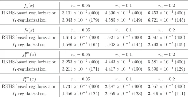
To evaluate the performance of the RKHS-based regularization (5.1) and the `1

-regularization (5.2) in the examples above, we generate 400 points xi ∈R2, 1≤ i≤400,

evenly spaced along its domain axes. For f = f1, f2, f1pw and f2pw, we compute three

groups of noise-polluted function values,yi =f

¡

xi

¢