© APMTAC, Portugal, 2015
MULTILEVEL MONTE-CARLO METHODS APPLIED TO THE
STOCHASTIC ANALYSIS OF AERODYNAMIC PROBLEMS
Gabriel Bugeda 1, Jordi Pons-Prats2
1: Centre Internacional en Metodes Numerics en Enginyeria (CIMNE), & Universitat Politècnica de Catalunya. Barcelona Tech (UPC),
Edificio C1, Gran Capitan, 08034, Gran Capitan, 08034, Barcelona, Spain. Tel. (+34) 934016494 / Fax. (+34) 934016894.
e-mail: [email protected]
2: Centre Internacional en Metodes Numerics en Enginyeria (CIMNE), Edificio C1, Gran Capitan, 08034,
Barcelona, Spain. Tel. (+34) 932057016 / Fax. (+34) 934016517. e-mail: [email protected]
Key Words: Multilevel Monte Carlo Methods, analysis with uncertainties, CFD, finite
elements, RAE2822.
Abstract: This paper demonstrates the capabilities of the Multi-Level Monte Carlo Methods (MLMC) for the stochastic analysis of CFD aeronautical problems with uncertainties. These capabilities are compared with the classical Monte Carlo Methods in terms of accuracy and computational cost through a set of benchmark test cases. The real possibilities of solving CFD aeronautical analysis with uncertainties by using MLMC methods with a reasonable computational cost are demonstrated.
1. INTRODUCTION
Extensive work has been carried out in the development of classical Monte Carlo (MC) methods for stochastic analysis of CFD problems with uncertainties in the data parameters compatible with modern computational techniques (finite element methods, finite volume methods, finite difference and meshless methods). The basic MC method is represented by a procedure with three steps:
1. Generation of samples of the random input parameters with uncertainties in accordance with their probabilistic density function (PDF).
2. For each sample, a deterministic computation is launched and a deterministic output is recorded.
3. The statistical descriptors of the relevant output quantities are computed by combining the results of all deterministic analysis.
The potential of MC method lies in its basic property of convergence to the exact stochastic solution as the number of input samples tends to infinity, making it a reference method to which other approximate techniques can be compared. It is known that MC methods are independent of the physics of the deterministic system under consideration and can handle a large number of uncertainties characterized by important scatters. Monte Carlo methods have the advantage of being non-intrusive and directly applicable to any code, considered as a “black box”. However, two types of requirements have to be accomplished when using MC
2 method in a correct way:
1. The number of deterministic samples to be computed has to be large enough in order to obtain a correct statistical representation of the solution. This number increases in a significant way with the number of uncertainties.
2. The computational grid used for each deterministic numerical analysis has to be fine enough in order to provide numerical results with a controlled level of discretization error. The main consequence of these two requirements is a too high computational cost of classical MC methods for the stochastic analysis of industrial problems with complex geometries and a high number of uncertainties. In order to reduce this computational cost, efficient design of experiment (DoE) sampling techniques, e.g. Latin Hypercube, Halton or Hammersley samplings, have been used. A second option for reducing the computational cost, used in optimization procedures, is to combine MC methods with a surrogate or approximate model, which allows a cheaper evaluation of the deterministic output in step 2. Initially a database is filled with computed solutions based on the complex numerical model. Next the surrogate model is constructed by fitting a response surface in conformity with the available database. The most widely applied techniques for constructing response surfaces are: artificial neuronal networks, Demeulenaere et al. (2004) [2], radial basis functions, Loeven et al. (2007a) [3], Martin and Roge (2009) [4] or Kriging methods, Peter et al. (2007) [5].
A promising new approach, based on a Multi-Level Monte Carlo method (MLMC) has been introduced recently by Giles (2008) [5], Giles and Reisinger (2012) [6], Mishra et al (2011) [6], (2012) [7], which shows great potential for CFD related stochastic analysis. The authors have demonstrated that the MLMC statistical sampling method is a powerful tool in the context of uncertainty quantification for hyperbolic systems of conservation laws. The method appears to be flexible and can be used for different types of uncertain inputs such as random initial data, source terms or flux functions. Moreover, the MLMC method can deal with a very large number of sources of uncertainty. For instance, a computation for shallow water equations with uncertain bottom topography is reported, involving approximately 1000 sources of uncertainty, while being several orders of magnitude more efficient than the standard Monte Carlo (MC) method, without applying surrogate models.
The MLMC method is based on the use of different levels of accuracy for the deterministic analysis and a different number of sampling points for each one. The statistical representation of the result of the MLMC method is ensured by a high number of sampling points analysed with a low level of accuracy whereas the discretization error is controlled by a short number of sampling points analysed with a high level of accuracy. This combination provide very good quality results for the stochastic analysis with a much more reasonable computational cost compared with classical MC method. Details of MLMC method will be provided in section 3 of this paper.
The main objective of this paper is to demonstrate the big performance of using MLMC for the stochastic solution of CFD problems with uncertainties in comparison with classical MC method. This demonstration will come from a comparison of using both methods in the solution of different test cases. Next section shows the influence of the number of deterministic sampling points and the quality of the solution of each deterministic analysis in the quality of the final solution and the corresponding computational cost of a stochastic analysis. Section 3 will provide details about the MLMC method together with a comparison of its performance with the MC method.
3
2. BENCHMARK TEST CASE BY USING CLASSICAL MC METHOD
This section reports the results of a study performed with the MC method for the stochastic analysis of a simple test case. In this study the influence of the number of sampling points and the degree of accuracy used for the deterministic analysis of each one is studied. The degree of accuracy is modified by using different levels of discretization error.
This test case is based on a 2D RAE2822 airfoil geometry and the uncertainties are applied to Angle of Attack (AoA), Mach number (M), and thickness to chord ratio (T/C). Table 1 shows the parameters of the normal PDF of the parameters with uncertainties. The quantities of interest are the coefficients of lift, drag and momentum, or a selection of one of them.
Parameter Mean Deviation
AoA 2,79 0,1
M 0,734 0,005
T/C 1 0,005
Table 1: Definition of uncertainties for the test case. MC method formulates the mean value of a functional as:
EM[Uτn] =M � U1 τk,n M k=1
(1)
Being:
E the mean value expectation M the number of samples U the functional investigated τ the discretization of the functional
n the last timestep of the numerical simulation (just to ensure the numerical convergence of the simulation)
The other 3 statistical moments; namely the variance, skewness and kurtosis can be easily obtain in a similar way from the set of samples.
The whole Monte Carlo procedure can be summarized as: Define the desired number of samples
Calculate the stochastic points derived from the PDF of the input parameters Calculate the value of the functional for each stochastic point
Calculate the statistical moments of the results.
The solver used for the deterministic analysis of each sampling point is an in-house implementation of the Euler equations for CFD, it is called PUMI [11]. The code uses a Galerkin scheme added to a stabilization technique. It is a low computational cost solver for calculating the lift force up to transonic regimes. It was developed under the framework of a European project called REMFI, and it is based in GiD technology for pre and post-processing [12].
4
2.1. Results obtained with classical MC analysis with different levels of discretization
Different MC analysis have been performed using 4 different meshes. Each mesh is used to calculate the behaviour of the statistical moments of the quantity of interest. The objective is to compare the results and the computational cost obtained with each mesh in terms of the number of sampling points and the degree of discretization. In section 3 this will be compared with the use of MLMC method which combines all these levels of discretization. The same set of 500 sampling points for the input parameters with uncertainties has been generated for all 4 meshes using the PDF characteristics shown in Table 1.
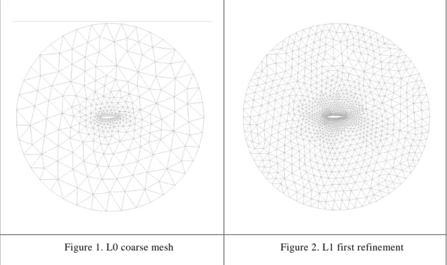
The used meshes can be shown in Figure 1 to Figure 4 and have the following characteristics: L0; Coarse mesh; 318 nodes, 571 triangular linear elements
L1; refinement 1; 1207 nodes, 2284 triangular linear elements L2; refinement 2; 4698 nodes, 9136 triangular linear elements L3; refinement 3; 18532 nodes, 36544 triangular linear elements
Each mesh has been obtained as a refinement of the previous one by subdividing each mesh size h by 2.
5
Figure 3. L2 second refinement Figure 4. L3 third refinement
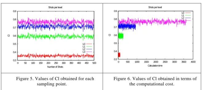
With each of the 4 meshes a full MC analysis has been performed using the generated 500 sampling points. Figure 5 and Figure 6 show the results obtained for Cl from each of the deterministic analyses. Figure 2a show, for each of the 4 meshes, the numerical result for the 500 numerical analyses. It can be seen how, or each mesh, the results of the analyses oscillates around a medium value being this value different for each level of discretization. Obviously, this mean value is depending on the amount of discretization error associated with each mesh being the L3 mesh the one with a larger level of accuracy. Figure 6 shows the same results but now in terms of the computational cost. As it can be seen in Figure 6, the cost of the analyses for the 500 sampling points for the L0 mesh is around 100min (less than 2h), whereas for the L3 mesh it increases to 3800min (more than 60h).
Figure 5. Values of Cl obtained for each
sampling point.
Figure 6. Values of Cl obtained in terms of the computational cost.
0.3 0.4 0.5 0.6 0.7 0.8 0.9 0 50 100 150 200 250 300 350 400 450 500 Cl Number of Shots Shots per level
L0 L1 L2 L3 0.3 0.4 0.5 0.6 0.7 0.8 0.9 0 500 1000 1500 2000 2500 3000 3500 4000 Cl Calculation time Shots per level
L0 L1 L2 L3
6
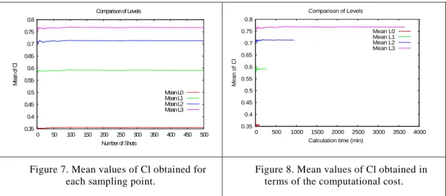
Figure 7and Figure 8 show the evolution of the mean value of Cl. Figure 7shows, for each sampling point (Shot), the mean value of Cl obtained using this and all the previous points. It can be seen how this value converges to a final one after an initial number of sampling points. This final value is different for each level of discretization being the one obtained with the L3 mesh the largest one, as expected. The obtained value with the L0 discretization level is 0,35 whereas for the L3 level is 0,76.
Again, Figure 8shows the same type of information but now in terms of the computational cost.
Figure 7. Mean values of Cl obtained for each sampling point.
Figure 8. Mean values of Cl obtained in terms of the computational cost.
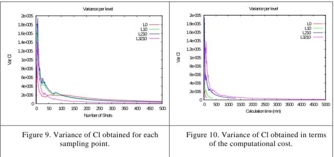
Figure 9 and Figure 10 show the evolution of the variance of Cl with the number of sampling points and for each level of discretization. In Figure 9, for each sampling point the variance computed from this and all previous points is represented. Figure 10 shows a similar information now in terms of the computational cost.
It is normally considered that a MC method has produced a statistically representative result when the variance of the Quantity of Interest (QoI, Cl in this test case) has converged to a minimum value. Figure 4a shows how this convergence takes several hundreds of sampling points for any of the discretization levels, being this the major reason for the high computational cost of MC methods.
0.35 0.4 0.45 0.5 0.55 0.6 0.65 0.7 0.75 0.8 0 50 100 150 200 250 300 350 400 450 500 Mean of C l Number of Shots Comparison of Levels Mean L0 Mean L1 Mean L2 Mean L3 0.35 0.4 0.45 0.5 0.55 0.6 0.65 0.7 0.75 0.8 0 500 1000 1500 2000 2500 3000 3500 4000 M e an of C l
Calculation time (min) Comparison of Levels
Mean L0 Mean L1 Mean L2 Mean L3
7 Figure 9. Variance of Cl obtained for each
sampling point.
Figure 10. Variance of Cl obtained in terms of the computational cost.
2.2. Results obtained with classical MC analysis with discretization based on the number of time-steps
A second set of analysis have been defined. In this case, the discretization was no longer using the mesh size as principal parameter, but the number of time steps of the simulation. The objective is to confirm that any kind of definition of the approximation levels is valid. The time-steps discretization has been considered due to the fact that not required re-meshing, which means a lower computational cost. The first level will use only 500 time-steps, which will lead to a poor approximation of the functional (Cl, as defined previously). The time-step discretization is also following a geometrical progression and the successive levels define this parameter as 500 ∗ 2L, which means that the second level uses 1000 time-steps, the third 2000, and the forth 4000.
Figure 11. Values of Cl obtained for each
sampling point (timestep case).
Figure 12. Values of Cl obtained in terms of the computational cost (timestep case). Figure 11 and Figure 12 show the Cl values along the 500 stochastic samples that have been evaluated. As presented in the mesh discretization case, the lower levels provide a course value of Cl. Regarding the computational cost, the calculation time for each level quickly increases with the accuracy of the level. It is clearly the expected behaviour; the lower the
0 2e-006 4e-006 6e-006 8e-006 1e-005 1.2e-005 1.4e-005 1.6e-005 1.8e-005 2e-005 0 50 100 150 200 250 300 350 400 450 500 Va r C l Number of Shots Variance per level
L0 L10 L210 L3210 0 2e-006 4e-006 6e-006 8e-006 1e-005 1.2e-005 1.4e-005 1.6e-005 1.8e-005 2e-005 0 500 1000 1500 2000 2500 3000 3500 4000 4500 5000 Va r C l
Calculation time (min) Variance per level
L0 L10 L210 L3210 0.3 0.35 0.4 0.45 0.5 0.55 0.6 0.65 0.7 0.75 0.8 0.85 0 50 100 150 200 250 300 350 400 450 500 Cl Number of Shots Shots per level
L0 L1 L2 L3 0.3 0.35 0.4 0.45 0.5 0.55 0.6 0.65 0.7 0.75 0.8 0.85 0 200 400 600 800 1000 1200 1400 1600 Cl Calculation time Shots per level
L0 L1 L2 L3
8 accuracy is, the fastest it computes.
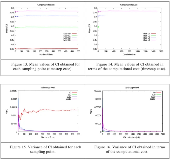
The points in Figure 11 and Figure 12 oscillate around the mean values of each level. These mean values have been plotted in Figure 13 and Figure 14, against number of samples and time. In all four cases, calculating 500 samples, the convergence to the population mean is accurate enough. This is a key point to evaluate the need for more samples.
But the mean value is not the only statistical moment to take into consideration. The variance is also important, and it usually presents more difficulty on quickly converge. Figure 15 and Figure 16 show the evolution of the variance of the samples, against number of samples and time as done in the previous plots. In these figures the variance of the difference between two consecutive levels of discretization is plotted.
It is relevant that the low accuracy discretization, the first level, shows a larger variance than the following levels. It is due to the fact that the first level corresponds to a single level of accuracy, while the following levels are the difference of two levels of accuracy.
Figure 13. Mean values of Cl obtained for each sampling point (timestep case).
Figure 14. Mean values of Cl obtained in terms of the computational cost (timestep case).
Figure 15. Variance of Cl obtained for each sampling point.
Figure 16. Variance of Cl obtained in terms of the computational cost.
3. MULTILEVEL MONTE-CARLO METHOD
As mentioned, the MLMC method is based on a combination of a large number of
0.35 0.4 0.45 0.5 0.55 0.6 0.65 0.7 0.75 0.8 0 50 100 150 200 250 300 350 400 450 500 Mean of C l Number of Shots Comparison of Levels Mean L0 Mean L1 Mean L2 Mean L3 0.35 0.4 0.45 0.5 0.55 0.6 0.65 0.7 0.75 0.8 0 200 400 600 800 1000 1200 1400 1600 Mean of C l Calculation time Comparison of Levels Mean L0 Mean L1 Mean L2 Mean L3 0 5e-005 0.0001 0.00015 0.0002 0.00025 0 50 100 150 200 250 300 350 400 450 500 Va r C l Number of Shots Variance per level
L0 L10 L210 L3210 0 5e-005 0.0001 0.00015 0.0002 0.00025 0 200 400 600 800 1000 1200 1400 1600 1800 2000 Va r C l
Calculation time (min) Variance per level
L0 L10 L210 L3210
9
evaluations with a low level of accuracy with a small number of evaluations with a high level of accuracy. Let’s assume a sequence P0, P1, … which approximates a QoI (PL) with increasing accuracy, but also increasing cost. Due to the linear property of the mean value operator we have (see reference [6])
E[PL] = E[P0] + � E[Pl− Pl−1] L
l=1
(2)
and therefore we can use the following unbiased estimator for E[PL],
E[PL] ≈ N0−1� P0(0,n) N0 n=1 + � �Nl−1� �Pl(l,n)− Pl−1(l,n)� Nl n=1 � L l=1 (3) being:
Nl the number of samples for the l level of accuracy
Pl(l,n) the result of the evaluation of the n sample of the l level of accuracy (notice that the sampling points for each level of accuracy are independent)
If we define Cl and Vl to be the computational cost and the variance obtained for the l level of accuracy, then the overall cost and variance of the multilevel estimator are CL= ∑ NLl=0 lCl and VL= ∑ NLl=0 l−1Vl, respectively.
For a fixed computational cost, the variance is minimised by choosing Nl = λ�Vl/Cl for a value of the Lagrangian multiplier λ.
A typical computer implementation of the MLMC method is as follows: Start L=0,
Estimate Variance Vl defining an initial number of samples Nl
Calculate optimal Nl using Nl = 2ϵ−2�Vlhl�∑ �VLl=0 l/hl�, being hl the computational cost associated to the analysis if each sampling point, and λ λa user-defined tolerance.
Evaluate extra samples if optimal Nl is larger than the initial estimation If L≥2, test convergence using:
max{M−1|Y
L−1|, |YL|} <√21 (M − 1)ϵ
or
|YL− M−1YL−1| <√21 (M2− 1)ϵ
If L<2, or not converged, L=L+1
Go to (2) Estimate Variance Vl defining an initial number of samples Nl
To avoid misunderstandings it should be clarified that what the Multi-Level Monte Carlo method defines as “Level” means the difference of two consecutive levels of discretization. See more details in the next section.
Take a look at references [6][7][8][5] for more details.
3.1. Results obtained with MLMC analysis with different meshes
In this subsection we show the results obtained with the MLMC method applied to the test case described in section 2. The different levels of accuracy correspond with the different meshes described in 2.1. The presented application is based on UMRIDA BC-02 test case
10
[1][2]. The BC-02 test case defines the 2D RAE2822 airfoil geometry as the baseline. It applies uncertainty on Angle of Attack (AoA), Mach number (M), and thickness to chord ratio (T/C). The results presented here uses two set of variables; AoA and M, and also AoA, M and T/C as the uncertain parameters. The quantity of interest for this study is the coefficient of lift.
Working with the AoA and the M number as uncertain parameters, the analysis presented in section 2.1 is fully comparable with the results presented here. On the other hand, when T/C ratio is also included in the analysis, the final results are not equivalent. Let’s start with the first case using AoA and M.
3.1.1. Mesh refinement discretization when AoA and M are stochastically defined
Section 2.1 defines an analysis aimed to understand the results which can be obtained with several levels of discretization based on mesh refinements. The selection of the number of levels and the stochastic samples is not automatic, so the purpose of the present section is to show a fully automatic analysis of MLMC with mesh refinement discretization.
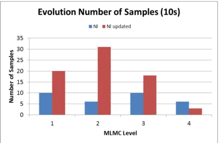
As stated in the description of the method, an initial number of samples msut be evaluated. If 10 initial samples are defined, the method updates the number of samples requiring some additional ones. The evolution of the number of samples, which greatly affects the final computational cost of the method, is described in Figure 17.
Figure 17. Updated number of samples (10 initial samples)
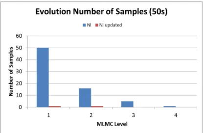
The number of levels and the evolution depicted in Figure 17 are directly dependant on the value λ, which is the Lagragian multiplier in the equation used to update the number of samples. It keeps a strong relationship with the value of the individual computational cost and must be selected accordingly. It ensures the fast and accurate convergence of the method. A wrong selection of the multiplier value can lead to opposite situations; namely a lack of convergence with a complete unaffordable number of samples, or a too fast convergence with a limited number of levels which are not able to get the final mean and variance values. The number of initial samples is also relevant to ensure the accuracy and the low cost of the method. If the previous example is run with 50 initial samples, the evolution of the number of samples is completely different, while the λ and other configuration parameters are kept the same. Figure 18 shows this evolution, where the convergence is straight forward from 50 to
11
the 1, without additional samples to calculate in any of the MLMC levels.
Figure 18. Updating samples for 50 initial ones
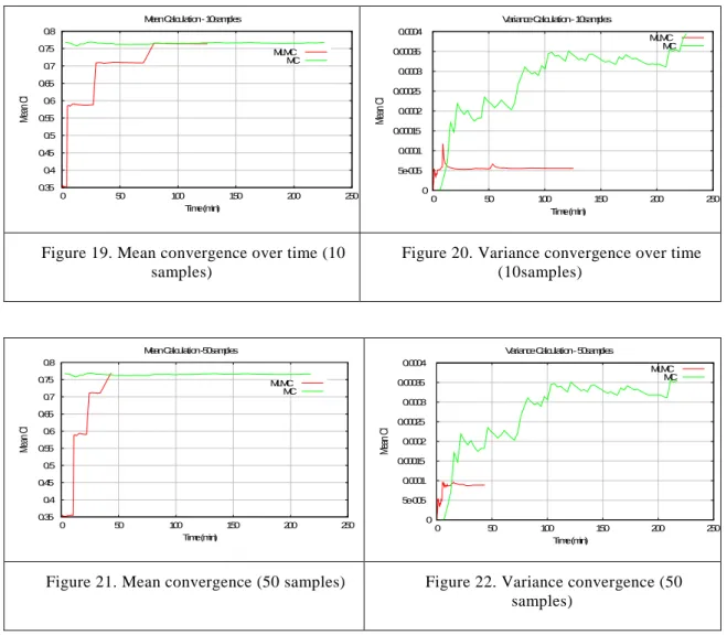
Of course, a relevant analysis to perform is the convergence of the mean and the variance values. The aim of the MLMC is to get those values with a limited computational cost. The following results compare the standard Monte Carlo method with the Multi-level Monte Carlo. Figure 19, Figure 20, Figure 21, and Figure 22 show the convergence history for both cases using 10 and 50 initial samples. All the figures show the history over time, and in comparison with Monte Carlo (MC) method results. It is clear that the convergence is faster with the MLMC than in MC, for both the mean and the variance value. Focusing on the variance, the value is improved leading to a smaller value in the MLMC case. The variance value converges quicker, even in the initial levels already presents a value close to its final converged value. The behaviour of the mean is different, due to the fact each level contributes to reach the final converged value. This contribution is clearly shown in the steps present in the plot. Each step is a new level. The partial time required for each step increases, so the length of each step is also increased, even though the number of samples in each level is reduced.
It is relevant to insist on the fact that the number of initial samples, together with the value of the Lagrangian multiplier λ have a direct effect on the number and evolution of the required samples per level. In addition to these two parameters some tests have demonstrated that the discretization is also an important issue to consider. It does not represent a problem by itself, but if the value of λ leads to a reduced number of levels, then the final value of the QoI could not converge to its real value.
12 Figure 19. Mean convergence over time (10
samples)
Figure 20. Variance convergence over time (10samples)
Figure 21. Mean convergence (50 samples) Figure 22. Variance convergence (50 samples)
3.1.2. Mesh refinement discretization when AoA, M and T/C are stochastically
defined
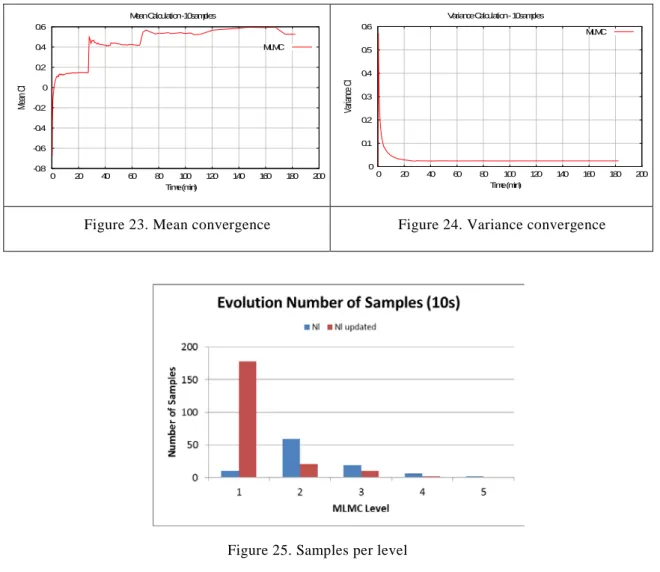
As described in the definition of the BC-02 test case from the UMRIDA project, three uncertain parameters have to be defined; namely the Angle of Attack (AoA), the Mach number (M) and Thickness to Chord ratio (T/C). The behavior of the QoI, the Cl, is similar to what we have seen in the previous analysis. The mean value is converging quite fast, which is important to reduce the computational cost. On the other hand, the variability that the third uncertain parameter introduces can be easily identified on the value of the variance. Figure 23 and Figure 24 are the plot of the convergence history of the mean and variance values. Comparing the value we obtained when defining only two uncertain parameters, the mean has decreased and the variance have increased. The increment of the variance is significantly higher than the decrement of the mean. The increment on the variance was expected due to the additional variability introduced by the new uncertainty, but the decrement of the mean is under investigation to better understand where it comes from.
Figure 25 shows the behavior of the analysis from the point of view of the method. It shows the number of samples defined and updated to fulfil the procedure criteria of convergence. As shown in the previous analysis, the number of samples is reduced in each level.
0.35 0.4 0.45 0.5 0.55 0.6 0.65 0.7 0.75 0.8 0 50 100 150 200 250 Mean Cl Time (min) Mean Calculation - 10samples
MLMC MC 0 5e-005 0.0001 0.00015 0.0002 0.00025 0.0003 0.00035 0.0004 0 50 100 150 200 250 Mean Cl Time (min) Variance Calculation - 10samples
MLMC MC 0.35 0.4 0.45 0.5 0.55 0.6 0.65 0.7 0.75 0.8 0 50 100 150 200 250 Mean Cl Time (min) Mean Calculation -50samples
MLMC MC 0 5e-005 0.0001 0.00015 0.0002 0.00025 0.0003 0.00035 0.0004 0 50 100 150 200 250 Mean Cl Time (min) Variance Calculation - 50samples
MLMC MC
13
Figure 23. Mean convergence Figure 24. Variance convergence
Figure 25. Samples per level
3.2. Results obtained with MLMC analysis with levels of discretization based on the number of timesteps
In this subsection we show the results obtained with the MLMC method applied to the test case described in section 2. Now, the different levels of accuracy correspond with the different levels of discretization described in 2.2, which correspond to the number of timesteps of the finite element analysis.
The selection of the number of time-steps as the discretization criteria is based on the criteria of get a lower computational cost an easy implementation of such a test case.
Several tests have been performed to assess the effect of tolerance of the mean and the variance on the stopping criteria, as well as to assess the effect of defining the λ value which is used to calculate the updated number of samples in each level. Table 1 describes the values defined in each test case. It is clear that the three parameters will influence the convergence ratio, and will determine the final amount of samples in each level as well as the number of levels to be calculated. It is expected that the effect of the two tolerances will mainly determine the number of levels, while the λ value will determine the number of samples.
-0.8 -0.6 -0.4 -0.2 0 0.2 0.4 0.6 0 20 40 60 80 100 120 140 160 180 200 Mean Cl Time (min) Mean Calculation -10samples
MLMC 0 0.1 0.2 0.3 0.4 0.5 0.6 0 20 40 60 80 100 120 140 160 180 200 Var ianc e C l Time (min) Variance Calculation - 10samples
14 Test Initial Samples Tolerance of the Mean Tolerance of the Variance Lambda λ
DMx 10 1e-6 1e-9 1e-2
BKr 50 1e-6 1e-6 1e-2
DBe 10 1e-6 1e-9 1e-3
D1Kr 50 1e-6 1e-9 1e-3
Table 1. Set-up of the MLMC tests
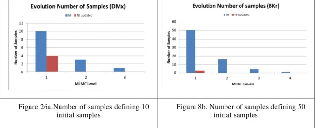
The number of initial samples is not relevant to determine the convergence of the method, from the point of view of reducing the number of samples of the successive levels. Figure 26a and b show the evolution of the DMx and BKr test cases. Both of them were using λ equal to 10-2. For low values of epsilon the updated number of samples (Nl) is usually lower than the calculated number of samples, which means than no additional samples should be calculated. Figure 27a and b show the evolution of required samples when λ equal to 10-3 for 10 and 50 initial samples. In these cases, the larger value of λ leads to the need to calculate more samples than those initially defined, increasing the final total cost of the analysis. If the value of λ is larger (10-4 in some cases) the number of samples presents a complete lack of convergence to a minimum. The additional samples to calculate rapidly increase to an absolutely unaffordable number of samples (millions of samples for instance), which means the analysis should be discarded and stopped.
Figure 26a.Number of samples defining 10 initial samples
Figure 8b. Number of samples defining 50 initial samples
15 Figure 27a.Number of samples defining 10
initial samples
Figure 9b. Number of samples defining 50 initial samples
Let’s focus on the convergence of the mean value and the value of the variance of the quantity of interest (QoI), which in this case is the mean and the variance of the Cl coefficient. One can easily realize that a larger total number of samples is obtained when a larger number of initial samples are defined. It is true that the final convergence is also influenced by the stopping criteria the user defines. On the other hand, the accuracy of the method, compared to a standard Monte Carlo analysis, is greater with a large number of samples. Figure 28a and b, and Figure 29a and b show the evolution of the mean value over the calculation time and the total number of samples. This evolution is compared with the equivalent Monte Carlo analysis (with equal number of samples). The first point to highlight is the reduction in cost we get using the Multi-Level Monte Carlo. Even with the same number of samples the final cost is reduced thanks to the fact that the individual cost of each sample is also reduced. On the other hand, the accuracy in both cases is similar. To get a MLMC final value closer to the MC one greatly depends on the intrinsic random character of the method. One could conclude that the gain using MLMC is ok, but could still prefer using MC.
Figure 28a.Evolution of Mean Value defining 10 initial samples
Figure 10b. Evolution of Mean Value defining 50 initial samples
0.55 0.6 0.65 0.7 0.75 0.8 0 5 10 15 20 25 30 35 40 45 Mean Cl Time (min) Mean Calculation - DMx MLMC MC 0.55 0.6 0.65 0.7 0.75 0.8 0 50 100 150 200 250 Mean Cl Time (min) Mean Calculation - BKr MLMC MC
16 Figure 29a.Evolution of Mean Value with 10
initial samples
Figure 11b. Evolution of Mean value with 50 initial samples
Then, if we analyse the variance, a greater difference between the two methods can be identified. Figure 30 and Figure 31 show the evolution of the variance along the analysis, the first over the time and the second over the number of total samples. The benefit of MLMC is now clear; the convergence of the variance is obtained easily with the MLMC method, for the same number of calculated samples. As the figures show, MLMC variance takes less time to better converge than in the MC analysis.
Figure 30a.Evolution of Variance defining 10 initial samples
Figure 12b. Evolution of Variance defining 50 initial samples
Figure 31a.Evolution of Variance with 10 initial samples
Figure 13b. Evolution of Variance with 50 initial samples 0.55 0.6 0.65 0.7 0.75 0.8 0 2 4 6 8 10 12 14 Mean Cl Shots - Evaluations Mean Calculation - DMx MLMC MC 0.55 0.6 0.65 0.7 0.75 0.8 0 10 20 30 40 50 60 70 80 Mean Cl Shots - Evaluations Mean Calculation - BKr MLMC MC 0 5e-005 0.0001 0.00015 0.0002 0.00025 0 5 10 15 20 25 30 35 40 45 Mean Cl Time (min) Variance Calculation - DMx MLMC MC 0 5e-005 0.0001 0.00015 0.0002 0.00025 0.0003 0.00035 0.0004 0 50 100 150 200 250 Mean Cl Time (min) Variance Calculation - BKr MLMC MC 0 5e-005 0.0001 0.00015 0.0002 0.00025 0 2 4 6 8 10 12 14 Mean Cl Shots - Evaluations Variance Calculation - DMx MLMC MC 0 5e-005 0.0001 0.00015 0.0002 0.00025 0.0003 0.00035 0.0004 0 10 20 30 40 50 60 70 80 Mean Cl Shots - Evaluations Variance Calculation - BKr MLMC MC
17
4. CONCLUSIONS
The presented work is introducing an implementation of the Multi-Level Monte Carlo method. The work presents an academic application based on the UMRIDA BC-02 test case, defining as the discretization parameter the mesh size or the number of time-steps of the simulation. The results show the benefit of the Multi-Level Monte Carlo in regards of the variance converge and the computational cost. The Multi-Level Monte Carlo method is able to reduce the computational cost, reducing the required number of samples to be calculated and the individual cost of each sample. The values of the two principal statistical moments are optimized for specific values of the parameter λ, an internal parameter used for the update of the number of samples. With the correct settings, the method easily converge, requiring a small number of levels, and a small number total samples. Further investigations are going on to determine the relationship between the Lagrangian multiplier λ, and several parameters of the analysis such the individual computational cost of each sample, the initial number of samples, for instance.
ACKNOWLEDGEMENT
This work has been supported by the 7th Framework program FP7, under the UMRIDA project (grant agreement n° 605036).
REFERENCES
[1]. Demeulenaere et al. (2004), Demeulenaere A., Ligout A., Hirsch Ch. (2004), Application of Multipoint Optimization to the Design of Turbomachinery Blades, paper GT-2004-53110, Proceedings of ASME Turbo Expo 2004 Power for Land, Sea and Air, June 14-17, 2004, Vienna, Austria.
[2]. Loeven et al. (2007a), Loeven, A., Witteveen, J., Bijl, H. (2007a), A Probabilistic Radial Basis Function Approach for Uncertainty Quantification, Paper 35, NATO RTO-AVT-147 Symposium on ―Computational Uncertainty in Military Vehicle Design‖, 3-6th December 2007, Athens, Greece
[3]. Martin and Roge (2009), Martin, L., Rogé, G. (2009), "Management of uncertainties in the Framework of Aerodynamic Design", Symposium "Uncertainty Quantification in Computational Science and Engineering", Delft University of Technology, the Netherlands.
[4]. Peter et al. (2007). Peter, J., Marcelet, M., Burguburu, S., Pediroda, V. (2007), Comparison of surrogate models for the actual optimization of a 2D turbomachinery flow, Proceedings of the 7th WSEAS International Conference on SIMULATION, MODELLING AND OPTIMIZATION (SMO '07), ISSN: 1790-5117 ISBN: 978-960-6766-05-3, pg. 46
[5]. Giles M.B., (2008) Multilevel Monte Carlo path simulation, M.B. Giles. Multilevel Monte Carlo path simulation. Oper. Res., 256:981-986.
[6]. M.B. Giles and C. Reisinger. (2012) Stochastic _nite di_erences and multilevel Monte Carlo for a class of SPDEs in _nance. SIFIN, 1(3):575-592.
[7]. Mishra et al (2011), Mishra S., Schwab Ch., Sukys J., (2011), Multi-level Monte Carlo finite volume methods for nonlinear systems of conservation laws in multi-dimensions. J. Comp. Phys., 231(8), pp 3365–3388.
18
Carlo finite volume methods for uncertainty quantification in nonlinear systems of balance laws, Research Report No. 2012-08, April 2012, Seminar f¨ur Angewandte Mathematik ETH Zurich.
[9]. UMRIDA project website; www.umrida.eu/, last visited 20/03/2015 [10]. Wunsch, D., UMRIDA BC-02 test case definition, project technical report
[11]. Flores R., Ortega E., 2007, PUMI: an explicit 3D unstructured finite element solver for the Euler equations. CIMNE 2007