Option pricing with regime switching by trinomial tree method

(1)

Title Option pricing with regime switching by trinomial tree method

Author(s) Yuen, FL; Yang, H

Citation Journal Of Computational And Applied Mathematics, 2010, v. 233_{n. 8, p. 1821-1833}

Issued Date 2010

URL http://hdl.handle.net/10722/124160

(2)

Option Pricing with Regime-switching by

Trinomial Tree Method

Fei Lung Yuen

a

and

Hailiang Yang

b

Department of Statistics and Actuarial Science

The University of Hong Kong

Pokfulam Road, Hong Kong

a

telephone number: 852-2859-2466

b

telephone number: 852-2857-8322

(3)

Abstract

We present a fast and simple tree model to price simple and exotic options in Markov

Regime Switching Model (MRSM) with multi-regime. We modify the trinomial

tree model of Boyle (1986) by controlling the risk neutral probability measure in

different regime states to ensure that the tree model can accommodate the data

of all different regimes at the same time preserve its combining tree structure. In

MRSM, the market might not be complete, therefore we provide some ideas and

discussions on managing the regime switching risk as a support of our results.

Keywords: Trinomial method, regime switching, option pricing, exotic op-tions, hedging risk of regime-switching.

(4)

1 Introduction

In the past decades, option pricing has become one of the major areas in modern financial theory and practice. Since the introduction of the celebrated Black-Scholes option-pricing model, which assumes that the underlying stock price follows a geometric Brownian mo-tion (GBM), there is an explosive growth in trading activities on derivatives in the world-wide financial markets. The main contribution of the seminal work of Black and Scholes (1973) and Merton (1973) is the introduction of a preference-free option-pricing formula which does not involve an investor’s risk preferences and subjective views. Due to its com-pact form and computational simplicity, the Black-Scholes formula enjoys great popularity in the finance industries. One important economic insight underlying the preference-free option-pricing result is the concept of perfect replication of contingent claims by contin-uously adjusting a self-financing portfolio under the no-arbitrage principle. Cox, Ross and Rubinstein (1979) provide further insights into the concept of perfect replication by introducing the notion of risk-neutral valuation and establishing its relationship with the no-arbitrage principle in a transparent way under a discrete-time binomial setting.

The Black-Scholes’ model has been extended in various ways. Among those gener-alizations, the Markov regime-switching model (MRSM) has recently become a popular model. This model was first introduced by Hamilton (1989). The MRSM allows the parameters of the market model depending on a Markov chain, and the model can reflect the information of the market environment which cannot be modeled solely by linear Gaussian process. The Markov chain can ensure that the parameters change according to the market environment and at the same time preserve the simplicity of the model. It is also consistent with the efficient market hypothesis that all the effects of the information about the stock price would reflect on the stock price. However, when the parameters of the stock price model are not constant but governed by a Markov chain, the pricing of the options becomes complex.

There are many papers about option pricing under the regime-switching model. Naik (1993) provides an elegant treatment for the pricing of the European option under a regime-switching model. Buffington and Elliott (2002) tackle the pricing of the European option and the American option using the partial differential equation (PDE) method. Boyle and Draviam (2007) consider the the price of exotic options under regime switching using the PDE method. The PDE has become the focus of most researchers as it seems to be more flexible in pricing. However, if the number of regime states is large, and we need to solve a system of PDEs with the number of PDEs being the number of the states of the Markov chain, and there is no close form solution if the option is exotic, then the numerical method to solve a system of PDEs is complex and computational time could be long. In practice, we prefer a simple and fast method. For the European option, Naik (1993), Guo (2001) and Elliott, Chan and Siu (2005) provide an explicit price formula. Mamon and Rodrigo (2005) obtain the explicit solution to European options in regime-switching economy by considering the solution of a system of PDEs. All the close form solutions depend on the distribution of occupation time which is not easy to obtain.

Since the binomial tree model was introduced by Cox, Ross and Rubinstein (1979), the lattice model has become one of the best methods to calculate the price of simple options like the European option and the American option. This is mainly due to the lattice method being simple and easy to implement. Various lattice models have been suggested after that, see, for example, Jarrow and Rudd (1983) and Boyle (1986). The

(5)

Trinomial tree model of Boyle (1986) is highly flexible, and has some important properties that the binomial model lacks. The extra branch of the trinomial model gives one degree of freedom to the lattice and makes it very useful in the case of the regime switching model. Boyle and Tian (1998) use this property of the trinomial tree to price the double barrier option, and propose an interesting method to eliminate the error in pricing barrier options. Bollen (1998) uses a similar idea to construct an efficiently combined tree. Boyle (1988) uses a tree lattice to calculate the price of derivatives with two states. Kamrad and Ritchken (1991) suggest a 2k+ 1 branches model fork sources of uncertainty. Bollen (1998) constructs a tree model which is excellent for solving the price of the European option and the American option in a two-regime situation. The Adaptive Mesh Model (AMM) invented by Figlewsho and Gao (1999) greatly improves the efficiency of lattice pricing. Aingworth, Das and Motwani (2006) use a lattice with a 2k-branch to study the

k-state regime switching model. However, when the number of states is large, the degree of efficiency of the tree models mentioned above is not high. In this paper we propose a trinomial tree method to price the options in a regime switching model. The trinomial tree we propose is a combining tree, with the idea that instead of changing the volatility if the regime state changes, we change the probability, so the tree is still combining. Since we are using a combining tree, the computation is very fast and very easy to implement. The market is incomplete when we use a regime switching process to model the price dynamics of the underlying stock. The no arbitrage price of the derivative security is not unique if the market is incomplete. There are many different methods help us to determine the price of the options in such case. Elliott, Chan and Siu (2005) use the Esscher transform to obtain the no arbitrage price. Guo (2001) introduces the change-of-state contracts to complete the market. Naik (1993) shows that the price of options can also be found by fixing the market price of risks. In the MRSM of Buffington and Elliott (2002), the stock is a continuous process and pricing jump risk seems to be not appropriate. In the last section of this paper, we provide a discussion on hedging the risk in the regime-switching model.

2 Modified Trinomial Lattice

The model setting in this section is based on the work of Buffington and Elliott (2002). We let T be the time interval [0, T] that is being considered. {W(t)}t∈T is a standard

Brownian motion. {X(t)}t∈T is a continuous time Markov chain with finite state space

X := (x1, x2, . . . , xk), which represents the economic condition.

LetA(t) = [aij(t)]i,j=1,...,k be the generator matrix of the Markov chain process. There

are two investment securities available to the investors in the market in our model, one is the bond and the other one is the stock. The risk free interest rate is denoted by {rt =r(X(t))}t∈T which depends only on the current state of economy. The bond price

process {B(t)}t∈T will satisfy the equation:

dB(t) = rtB(t)dt, B(0) = 1 (2.1)

The rate of return and the volatility of the stock price process are denoted by {µt =

µ(X(t))}t∈T and{σt =σ(X(t))}t∈T respectively. Similar to the interest rate process, they

(6)

modulated geometric Brownian motion. Then, we have

dS(t) =µtS(t)dt+σtS(t)dW(t). (2.2)

Let Z(t) = ln(S(t)/S(0)) be the cumulative return of the stock, in time interval [0, T]. Then, under the risk neutral probability, the dynamic of the stock price is

dS(t) = rtS(t)dt+σtS(t)dW(t), (2.3) S(t) = S(u) exp{Z(t)−Z(u)}, (2.4) Z(t) = Z t 0 rt− 1 2σ 2 t ds+ Z t 0 σsdW(s). (2.5)

In this paper, we propose a trinomial tree method to price options in the market mentioned above. We first present the construction of the proposed tree model.

In the CRR binomial tree model, the ratios of changes of the stock price are assumed to beeσ

√

∆t _and _e−σ√∆t_{, respectively. The probabilities of getting up and down are specified}

so that the expected increasing rate of the stock price matches the risk free interest rate. In the trinomial tree model, with constant risk free interest rate and volatility, the stock price is allowed to remain unchanged, or go up or go down by a ratio. The upward ratio must be greater than eσ√∆t _{so as to ensure that the risk neutral probability measure}

exists. Let πu, πm, πd be the risk neutral probabilities corresponding to when the stock

price increases, remains the same and decreases, respectively, ∆t be the size of time step in the model, r be the risk free interest rate, then,

πueλσ √ ∆t₊_π m+πde−λσ √ ∆t ₌ _er∆t _and _(2.6) (πu+πd)λ2σ2∆t = σ2∆t, (2.7)

where λ should be greater than 1 so that the risk neutral probability measure exists. In the literature, the common values ofλ are √3 (Figlewski and Gao (1999) and Baule and Wilkens (2004)) and √1.5 (Boyle (1988) and Kamrad and Ritchken (1991)). After fixing the value of λ, the risk neutral probabilities can be calculated and the whole lattice can be constructed.

However, in the multi-state MRSM, the risk free interest rate and the volatility are not constant. They change according to the Markov chain. In this case, a natural way is to introduce more branches into the lattice so that extra information can be incorporated in the model. For example, Boyle and Tian (1988), Kamrad and Ritchken (1991) construct tree to price options of multi-variable. Aingworth, Das and Motwani (2006) use 2k-branch to study k-state model. However, the increasing number of branches makes the lattice model more complex, Bollen (1998) suggests an excellent combining tree with a tree based model to solve the option prices of the two-regime case, but for multi-regime states, the problem still cannot be solved effectively.

In this paper we propose a different way to construct the tree. Instead of increasing the number of branches, we change the risk neutral probability measure if the regime state changes. In this manner, we can keep the trinomial tree a combining one. The method relies greatly on the flexibility of the trinomial tree model, and the core idea of the multi-state trinomial tree model here is to change probability rather than increasing the branches of the tree.

(7)

Assuming that there are k states in the Markov regime switching model, the cor-responding risk free interest rate and volatility of the price of the underlying asset be

r1, r2, . . . , rk and σ1, σ2, . . . , σk respectively. The up-jump ratio of the lattice is taken to

be eσ√∆t_{, for a lattice which can be used by all regimes, where}

σ > max

1≤i≤kσi. (2.8)

For the regime i, letπ_ui, π_mi , π_di be the risk neutral probabilities corresponding to when the stock price increases, remains the same and decreases, respectively. Then, similar to the simple trinomial tree model, the following set of equations can be obtained for each 1≤i≤k: πi_ueσ √ ∆t₊_πi m+π i de −σ√∆t ₌ _eri∆t _and _(2.9) (π_ui +π_di)σ2∆t = σ_i2∆t. (2.10)

If λi is defined as σ/σi for each i, then, λi > 1 and the values of πui, πmi , πid can be

calculated in terms of λi: π_mi = 1−σ 2 i σ2 = 1− 1 λ2 i (2.11) π_ui = e ri∆t₋_e−σ √ ∆t₋₍₁₋₁_/λ2 i)(1−e−σ √ ∆t₎ eσ√∆t₋_e−σ√∆t (2.12) π_di = e σ√∆t₋_eri∆t−₍₁−₁_/λ2 i)(eσ √ ∆t₋₁₎ eσ√∆t₋_e−σ√∆t . (2.13)

Therefore, the set of risk neutral probabilities depends on the value of σ. In order to ensure that σ is greater than all σi, one possible value we suggest is

σ = max

1≤i≤kσi+ (

√

1.5−1)¯σ (2.14)

where ¯σ is the arithmetic mean of σi. Another possible suggestion is that ¯σ be the root

mean square. These suggestions are based on the values used in the binomial tree and trinomial tree models in the literature. The idea is try to find a value of σ, such that the convergence speed of the prices using the tree to the value of the price obtained using the continuous model is fast. We believe that the convergence difference between using the arithmetic mean and using the root mean square for the ¯σ is not significant. If the values of σi greatly deviate from one another, the selection of σ will be more important, and

some amendments could be made on this model. We will discuss this problem in Section 4. In this section, σi are assumed to be not greatly different from each other.

After the whole lattice is constructed, the main idea of the pricing method is presented here. We assume T to be the expiration time of the option, N to be the number of time steps, then ∆t =T /N. At time step t, there are 2t+ 1 nodes in the lattice, the node is counted from the lowest stock price level, andSt,n denotes the stock price of thenth node

at time step t. As all the regimes share the same lattice and the regime state cannot be reflected by the position of the nodes, each of the nodes has k possible derivative’s price corresponding to the regime state at that node. Let Vt,n,j be the value of the derivative

(8)

The transition probability of the Markov chain can be obtained from the generator matrix. The generator matrix is assumed to be a constant matrix in this section. pij(∆t)

is defined as the transition probability from regime state ito regime state j for the time interval with length ∆t. For simplicity, it is denoted by pij. If the generator matrix is

assumed to be a constant matrix and denoted by A, the transition probability matrix, denoted by P, can be found by the following equation:

P(∆t) =    p11 · · · p1k .. . . .. ... pk1 · · · pkk   =e A∆t₌_I₊ ∞ X l=1 (∆t)lAl/l!. (2.15)

With the transition probability matrix, the price of the derivative at each node can be found by iteration. We start from the expiration time, for example, for a European call option with strike price K,

VN,n,i = (SN,n−K)+ for all states i (2.16)

where SN,n=S0exp[(n−1−N)σ

√ ∆t].

We assume that the Markov chain is independent of the Brownian motion, thus the transition probabilities will not be affected by changing the probability measure from the physical probability to the risk neutral measure.

With the derivative price at expiration, using the following equation recursively:

Vt,n,i = e−ri∆t " _k X j=1 pij(πuiVt+1,n+2,j+πmi Vt+1,n+1,j+πidVt+1,n,j) # , (2.17)

the price of the option under all regimes can be obtained.

The regime switching imposes an additional risk in the securities market. When pricing the derivatives, we need to consider these additional risks. Due to regime switching, the market becomes incomplete, so the no-arbitrage price of the derivatives is not unique in this market. In the literature, there are usually two ways to treat additional risks from regime switching, either do not pricing the regime switching risk, or introduce change-of-state contracts into the model (see Guo (2001) for the second way). If we do not price the regime switching risk, the model is simple and easy to deal with. However, some derivatives will benefit if we do not price the risk while other derivatives may suffer. The price of the derivatives depends on the initial regime of the underlying security, the transition probabilities and the structure of the derivatives. Since it is hard to choose appropriate transition probabilities, it is not unreasonable, in practice, to choose not pricing the regime switching risk as long as there is no arbitrage opportunity in the market. In our model, only the underlying asset and the bond are used for hedging the risk, and the market is not complete. Although new securities, such as change-of-state contracts can be introduced into the model to complete the market, the regime refers to the macroeconomic condition, this kind of systematic risk is the insurance companies not willing to take. Therefore, in this paper, we assume that there are no suitable change-of-state contracts in the market. The risk premium comes from the risk of the Brownian motion only when we are changing probability to the risk neutral probability measure.

When we price the American option, the value of the option at each node under different regimes can be compared with the payoff of exercising the option immediately, and the

(9)

larger value will be used as the price for iteration. The calculation is similar to the valuation of the American option in the simple lattice model.

The idea of Boyle and Tian (1998) can be applied for the barrier option here. The whole lattice is constructed from the lower barrier. As the initial price of the underlying asset is not necessarily at the grid, a quadratic approximation will be used to calculate the price of the down-and-out option. The price of a down-and-in option can be found using the idea that the sum of the down-and-out option and the down-and-in option is a vanilla option. For a double barrier option, we use the flexibility of the trinomial tree lattice to make both the upper and lower barrier be on the node level by making a fine adjustment of σ’s value. The price of the curved barrier option and the discrete-time barrier option can also be obtained using a similar method by Boyle and Tian (1998).

We assume that the regime is observable, and the payoff of the derivatives might depend on the regime state. In our model, the prices of the derivative under all regimes can be found in each node, so the model is also applicable to the case that the derivative payoffs depending on the regime state.

3 Numerical Results and Analysis

Based on the model introduced in the last section, simple computer programmes can be used to calculate the prices of various options in different regimes. In this section we study the European option, the American option, the down-and-out barrier option, the double barrier option, and prices of these options are calculated using the multi-state trinomial tree. Our study gives us some insights about the price of derivatives in MRSM and the effects of regime switching. First of all, the model is tested by comparing with the results given by Boyle and Draviam (2007).

Table 1 shows that the option price obtained by using the trinomial lattice is very close to the value obtained by using the analytical solutions derived in Naik (1993), and also close to those obtained using partial differential equation in Boyle and Draviam (2007). This verifies that the trinomial tree model proposed in this paper is applicable.

We now study the values of different types of options in a regime-switching model. The underlying asset is assumed to be a stock with the initial price of 100, following a geometric Brownian motion of two-regime model with no dividend. In regime 1, the risk free interest rate is 4% and the volatility of stock is 0.25; in regime 2, the risk free interest rate is 6% and the volatility of stock is 0.35. All options expire in one year with a strike price equal to 100. The generator for the regime switching process is taken to be

−0.5 0.5 0.5 −0.5

.

The transition probabilities of the branch of state up, middle and down with 20 time steps are 0.177003, 0.641304 and 0.181693 in regime 1; and 0.351844, 0.296956 and 0.3512 in regime 2, respectively. These values depend on the size of time step, but the values with other sizes of time step are not much different from these values because the time step is small in general. The values in 20-step case can already give the idea of the size of transition probabilities. We study the numerical results to see if there are any special

(10)

Table 1: Comparison of different methods in pricing the European call option in MRSM

European Call OptionI

Regime 1 Regime 2

S0 Naik B&D Lattice Naik B&D Lattice 94 5.8620 5.8579 5.8615 8.2292 8.2193 8.2297 96 6.9235 6.9178 6.9229 9.3175 9.3056 9.3181 98 8.0844 8.0775 8.0827 10.4775 10.4647 10.4772 100 9.3401 9.3324 9.3369 11.7063 11.6929 11.7049 102 10.6850 10.6769 10.6828 13.0008 12.9870 13.0001 104 12.1127 12.1045 12.1108 14.3575 14.3436 14.3571 106 13.6161 13.6082 13.6143 15.7729 15.7591 15.7725 European Call OptionII

Regime 1 Regime 2

S0 Naik B&D Lattice Naik B&D Lattice

94 6.2748 6.2705 6.2760 7.8905 7.8844 7.8943 96 7.3408 7.3352 7.3422 8.9747 8.9680 8.9789 98 8.5001 8.4938 8.5010 10.1335 10.1264 10.1374 100 9.7489 9.7423 9.7489 11.3641 11.3568 11.3673 102 11.0820 11.0755 11.0833 12.6631 12.6659 12.6674 104 12.4937 12.4877 12.4959 14.0267 14.0197 14.0317 106 13.9777 13.9726 13.9805 15.4510 15.4446 15.4565

†S0 is the initial stock price and the strike price is set to be 100. The volatilities of the stock in regime 1 and regime 2 are 0.15 and 0.25, respectively. The option has maturity 1 year and the lattice is set to

have 1000 time steps. The generators of the regime switching process are

  −0.5 0.5 0.5 −0.5   and   −1 1 1 −1 

(11)

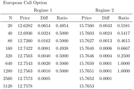
Table 2: Pricing the European call option with the trinomial tree

European Call Option

Regime 1 Regime 2

N Price Diff Ratio Price Diff Ratio 20 12.6282 0.0654 0.4954 15.7560 0.0043 0.5581 40 12.6936 0.0324 0.5000 15.7603 0.0024 0.5417 80 12.7260 0.0162 0.5000 15.7627 0.0013 0.4615 160 12.7422 0.0081 0.4938 15.7640 0.0006 0.6667 320 12.7503 0.0040 0.5000 15.7646 0.0004 0.2500 640 12.7543 0.0020 0.5000 15.7650 0.0001 1.0000 1280 12.7563 0.0010 0.5000 15.7651 0.0001 1.0000 2560 12.7573 0.0005 15.7652 0.0001 5120 12.7578 15.7653

†N is the number of time steps used in calculation. Diff refers to the difference in price calculated using various numbers of time steps and ratio is the ratio of the difference.

characteristics of the prices of these derivatives and the convergence properties of the model.

Tables 2 and 3 show that the convergence rate of the European call and the European put options are fast. We know that the price of the derivative using the CRR model converges to the corresponding price under the simple geometric Brownian motion model, and that the speed of convergence can have an order 1, that is the error of the price is halved if the number of time steps is doubled (Baule and Wilkens (2004) and Omberg (1987)). We can see from the tables that most of the ratios shown in the tables are closed to 0.5. However, it is not the case for the European call option when the number of iterations is large for regime 2. This is because the approximation errors for the two regimes are different. Boyle (1988) shows that using the trinomial tree model, the approximation error is smaller if the three risk neutral probabilities of the trinomial model are almost equal with same number of time steps. In our case, we can see that the risk neutral probabilities of regime 1 are not as close as those of regime 2. Therefore, in regime 2, the change in prices is smaller which implies a smaller approximation error as can be seen from the numerical results in the tables. The differences between the price changes for regime 2 are less than one-tenth of that for regime 1 most of the time. However, the prices of the asset in both regimes affect one another. The larger pricing error in regime 1 affects the accuracy of the price in regime 2. The result is that the value in regime 2 converges in a faster, but more unstable way. On the other hand, the error in regime 2 is smaller compared with that in regime 1; thus the convergence patterns in regime 1 are more stable. Moreover, the change of prices in regime 2 is smaller when the number of time steps is large. The round off error then becomes significant.

When we apply put-call parity to each of the regimes, the interest rate implied in two regimes are 4.37% and 5.63%, respectively, in the 5120 time steps case. This is reasonable, first, because both of them are between 4% and 6%, and the interest rate implied by the

(12)

Table 3: Pricing the European put option with the trinomial tree

European Put Option

Regime 1 Regime 2

numerical results in regime 1 is closer to the rate in regime 1 while the same happens for regime 2. Interestingly, the deviations between the current interest rate and the interest rate implied by the put-call parity in both regimes are equal to 0.37%. This is because of the symmetry of the two regimes in terms of the transition probabilities.

The result of the American option is similar to that of the CRR model. The prices of the American call option found by the modified trinomial model is the same as the European call option. It is consistent with the understanding that the American call option is always not optimal to be exercised before expiration if there is no dividend being distributed. We know that this result is also true for MRSM. The prices of the American put option in the table are larger than those of the European option, meaning that early exercise of the option is preferred sometime and there may be some situations when we have to exercise the American put option before expiration.

The convergence pattern of the American put option is more complicated than the European one. The rate of convergence for the regime 2 is very fast, even faster than that of the European put option. It is hard to give a concrete reason for this, but the fast convergence might be because when it is American option, the put option may be exercised somewhere before the maturity time, so the approximation error is smaller compared to that for the European option case. The convergence pattern of regime 2 is highly unstable, which is consistent with the results for the European option case; the much larger error in regime 1 affects the convergence of the price in regime 2.

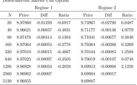
For the down-and-out barrier call option, the prices found in both regimes are smaller than those of the European call option due to the presence of the down-and-out barrier. The prices in the two regimes are closer to each other compared with those of the European option. Although the volatility of regime 2 is greater and has a higher chance to achieve a higher value at expiration, the high volatility also increases the chance of hitting the down-and-out barrier, and thus eliminates its advantage. The convergence pattern of the barrier option is very complicated. It might be the effect of quadratic approximation errors in pricing barrier options. It is difficult to get any conclusions from the numerical

(13)

Table 4: Pricing the American call option with trinomial tree

American Call Option

Regime 1 Regime 2

Table 5: Pricing the American put option with the trinomial tree

American Put Option

Regime 1 Regime 2

N Price Diff Ratio Price Diff Ratio 20 8.80315 0.05236 0.5107 10.8942 0.0007 2.5714 40 8.85551 0.02674 0.4862 10.8949 0.0018 0.1111 80 8.88225 0.01300 0.4869 10.8967 0.0002 0.5000 160 8.89525 0.00633 0.4945 10.8969 0.0001 0.0000 320 8.90158 0.00313 0.4984 10.8970 0.0000 N/A 640 8.90471 0.00156 0.4936 10.8970 0.0000 N/A 1280 8.90627 0.00077 0.4935 10.8970 0.0000 N/A 2560 8.90704 0.00038 10.8970 0.0000 5120 8.90742 10.8970

(14)

Table 6: Pricing the down-and-out barrier call option with the trinomial tree

Down-and-out Barrier Call Option

Regime 1 Regime 2

N Price Diff Ratio Price Diff Ratio

20 8.97860 -0.01239 -0.6917 9.73967 -0.02790 0.0487 40 8.96621 0.00857 -0.4831 9.71177 -0.00136 4.9779 80 8.97478 -0.00414 0.1304 9.71041 -0.00677 0.3840 160 8.97064 -0.00054 -0.2778 9.70364 -0.00260 0.3269 320 8.97010 0.00015 -6.4667 9.70104 -0.00085 1.2588 640 8.97025 -0.00097 -0.3505 9.70019 -0.00107 0.0748 1280 8.96928 0.00034 -0.2059 9.69912 -0.00008 2.1250 2560 8.96962 -0.00007 9.69904 -0.00017 5120 8.96955 9.69887

The barrier level is set as 90.

results. However, we can see that apart from converging uniformly in one direction, the values of the option found in regime 1 are oscillating and the differences still have a decreasing trend in absolute value.

The price of the double barrier option can also be obtained by the trinomial model. The method suggested by Boyle and Tian (1998) is adopted here. The lattice is built from the lower barrier and touches the upper barrier by controlling the value ofσ used in the lattice. Table 7 shows the price of the double barrier option with different numbers of time steps used. The lower barrier is set as 70 and the upper barrier is set as 150. The values decrease progressively and converge. Table 8 summarizes the value of the double barrier options with different barrier levels using 1000 time steps. When the difference between the upper and lower barriers is smaller, the price of the options will be lower as there is a bigger chance of touching the barrier and becoming out of value. The effect of barriers is more significant for regime 2 because the stock has a higher volatility in regime 2, hence having a greater chance of reaching the barrier level. When the difference between the barriers increases, its effect on the barrier options is reduced and the options in regime 2 with a larger volatility will have a higher price than the same option in regime 1. Their prices are lower than those of the vanilla call option, which has prices of 12.7557 and 15.7651 in the two regimes, respectively, found by trinomial tree model with 1000 time steps.

We now consider a few more examples. We predict that the convergence rate of the proposed model will be harmed if the volatilities of different regimes are largely different from each other. We would like to find if this prediction is true. All the other conditions are assumed to be the same, but the volatilities of the two regimes become 0.10 and 0.50. The prices of the European call option are tested. The transition probabilities of regime 1 with 20 time steps in the three branches are 0.0224138, 0.968941, 0.00864505, respectively. Note that most of the probabilities are distributed on the middle branch.

(15)

Table 7: Pricing the double barrier call option with the trinomial tree

Double Barrier Call Option

Regime 1 Regime 2

N Price Diff Ratio Price Diff Ratio

20 6.15869 -0.15826 0.7097 4.54096 -0.13822 0.6130 40 6.00043 -0.11232 0.7314 4.40274 -0.08473 0.5189 80 5.88811 -0.04845 0.4111 4.31801 -0.04397 0.3834 160 5.83966 -0.01992 0.5954 4.27404 -0.01686 0.6109 320 5.81974 -0.01186 0.5320 4.25718 -0.01030 0.5029 640 5.80788 -0.00631 0.6133 4.24688 -0.00518 0.6120 1280 5.80157 -0.00387 0.1731 4.24170 -0.00317 0.2145 2560 5.79770 -0.00067 4.23853 -0.00068 5120 5.79703 4.23785

The barrier levels are set as 70 and 150, respectively.

Table 8: Price of the double barrier call options with different barrier levels

Double Barrier Call Option in Regime 1

90 80 70 60 50 110 0.00063 0.0249 0.0498 0.0544 0.0546 120 0.10229 0.4310 0.5773 0.5952 0.5970 130 0.71002 1.6257 1.9120 1.9422 1.9451 140 1.88418 3.4101 3.8049 3.8446 3.8463 150 3.30481 5.3336 5.8019 5.8474 5.8490 200 7.87455 10.8888 11.4649 11.5163 11.5183 Double Barrier Call Option in Regime 2

90 80 70 60 50 110 0.00004 0.0049 0.0202 0.0285 0.0297 120 0.01567 0.1446 0.2909 0.3385 0.3440 130 0.01933 0.7381 1.1160 1.2117 1.2210 140 0.73257 1.8882 2.5051 2.6410 2.6515 150 1.62095 3.4224 4.2422 4.4065 4.4181 200 6.65432 10.5198 11.7835 11.9909 12.0042

The price of the double barrier options with lower barriers of 90, 80, 70, 60, 50 and upper barriers of 110, 120, 130, 140, 150, 200 in the two regimes are calculated using 1000 time steps.

(16)

Table 9: Pricing the European call option with the trinomial tree: great derivation in volatilities

Regime 1 Regime 2

N Price Diff Ratio Price Diff Ratio 20 9.07428 0.37247 0.5368 19.9973 -0.0409 0.4572 40 9.44675 0.19995 0.4475 19.9564 -0.0187 0.4706 80 9.64670 0.08948 0.4641 19.9377 -0.0088 0.5000 160 9.73618 0.04153 0.4869 19.9289 -0.0044 0.4773 320 9.77771 0.02022 0.4936 19.9245 -0.0021 0.5238 640 9.79793 0.00998 0.4971 19.9224 -0.0011 0.4545 1280 9.80791 0.00496 0.5000 19.9213 -0.0005 0.6000 2560 9.81287 0.00248 19.9208 -0.0003 5120 9.81535 19.9205

The volatilities of the two regimes are 0.10 and 0.50, respectively.

in regime 1 decreases while the value in regime 2 increases, when we compare the results with the results in the previous example. The pricing error in regime 1 is larger when we compare it with the numerical results in the previous example since a large σ is used in this lattice.

Next we consider a three-regime states example. This example is used to test the efficiency of the trinomial tree model. The interest rate and the volatility of the three regimes are (.04, .05, .06) and (.20, .30, .40), respectively. The initial price and strike price are set as 100 and the generator matrix is taken as

  −1 0.5 0.5 0.5 −1 0.5 0.5 0.5 −1  .

The numerical results are shown in Table 10. These numerical results show that the convergence pattern is similar to that of the two-regime case. That is, the convergence rate is still order 1 even for three-regime case. The convergence property is very useful as which can help us to approximate the price of vanilla options even with a small number of time steps.

4 Alternative Models

There are several amendments that can be made on the model that might be able to improve its rate of convergence or adaptability in some situations. In the last section, we assume that the generator of the Markov chain is a constant matrix and the volatilities of different regimes do not greatly deviate from each other. These two constraints can be released in some situations.

(17)

Table 10: Pricing the European call option under the model with three regimes

Regime 1 Regime 2 Regime 3

N Price Diff Price Diff Price Diff

20 11.9484 0.1196 14.2232 0.0510 16.6246 -0.0143 40 12.0680 0.0582 14.2742 0.0255 16.6103 -0.0065 80 12.1262 0.0289 14.2997 0.0126 16.6038 -0.0031 160 12.1551 0.0143 14.3123 0.0064 16.6007 -0.0015 320 12.1694 0.0071 14.3187 0.0031 16.5992 -0.0008 640 12.1765 0.0036 14.3218 0.0016 16.5984 -0.0004 1280 12.1801 0.0018 14.3234 0.0008 16.5980 -0.0002 2560 12.1819 14.3242 16.5978

†N is the number of time steps used in the calculation. Diff refers to the difference in price calculated using various numbers of time steps.

The generator process can be a function of time. If it is continuous, an approximation approach can be used on the branches of each time point. For example, on the branch from timet tot+ ∆t: P(t,∆t) =    pt,11 · · · pt,1k .. . . .. ... pt,k1 · · · pt,kk   =e A(t)∆t_. _(4.1)

The value of the options found by the lattice will still converge to the value of the options under a continuous time model. Apart from using I+P∞_l₌₁(∆t)l_A₍_t₎l_/l_{! to approximate}

the value of transition probability matrix, another expression can also be used:

P(t,∆t) = lim n→∞(I+ A(t) n ) n _{= lim} n→∞(I + A(t) 2n ) 2n . (4.2)

This expression also has a good performance in approximating the value ofP(t,∆t) when we use the recursion computation method. It is important because the transition proba-bility matrix has to be calculated for each time step. A good approximation method can greatly improve the efficiency of computation.

When the number of regime states is large, the volatilities of the asset in different regimes might not be close to each other. The model is used in the last section which is based on the use of a large σ, where the σ is larger than the volatilities of all regimes, so that all regimes can be incorporated into the same lattice. This simplifies the calcula-tion. However, when the volatilities in different regimes largely deviate from one another, volatilities are small in some regimes. But since the model still has to accommodate the largestσi, theσ used in the model will be large. For those regimes with small volatilities,

due to the up and down ratios used in the tree are large, a high risk neutral probability has to be assigned to the middle branch. The convergence rate of this regime will be slow. A combined trinomial tree can be used to solve the problem.

(18)

When we are confronted by a number of regimes corresponding to quite different volatil-ities, we can divide the regimes into groups according to their size of volatility. The regimes with large volatility can be grouped together, and so can the regimes with small volatility. The trinomial model can be applied to each group with regimes whose volatilities are close to each other. The trinomial lattices are then combined to form a multi-branch lattice, which is similar to the model suggested by Kamrad and Ritchken (1991) in the (2k₊

1)-branch model. More 1)-branches can be introduced to include more complex situations in the market. All of them share the same middle branch. The problem is that the σ in different trinomial lattices do not necessarily match. When the lattices are combined, the branches in each of the lattices will not meet each other, that is, the ratios used in one lattice are not multiples of the other lattices and the simplicity of the model is ruined because the branches cannot be recombined in the whole lattice efficiently and the number of nodes in the tree is very large.

In order to preserve the simplicity of the model and improve the rate of convergence at the same time, a similar idea used in the lattices tree by Bollen (1998) can be adopted. All the regimes are divided into two groups. In fact, they can be separated into more than two groups, but for purposes of illustration, we only use two groups here. Again, the σ

used in trinomial lattice by the group with larger volatility is not necessarily a multiple of theσused by the other group. That can be solved by adjusting the value of σ in either group or even both of the groups, depending on the situation. The volatility of the group with large volatility should be at least double that of the small volatility group; otherwise the multi-state trinomial model in the previous section should be good enough for pricing. If the ratio between the two values is larger than 2, the value ofσs in both groups should be adjusted so that their ratio is set as 2. In the real world, the ratio should not be very large. This model should be able to handle real data in most cases.

Similar to the model proposed in Section 2, assume that there are k regimes and they are divided into two groups,k1 of them in the low volatility group and k2 of them in the

high volatility group. The states of economy are arranged in ascending order of volatility, so

σ1 ≤σ2 ≤. . .≤σk1 ≤. . .≤σk.

We now construct the combined trinomial tree in which the stock can increase with factors

e2σ√∆t _and _eσ√∆t_{, remain unchanged, decrease with factors} _e−σ√∆t _and _e−2σ√∆t_{. At time}

stept, there are 4t+ 1 nodes in the lattice, the node is counted from the lowest stock price level, and St,n denotes the stock price of the nth node at time step t. Each of the nodes

has k possible derivative prices corresponding to the regime states at the node. LetVt,n,j

be the value of the derivative at the nth node at time step t in the jth regime state. The regimes of group 1 will use the middle three branches with ratios eσ√∆t_{, 1, and} _e−σ√∆t_.

The regimes of group 2 will use the branches with ratiose2σ√∆t_{, 1, and}_e−2σ√∆t_.

We have to ensure that the combined trinomial tree can accommodate all regimes so that the risk neutral probabilities of all regimes exist. That is

σ > max

1≤i≤k1

σi and 2σ > max k1+1≤i≤k

σi. (4.3)

For regime i, π_ui, π_mi , π_di are the risk neutral probabilities corresponding to when the stock price increases, remains the same and decreases, respectively. Then, similar to the

(19)

trinomial tree model of Section 2, the following set of equations can be obtained, for each 1≤i≤k1: πi_ueσ √ ∆t +π_mi +π_die−σ √ ∆t = eri∆t _and _(4.4) (π_ui +π_di)σ2∆t = σ_i2∆t (4.5) for each k1 + 1≤i≤k: πi_ue2σ √ ∆t +π_mi +π_die−2σ √ ∆t = eri∆t _and _(4.6) (π_ui +π_di)(2σ)2∆t = σ2_i∆t (4.7)

The value ofπ_ui, π_mi , π_di can be obtained by: for 1≤i≤k1: π_mi = 1− σ 2 i σ2 (4.8) π_ui = e ri∆t−_e−σ √ ∆t₋_πi m(1−e −σ√∆t₎ eσ√∆t₋_e−σ√∆t (4.9) πi_d = e σ√∆t₋_eri∆t−_πi m(eσ √ ∆t₋₁₎ eσ√∆t₋_e−σ√∆t (4.10)

and for eachk1 ≤i≤k:

πi_m = 1− σ 2 i 4σ2 (4.11) πi_u = e ri∆t−_e−2σ √ ∆t₋_πi m(1−e −2σ√∆t₎ e2σ√∆t₋_e−2σ√∆t (4.12) π_di = e 2σ√∆t₋_eri∆t₋_πi m(e2σ √ ∆t₋₁₎ e2σ√∆t₋_e−2σ√∆t . (4.13)

With the prices of derivatives in different regimes at expiration, the prices of the deriva-tives in different regimes at any time can be found by applying the following two equations recursively: for 1≤i≤k1, Vt,n,i = e−ri∆t " _k X j=1 pij(πuiVt+1,n+3,j+πmi Vt+1,n+2,j+πidVt+1,n+1,j) # , (4.14) for k1+ 1≤i≤k, Vt,n,i = e−ri∆t " _k X j=1 pij(πuiVt+1,n+4,j+πmi Vt+1,n+2,j+πidVt+1,n,j) # . (4.15)

A simple example is given here to illustrate the idea. We assume that there are three regimes in the market. The corresponding volatilities and risk neutral interest rates in these regimes are 15%, 40%, 45% and 4%, 6%, 8%, respectively. The generator matrix of the regime switching process is

  −1 0.5 0.5 0.5 −1 0.5 0.5 0.5 −1  . (4.16)

(20)

Table 11: Pricing the European call option under the model with three regimes using the trinomial tree

20 11.9872 0.2082 17.5029 0.0167 19.0695 -0.0226 40 12.1954 0.0966 17.5196 0.0088 19.0469 -0.0103 80 12.2920 0.0468 17.5284 0.0045 19.0366 -0.0050 160 12.3388 0.0232 17.5329 0.0022 19.0316 -0.0024 320 12.3620 0.0114 17.5351 0.0012 19.0292 -0.0012 640 12.3734 0.0058 17.5363 0.0006 19.0280 -0.0006 1280 12.3792 0.0028 17.5369 0.0003 19.0274 -0.0003 2560 12.3820 17.5372 19.0271

Under the trinomial model of Section 2, the suggested value of σis 52.4915% and the risk neutral probabilities of regime 1 under the up, middle and down state with 20 time steps used are 0.0469448,0.918341,0.0347143, respectively. The convergent rate of the price of derivatives in this regime will be affected due to the volatility difference. If the three regimes are divided into two groups, regime 1 forms the low volatility group and regimes 2 and 3 form the high volatility group. By (2.14), the corresponding σ value in each of the trinomial tree can be found by:

σ(1) = 15% + (√1.5−1)15% = 18.3712%

σ(2) = 45% + (√1.5−1)(40% + 45%)/2 = 54.5517%,

σ(2) is about three times ofσ(1); in order to make it adaptive to the combined trinomial tree model, we must make adjustments to their values. For example, we can take σ(1) to be 27.2758%, half of σ(2). That is, the value of σ used by group 1 is 27.2758%. The risk neutral probabilities with 20 time steps for regime 1 in the combined tree are 0.163008,0.697569,0.139423.

Tables 11 and 12 show the price of the European call option using the trinomial tree and the combined trinomial tree. The pricing error in the combined trinomial model for regime 1 in which the stock has a small volatility is smaller than that in the trinomial model. For the combined tree, the approximation errors of the three regimes are closer to each other compared with those of the trinomial tree model, which is consistent with the result of Boyle (1998). However, we note that if N time steps is used, the number of nodes of the combined tree is (2N+ 1)(N + 1), about double of the trinomial tree which has (N + 1)2 nodes; and the pricing error of the combined trinomial tree in regime 3 is greater than that of the trinomial tree, suggesting that the trinomial tree might be more effective than the combined trinomial tree, if the probabilities assigned to each branch are comparable. Therefore, in most of the situations, the simple trinomial tree model should be good enough and there is no need to use this combined trinomial tree. This also suggests that trinomial tree model is in some sense better than the pentanomial tree model of Bollen (1998).

(21)

Table 12: Pricing the European call option under the model with three regimes using the combined trinomial tree

20 12.2024 0.0928 17.5325 0.0032 19.0964 -0.0346 40 12.2952 0.0452 17.5357 0.0010 19.0618 -0.0475 80 12.3404 0.0223 17.5367 0.0004 19.0443 -0.0087 160 12.3627 0.0111 17.5371 0.0002 19.0356 -0.0044 320 12.3738 0.0056 17.5373 0.0001 19.0312 -0.0022 640 12.3794 0.0027 17.5374 0.0000 19.0290 -0.0011 1280 12.3821 0.0014 17.5374 0.0000 19.0279 -0.0006 2560 12.3835 17.0574 19.0273

5 Hedging Risk of Regime Switching

In our model, we assume that there is only one risky underlying asset and one risk free asset. In this model, the market is not complete. Our model is different from the jump-diffusion model where the underlying asset has jumps. In the jump jump-diffusion model, the risk neutral probability obtained by the Girsanov theorem is not unique. There are some works regarding the pricing of options in a jump-diffusion model, and many studies on the choice of risk neutral probability measure. For example, F¨ollmer and Sondermann (1986), F¨ollmer and Schweizer (1991) and Schweizer (1996) identify a unique equivalent martingale measure by minimizing the variance of the hedging loss. In fact, the quadratic loss of the hedge position can be related to the concept of a quadratic utility (Boyle and Wang (2001)). Davis (1997) proposes the use of a traditional economic approach to pricing, called the marginal rate of substitution, for pricing options in incomplete mar-kets. He determines a unique pricing measure, and hence a unique price, of an option by solving a utility maximization problem. Another popular method in the literature is by minimizing entropy. Cherny and Maslov (2003) justify the use of the Esscher transform for option valuation in a general discrete-time financial model with multiple underlying risky assets based on the minimal entropy martingale measure and the problem of the exponential utility maximization. They also highlight the duality between the exponen-tial utility maximization and the minimal entropy martingale measure (Frittelli (2000)). However, the risk neutral probability obtained through the Girsanov theorem in this pa-per’s model should be the same as that in the corresponding geometric Brownian motion model (GBMM). Since we assume that the Markov chain is independent of the Brown-ian motion, the Markov chain should therefore not affect the changes of the probability measure. In our model, when the regime changes, the volatility of the underlying stock changes (and the risk free rate also changes), the price of the stock will not jump as the dynamic of the stock price is a continuous process. The change of volatility will cause the option price changes. For different corresponding volatilities, the option price will be different, that means the option price has jump when the regime state changes. In our opinion, the regime switching risk is somehow different from the market risk in nature.

(22)

Therefore, we should do nothing on the risk neutral probability measure in our model. That is, we should not price the regime switching risk.

¿From the very basic concept of valuation, we know that in a complete market, the risk neutral probability is just the probability measure which determines the no-arbitrage price of all assets in the market by taking discounted expectation using the risk free in-terest rate as a discounting rate. The ultimate tool that helps us in finding the price of assets is still the assumption of no arbitrage in the market, which is useful in complete, and incomplete markets. As long as there is no arbitrage, the price of the assets can be anything. Therefore, if we want to price a derivative, it is rational to do it by comparing it with other related securities in the market. As we know, the price of assets in the market is determined by people, who have different views on the future and have differ-ent risk preferences. Securities are traded in the market according to their investmdiffer-ent characteristics, and an equilibrium price is achieved in the market. In our model, the real transition probability is known, but it needs not be the transition probability that is used by us in valuation. In practice, if MRSM is applied as the dynamic of risky assets in the market, the transition probability matrix will not be known and our estimation of this matrix will be important. When a new derivative is traded in the market with a price that the traders think suitable, people trade this derivative in the market and an equilibrium price will be achieved. However, the market can only give the price of the derivative in the current regime; the no-arbitrage price of the assets found is not unique if we do not have the price information of the assets in all regimes.

In finance, when the price of a derivative is considered, the required return of the derivative should be related to the risk involved. However, the measure of risk and return, the exact relation between risk and return are still not clear. The capital asset pricing model (CAPM) suggests that the risk premium of the asset is proportional to its market risk measure, which is useful and easy to understand and therefore widely accepted. In our model, the dynamic process for the price of the stocks is a continuous process. The stocks of a company can be viewed as one part of its business, where the business is something that can earn money by selling things with a higher price than their costs. They generate values by transforming raw materials into a more useful and valuable form. Derivatives are not present in the market naturally, but introduced by some financial institutions. They are just a form of betting; its outcome is related to the price of the underlying assets. The trading of a derivative is a zero sum game. Therefore, when the regime switching risk of derivatives is considered, the issuers should not be rewarded even it seems to bear the market risk, as the regimes only refer to the market situation. The price will be unfair if either the issuers or the buyers are rewarded by taking this jump risk. The original transition probability should be used in pricing in this model.

Under the continuous time Markov regime switching model, due to the regime switch-ing risk, the market is incomplete. Guo (2001) uses the change-of-state contracts to complete the market, and the pricing of options is studied. In a model of kregimes, there are k −1 possible jumps for derivatives and thus k−1 independent derivatives, where independent means the jump size of derivatives are linearly independent. Therefore, we can add k−1 derivatives into the market and complete the market. The idea of having a risk neutral transition probability emerges. In our model, there are k2 _{entries in the}

transition probability matrix withk(k−1) degrees of freedom. If all of the derivatives are independent in terms of their jump sizes, each of the derivatives has k price information for the k regimes, therefore k−1 derivatives are required to complete the market. There

(23)

will be a unique risk neutral transition probability that is used by all the k−1 derivatives for pricing. In fact, all the other derivatives in the market should also be priced using this unique risk neutral transition probability to avoid arbitrage. Theoretically, when the price information of k −1 additional independent derivatives in all different regimes at each time point are known, the market can be completed and the unique risk neutral transition probability matrix exists. The risk neutral transition probability matrix is the matrix process which is the only one that is consistent with the price process of all assets. However, it is not easy to construct the risk neutral transition probability matrix in our model, especially when the number of regimes is large. We will investigate this problem in our future research.

We suggest that if the transition probability is given, the first and all the others deriva-tives of the asset can be priced using it; however, if the prices of the derivaderiva-tives are already available in the market, we should try to price the newly developed one using transition probability which is consistent with the current prices of all the assets. The real transi-tion probability would no longer be the one used in pricing but the risk neutral transitransi-tion probability would take its role and this is parallel to the idea of real neutral measure in Black-Scholes-Merton model.

We now know that in this model, although the jumps of derivative price correspond to the change of regimes which indicates the change of market situation, the regime switching risk is different from the market risk in nature. If we really want to price the risk of price jumps of derivatives due to regime switching, the stock prices should be allowed to have jumps when the regime switches. Naik (1993) presents a good and simple model under this framework. The prices of risk due to the fluctuation of the Brownian motion and the risk of jump due to regime switching are defined and used to find the risk neutral transition probability matrix.

6 Conclusions

MRSM is gaining its popularity in the area of derivative valuation. However, the diffi-culties in pricing and hedging under MRSM limit its development. Trinomial tree model provides a method to calculate the option price under MRSM. The method in this pa-per is easy to understand, and the convergence speed to the price under corresponding continuous model is fast. In the multi-state trinomial tree lattice, option pricing under MRSM is similar to the CRR model which is an approximation of the simple geometric Brownian motion model. All the options which can be priced using the CRR model under the simple Black Scholes case can also be priced using the trinomial tree under MRSM of this paper.

The nature of regime switching risk is discussed in detail. Under the regime switching model, the market is not complete. It is suggested that the information on prices of derivatives with the same underlying asset should be used in order to determine the price of jump risk by finding the risk neutral transition probability matrix. If we do not complete the market by adding the required derivatives to the market, we suggest that the regime switching risk not be priced because jump risk due to the regime switching is not the same as traditional market risk. If the transition probability is given, it can be used directly to find the appropriate option price.

(24)

Acknowledgments. This research was supported by the Research Grants Council of the Hong Kong Special Administrative Region, China (Project No. 7062/09P).

R

EFERENCES

[1] Aingworth, D. D., Das, S. R. and Motwani, R. (2006). A simple approach for pricing equity options with Markov switching state variables, Quantitative Finance,6(2), 95-105.

[2] Baule, R. and Wilkens, M. (2004). Lean trees - a general approach for improving performance of lattice models for option pricing, Review of Derivatives Research, 7, 53-72.

[3] Black, F. and Scholes, M. (1973). The pricing of options and corporate liabilities,

Journal of Political Economy, 81, 637-654.

[4] Bollen, N. P. B. (1998). Valuing options in regime-switching models, Journal of Derivatives, 6, 8-49.

[5] Boyle, P. P. (1986). Option valuation using a three-jump process, International Op-tions Journal, 3, 7-12.

[6] Boyle, P. P. (1988). A lattice framework for option pricing with two state variables,

Journal of Financial and Quantitative Analysis,23(1), 1-12.

[7] Boyle, P. P. and Draviam, T. (2007). Pricing exotic options under regime switching,

Insurance: Mathematics and Economics, 40, 267-282.

[8] Boyle, P. P. and Tian, Y. (1998). An explicit finite difference approach to the pricing of barrier options, Applied Mathematical Finance, 5, 17-43.

[9] Boyle, P. P. and Wang, T. (2001). Pricing of New Securities in an Incomplete Market: The Catch 22 of No-Arbitrage Pricing, Mathematical Finance,11(3), 267-284. [10] Buffington, J. and Elliott, R. J. (2002). American options with regime switching,

International Journal of Theoretical and Applied Finance, 5(5), 497-514.

[11] Cherny, A. S. and Maslov, V. P. (2003). On Minimization and Maximization of Entropy in Various Disciplines, Theory of Probability and Its Applications, 48(3), 466-486.

[12] Cox, J. C., Ross, S. A. and Rubinstein, M. (1979). Option pricing: a simplified approach, Journal of Financial Economics,7, 229-263.

[13] Davis, M. H. A. (1997). Option Pricing in Incomplete Markets, in Dempster, M. A H. and Pliska, S. R. (eds.),Mathematics of Derivative Securities, Cambridge: Cambridge University Press, 216-226.

[14] Elliott. R. J., Chan, L. L. and Siu, T. K. (2005). Option pricing and Esscher transform under regime switching, Annals of Finance,1, 423-432.

(25)

[15] Figlewski, S. and Gao, B. (1999). The adaptive mesh model: a new approach to efficient option pricing, Journal of Financial Economics, 53, 313-351.

[16] F¨ollmer, H. and Sondermann, D. (1986). Hedging of Contingent Claims under In-complete Information, in Hildenbrand, W. and Mas-Colell, A. (eds.),Contributions to Mathematical Economics, 205-223.

[17] F¨ollmer, H. and Schweizer, M. (1991). Hedging of Contingent Claims under Incom-plete Information, in Davis, M.H.A. and Elliot, R.J. (eds.),Applied Stochastic Analy-sis, 389-414.

[18] Frittelli, M. (2000). The Minimal Entropy Martingale Measure and the Valuation Problem in Incomplete Markets, Mathematical Finance, 10(1), 39-52.

[19] Guo, X. (2001). Information and option pricings, Quantitative Finance, 1, 37-57. [20] Hamilton, J. D. (1989). A new approach to the economic analysis of nonstationary

time series and the business cycle, Ecomometrica, 57(2), 357-384.

[21] Jarrow, R. and Rudd, A. (1983). Option Pricing, Dow Jones-Irwin, Homewood, Ill. [22] Kamrad, B. and Ritchken, P. (1991). Multinomial approximating models for options

with k state variables, Management Science, 37(12), 1640-1652.

[23] Merton, R. C. (1973). Theory of rational option pricing, Bell J. Econom. Manag. Sci., 4, 141-183.

[24] Momon, R. S. and Rodrigo, M. R. (2005). Explicit solutions to European options in a regime-switching economy, Operations Research Letters, 33, 581-586.

[25] Naik, V. (1993). Option valuation and hedging strategies with jumps in volatility of asset returns, The Journal of Finance,48(5), 1969-1984.

[26] Omberg, E. (1987). A note on the convergence of binomial-pricing and compound-option models, The Journal of Finance,42(2), 463-469.

[27] Schweizer, M. (1996). Approximation Pricing and the Variance-Optimal Martingale Measure, Annals of Probability, 24, 206-236.