Application of optical flow sensors for dead reckoning, heading reference, obstacle detection, and obstacle avoidance

(1)

Calhoun: The NPS Institutional Archive

Theses and Dissertations Thesis Collection

2015-09

Application of optical flow sensors for dead

reckoning, heading reference, obstacle detection,

and obstacle avoidance

Nejah, Tarek M.

Monterey, California: Naval Postgraduate School http://hdl.handle.net/10945/47306

(2)

NAVAL

POSTGRADUATE

SCHOOL

MONTEREY, CALIFORNIA

THESIS

APPLICATION OF OPTICAL FLOW SENSORS FOR DEAD RECKONING, HEADING REFERENCE,

OBSTACLE DETECTION, AND OBSTACLE AVOIDANCE

by Tarek M. Nejah September 2015

Thesis Advisor: Zachary Staples

(3)

(4)

REPORT DOCUMENTATION PAGE Form Approved OMB No. 0704-0188

Public reporting burden for this collection of information is estimated to average 1 hour per response, including the time for reviewing instruction, searching existing data sources, gathering and maintaining the data needed, and completing and reviewing the collection of information. Send comments regarding this burden estimate or any other aspect of this collection of information, including suggestions for reducing this burden, to Washington headquarters Services, Directorate for Information Operations and Reports, 1215 Jefferson Davis Highway, Suite 1204, Arlington, VA 22202-4302, and to the Office of Management and Budget, Paperwork Reduction Project (0704-0188) Washington DC 20503.

1. AGENCY USE ONLY

(Leave blank)

2. REPORT DATE September 2015

3. REPORT TYPE AND DATES COVERED Electrical Engineer’s thesis 4. TITLE AND SUBTITLE

APPLICATION OF OPTICAL FLOW SENSORS FOR DEAD RECKONING, HEADING REFERENCE, OBSTACLE DETECTION, AND OBSTACLE AVOIDANCE

5. FUNDING NUMBERS

6. AUTHOR(S) Nejah, Tarek M.

7. PERFORMING ORGANIZATION NAME(S) AND ADDRESS(ES) Naval Postgraduate School

Monterey, CA 93943-5000

8. PERFORMING

ORGANIZATION REPORT NUMBER

9. SPONSORING /MONITORING AGENCY NAME(S) AND ADDRESS(ES)

N/A

10. SPONSORING / MONITORING AGENCY REPORT NUMBER

11. SUPPLEMENTARY NOTES The views expressed in this thesis are those of the author and do not reflect the official policy or position of the Department of Defense or the U.S. Government. IRB Protocol number ____N/A____. 12a. DISTRIBUTION / AVAILABILITY STATEMENT

Approved for public release; distribution is unlimited

12b. DISTRIBUTION CODE 13. ABSTRACT (maximum 200 words)

A novel approach for dead reckoning, heading reference, obstacle detection, and obstacle avoidance using only one optical mouse sensor was presented in this thesis. Odometry, position tracking, and obstacle avoidance are important issues in mobile robotics. Traditional odometry and motion-tracking sensors provide relative displacement data on a frame-to-frame basis, and they are usually mounted in arrays to provide accurate measurements with small estimation errors. Optical flow sensors stand as a tempting solution for robot self-localization and dead reckoning. In this work, using only one inexpensive optical mouse sensor, we were able to perform optical odometry, dead reckoning, and heading reference. Also, obstacle detection and avoidance remains a challenging area of research. Most of the existing works are based on stereo imaging and computation of the time-to-contact. These techniques are complex and usually require the use of more than one vantage point. The use of one optical mouse sensor as an obstacle-detection sensor was proposed in this work. The detection process is simple and is based on the surface-quality factor variation. As far as we know, no one has ever used this technique to perform obstacle-detection and avoidance. Using one sensor for motion tracking and one sensor for object detection in association with an Arduino microcontroller, we built an indoor ground robot capable of environment sensing, obstacle avoidance, and position tracking. The behavior of the robot can be monitored from a remote station. The experimental results obtained were promising and can be further improved.

14. SUBJECT TERMS

robotics, optical flow sensors, optical flow techniques, optical mouse sensors, dead reckoning, position tracking, obstacle detection, obstacle avoidance.

15. NUMBER OF PAGES 153 16. PRICE CODE 17. SECURITY CLASSIFICATION OF REPORT 18. SECURITY CLASSIFICATION OF THIS PAGE 19. SECURITY CLASSIFICATION OF ABSTRACT 20. LIMITATION OF ABSTRACT

(5)

(6)

Approved for public release; distribution is unlimited

APPLICATION OF OPTICAL FLOW SENSORS FOR DEAD RECKONING, HEADING REFERENCE, OBSTACLE DETECTION, AND OBSTACLE

AVOIDANCE

Tarek M. Nejah Captain, Tunisia Air Force

National Diploma of Engineer in Telemechanic, Aviation School of Borj El Amri, 2005

Submitted in partial fulfillment of the requirements for the degree of

ELECTRICAL ENGINEER

from the

NAVAL POSTGRADUATE SCHOOL September 2015

Approved by: Zachary Staples

Thesis Advisor

Clark Robertson Co-Advisor

Clark Robertson

(7)

(8)

ABSTRACT

A novel approach for dead reckoning, heading reference, obstacle detection, and obstacle avoidance using only one optical mouse sensor was presented in this thesis. Odometry, position tracking, and obstacle avoidance are important issues in mobile robotics. Traditional odometry and motion-tracking sensors provide relative displacement data on a frame-to-frame basis, and they are usually mounted in arrays to provide accurate measurements with small estimation errors. Optical flow sensors stand as a tempting solution for robot self-localization and dead reckoning. In this work, using only one inexpensive optical mouse sensor, we were able to perform optical odometry, dead reckoning, and heading reference. Also, obstacle detection and avoidance remains a challenging area of research. Most of the existing works are based on stereo imaging and computation of the time-to-contact. These techniques are complex and usually require the use of more than one vantage point. The use of one optical mouse sensor as an obstacle-detection sensor was proposed in this work. The obstacle-detection process is simple and is based on the surface-quality factor variation. As far as we know, no one has ever used this technique to perform obstacle-detection and avoidance. Using one sensor for motion tracking and one sensor for object detection in association with an Arduino microcontroller, we built an indoor ground robot capable of environment sensing, obstacle avoidance, and position tracking. The behavior of the robot can be monitored from a remote station. The experimental results obtained were promising and can be further improved.

(9)

(10)

LIST OF FIGURES

Definition of optical flow (after [3]). ...6

Optical flow field estimated by a non-moving observer. ...10

Optical flow field estimated by a moving observer. ...11

Example of rotary optical encoder (from [11]). ...14

Binary and Gray encoding disc (from [12]). ...14

Example of channels A and B outputs (from [13]). ...16

Incremental encoder (from [14]). ...16

Example of reference frames configuration. ...19

Block Diagram of ADNS-3080 (from [17]). ...24

Pinout of ADNS-3080 (from [17]). ...24

ADNS-3080 registers (from [17]). ...25

Timing between subsequent operations (from [17]). ...26

“Product_ID” and “Revision_ID” registers (from [17]). ...27

“Motion” register (from [17]). ...28

“Delta_X” and “Delta_Y” registers (from [17]). ...28

“Configuration_bits” register (from [17]). ...29

“SQUAL” register (from [17])...29

Focal length, object distance, and image distance (from [18]). ...30

DC Motor Shield parts (from [20]). ...31

Arduino Due Board (from [21]). ...33

Arduino Due ports (from [21]). ...34

Parallax Standard Servo (from [22]). ...35

Parallax Standard Servo Wiring Diagram (from [22]). ...35

Timing diagram for centered servo. ...35

XBee-PRO 900 DigiMesh RF module (from [23]). ...36

UART Data Flow Diagram (from [23]). ...37

Example of a typical FMS (from [24]). ...38

(13)

Right turn of θ degrees. ...42

Example of right turn. ...43

Example of heading and distance to target computation. ...44

Example of four-waypoint trajectory. ...46

Principle of operation of the trajectory-follower robot ...47

(continued on next page). ...47

Location of the different parts of the four-wheel robot. ...50

First scenario. ...52

Second scenario. ...53

Third scenario. ...54

Principle of operation of the obstacle-detection and avoiding robot. ...55

First-scenario protocol. ...56

Second-scenario protocol. ...57

Third-scenario protocol. ...59

Detection and avoidance protocol for a non-zero-surface-quality-factor threshold. ...60

(14)

LIST OF TABLES

Table 1. Optical flow based navigation works and approaches (after [3]). ...12

Table 2. Three-bit digital word-to-angle conversion of an absolute encoder. ...15

Table 3. Example of output channels state diagram. ...17

Table 4. Characteristics of some Avago mouse-chip sensors. ...18

Table 5. DC Motor Shield ports. ...32

(15)

(16)

LIST OF ACRONYMS AND ABBREVIATIONS

UAV Unmanned Aerial Vehicle

GPS Global Positioning System

INS Inertial Navigation System

2D Two Dimensions

3D Three Dimensions

SPI Serial Peripheral Interface

IAS Image Acquisition System

DSP Digital Signal Processor

NCS Non Chip Select

NPD Non Power Down

SCLK Serial Clock

MOSI Master-Out-Slave-In

MISO Master-In-Slave-Out

MSB Most Significant Bit

LSB Least Significant Bit

SQUAL Surface Quality

PWM Pulse Width Modulation

IDE Integrated Development Environment

DAC Digital to Analog Converter

SS Slave Select

WSN Wireless Sensor Network

ISM Industrial Scientific and Medical

UART Universal Asynchronous Receiver Transmitter

FMS Flight Management System

FMC Flight Management Computer

CDU Control/Command Display Unit

SONAR Sound Navigation and Ranging

(17)

(18)

I. INTRODUCTION

Inspired by the way flying insects rely on optical estimation for landing, obstacle avoidance, distance estimation, and speed regulation, optical flux has been, for decades, an interesting area of research for many robotics researchers. Optical flow techniques present an effective solution to navigation and environmental interaction problems that many ground and aerial robots encounter. To be more specific, the integration of optical flux in robotics allows accurate measurements of traveled distance, altitude, and velocity. Different optical flow algorithms (Lucas-Kanade method, Horn-Schunck method, Image interpolation method, Block matching algorithm, etc.) have been generated and adopted to mimic the behavior of flying insects. A variety of optical flow sensors have been used. The most popular sensors are optical mice, omnidirectional vision systems, and binocular vision systems. Motion field-estimation models such as Pin-Hole Image Plane and Spherical Imaging Surface provide rotational velocities, translational velocities, and terrain information expressed in the camera body frame; however, this work shows that optical flow can also be estimated from an inexpensive optical mouse sensor with a narrow field of view.

A. THESIS OBJECTIVES

Usually, in a typical ground based robot, shaft encoders mounted to the wheels provide motion estimation. These encoders are set to measure the speed of the platform and the distance run. Unfortunately, wheels can easily slip on uneven surfaces or when colliding with obstacles. This phenomenon results in position and distance estimation errors. Odometry and dead reckoning rely on the data generated by motion sensors to estimate change in position over time. As a small and inexpensive optical flow sensor, the optical mouse turns out to be a good solution for these problems. An optical mouse or a camera navigation system has no moving parts, no contact with the floor, and does not care about the sliding effect of the wheels. As a result, position estimation and distance measurements can be accurate. In this thesis, an optical flow sensor is implemented as an

(19)

determine the traveled distance and the instantaneous position of the vehicle from the generated data delivered by the optical sensor to an Arduino microcontroller. The microcontroller controls the speed, heading of the robot, and flow of data coming in and out from the different sensors used. In addition to odometry and dead reckoning, obstacle detection and avoidance or environment recognition using optical flow sensors is one of the objectives of this thesis. In addition, robotics and control system implementation in embedded systems are explored.

B. ORGANIZATION

The second chapter involves a discussion of some optical flow algorithms including Lucas-Kanade, Horn-Schunck and others that have been generated and adopted to mimic the behavior of flying insects. We briefly discuss the different motion field-estimation models such as Pin-Hole Image Plane and Spherical Imaging Surface. The different computations and calculations related to most optical flow sensors such as optical mice, omnidirectional vision systems and binocular vision systems are addressed. Also, we briefly discuss the different optical flow sensors commonly used in robotics for dead reckoning and distance measurement.

In the third chapter, we introduce optical flow sensors as a solution to the problems met by typical shaft encoders and optical encoders. We explain how optical flow techniques can improve dead-reckoning performances of ground controlled robots. We deal with the different rotation matrices, translations, and homogeneous transformations used to express the position and velocity of the robot relative to the different frames involved (i.e., world frame, robot frame, and sensor frame).

The experimental part of the thesis is described in Chapter IV, where all the steps and methodologies considered to successfully implement and use an optical mouse sensor as an optical odometer, dead-reckoning, and obstacle-detection and avoidance sensor in a ground mobile indoor robot are described. All the components used in the experimental part are described in detail (Arduino Due, ADNS 3080, XBEE PRO 90 transceiver, DC motors board, etc.).

(20)

Finally, the work accomplished and results obtained are summarized in Chapter V, and some ideas of how this work can be further improved are provided.

C. BENEFIT OF STUDY

A systematic investigation into optical flow sensor-based-robotics navigation systems is presented. This work may be considered in the future as a framework for further studies and investigations concerned with solving the navigation and obstacle avoidance problems encountered by ground and aerial robots.

(21)

(22)

II. OPTICAL FLOW OVERVIEW

The majority of unmanned aerial vehicles (UAVs) are equipped with Global Positioning Systems (GPSs) and inertial navigation systems (INSs). With no ability to sense terrain features, these navigation systems cannot offer a safe and optimized mode of operation when navigating in GPS degraded zones or indoor environments [1]. One of the main problems faced in the development of fully automated vehicles (ground and aerial robots) is the perception of the environment; thus, it is necessary to be able to detect still and moving objects in order to reduce risk of collision. Motion estimation is a process that involves studying moving objects in a video sequence, seeking the correlation between two back-to-back images to predict the change in position of the content. There are several motion estimation methods. The most widely used methods are optical flow techniques. Optical flow is a visual displacement field that explains variations in a moving image in terms of image points.

A. OPTICAL FLOW DEFINITION

Optical flow can be expressed as a function of image pixels (Apparent Motion Definition) or a function of azimuth and elevation angles (Motion Field Definition), as stated in [2].

1. Apparent Motion Definition

In robotics, optical flow can be perceived as an object’s apparent motion from the eye of an embedded camera and can be computed as the difference between two successive images and expressed according to [3] as

[ ]

x y , T = f x y( , ). (0) The optical flow here is represented as the relative displacements in the x and y directions over a time t, and (x,y) represent any point on the image plane. The unit for the point motion can be pixels per frame or pixels per seconds.

(23)

2. Motion Field Definition

Optical flow can also be perceived as the relative three-dimensional (3D) motion between the camera and the scene into the image plane. The relative motion can be represented by different motion field models. A simplified optical-flow motion field model is described in Figure 1. The optical-flow motion field can be expressed, as shown by Haiyang et al. [3], as m V OF d = . (2)

Definition of optical flow (after [3]).

The observer speed is denoted by V. The distance separating the observer from the object along the optical axis is denoted by d. The optical flow is expressed in radians per seconds or degrees per seconds. The movement of the observer relative to the static environment is the Ego Motion (EM); whereas, the Object Motion (OM) stands for the displacement of independent objects. As a result, the optical-flow field contains information for both EM and OM.

(24)

B. OPTICAL FLOW COMPUTATION ALGORITHMS

Thanks to the huge progress made in image processing and computer vision, many algorithms have been adopted to determine optical flow from two consequent images. According to [4] and [5], we find that most of these algorithms operate under specific assumptions that can be mathematically written as

( , , ) ( , , ) I x y t =I x+δx y+δy t+δt (3) and 0 x y t I x+I y+ =I , (4) where the light intensity or image brightness of a point (x,y) on the two-dimensional (2D) image plane at time t is here denoted by I(x,y,t), and Ix, Iy, and It are, respectively, the partial derivatives of the intensity function with respect to x, y,and t. Equation (3) implies that local variations of the image intensity can only be caused by the movement of the object with respect to the observer. Equation (4) implies that the motion over a tiny neighborhood of pixels is uniform. In robotics, two of the most popular optical-flow-intensity algorithms are the Lucas-Kanade and the Horn-Schunk algorithms. Other methods based on features other than intensity can be used to compute optical flow but are not addressed here because they are not as popular as the Lucas-Kanade and Horn-Schunk algorithms. A survey of the different optical flow algorithms can be found in [2] and [6].

1. Lucas-Kanade Method

The Lucas-Kanade method is a differential method used for OF estimation. This method was developed by Bruce D. Lucas and Takeo Kanade. It presumes the flow is constant around a considered pixel p and solves the equation of optical flow for all pixels in that neighborhood using the least squares method [7]. The optical flow equations may be applied for all the pixels belonging to a window of center p. Considering a window of n pixels (q1, q2,…,qn), we see that the local velocity or image flow vector V =( , )x y  T must satisfy

(25)

1 1 1 2 2 2 ( ) ( ) ( ) ( ) ( ) ( ) ( ) ( ) ( ) x y t x y t x n y n t n I q x I q y I q I q x I q y I q I q x I q y I q + = − + = − + = −        . (5)

In matrix representation, these equations can be written as

1 1 ₁ 2 2 2 . ( ) ( ) _{( )} ( ) ( ) ( ) ( ) ( ) ( ) x y _t x y t t n x n y n A V B I q I q _{I q} I q I q x I q y I q I q I q =   _₋ _   _ _ −     ₌ _ _     _{ } _ _   _ _ −   _ _        . (6)

By rearranging the matrix form shown above, we express the image flow vector v as

1 ( T ) T V = A A − A B (7) 1 2 1 1 1 2 1 1 1 ( ) ( ) ( ) ( ) ( ) ( ) ( ) ( ) ( ) ( ) n n n x i x i y i x i t i i i i n n n y i x i y i y i t i i i i I q I q I q I q I q x y I q I q I q I q I q − = = = = = =     −           =         _ _ _ _ −        

∑

  . (8) 1. Horn-Schunk Method

The difference between the Lucas-Kanade and Horn-Schunk methods is that the first algorithm assumes smoothness in the flow over a small set of pixels; however, the second algorithm assumes that the motion is uniform over the whole image. As a result, the Horn–Schunck algorithm results in a higher density of flow vectors than the Lucas-Kanade algorithm; however, it is much more sensitive to noise [6]. In the Horn-Schunk method, the flow for a 2D image stream is presented as a global energy function that must be minimized [8], that is,

(

)

2 ₂

(

₂ ₂

)

x y t

E=

∫∫

I u+I v+I +α ∇ + ∇u v dxdy, (9)

(26)

( , ) ; ( , ) dx dy u x f x y v y f x y dt dt = = = = = = , (10) and 2 2 2 2 2 x y ∂ ∂ ∇ = + ∂ ∂ . (11)

The optical flow vector is represented by V =( , )u v T . Larger values for α, the constant of regularization, result in smoother flows. Using the Finite Differences Method, we can approximate the Laplacians of u and v, respectively,

2_u _{u x y}_{( , )} _{u x y}_{( , )}

∇ = − (12)

and

2_v _{v x y}_{( , )} _{v x y}_{( , )}

∇ = − . (13)

The quantities u x y( , )andv x y( , )are, respectively, two weighted averages of u and v computed in the surrounding area of the (x,y) point. By solving the associated Multi-Dimensional Euler-Lagrange equations, we can minimize the general expression of the flow, with the result [8]

(

)

2 2 0 x x y t I I u+I v+I −α ∇ u= (14) and

(

)

2 2 0 y x y t I I u+I v+I −α ∇ =v . (15)

By substituting (12) and (13), respectively, into (14) and (15), we get

2 2 2 x x y x t I α u I I v α u I I  ₊  ₊ ₌ ₋   (16) and 2 2 2 x y y y t I I u+_I +α _v=α v−I I . (17) The pair of linear equations above is true for each point in the image; however, since the neighboring values of the flow field are involved, an iterative solution must be considered:

(

k k

)

(

k k

)

x x y t y x y t

(27)

As stated earlier, many algorithms have been adopted to compute optical flows; however, this is not possible without the availability of some optical flow motion field estimation models capable of projecting 3D relative motions on a 2D image plane.

C. OPTICAL FLOW MOTION FIELD ESTIMATION MODELS

Whether the objects are moving in the scene or the observer is moving through the scene, optical flow allows movement detection. Essentially, there are two main approaches for the derivation of the optical flow motion field estimation models. The first one is the pin-hole image plane approach, and the second one is the spherical imaging surface approach. The optical flow motion-field estimation models take care of the projection of a relative 3D motion onto a 2D image plane. Optical flow sensing is mainly realized by considering a camera as a sensor. Let us suppose that a moving camera takes two successive images, one at time t and the other at time t+1. The two images are compared to each other to translate all the information relative to rotational velocities, translational velocities, and surface information. From Figure 2 and Figure 3, it can be seen that the resulting optical flow field is not the same when the camera is moving. In this case, the optical flow field contains information about the observer translational velocity. This is usually how dead reckoning and optical odometry for mobile robots equipped with optical flow sensors works.

(28)

Optical flow field estimated by a moving observer.

Pin-hole image plane and spherical imaging surface approaches are described in detail in [3].

D. APPLICATION OF OPTICAL FLOW SENSORS

In robotics, optical flow sensors have been widely used as navigation sensors mounted to indoor and outdoor robots to complete a variety of navigation tasks. Capable of keeping track of any displacement, optical flow sensors have been used as optical odometers to ensure accurate measurement of distance. Even though typical encoders such as shaft and optical encoders present a considerable margin of error when dealing with distance measurement, optical flow sensors have not been able to totally replace them due to redundancy issues.

Another application of optical flow sensors is obstacle avoidance. Researchers are motivated to use optical flow sensors as obstacle avoidance sensors due to the fact that they have a wide field-of-view. By only mounting a few of them on a robot, we can cover all of the surrounding area.

Altitude hold is a new application of optical flow sensors. Some researchers used them as a direct feedback to micro UAVs to maintain a specific altitude and control the yaw angle. Under degraded GPS performance, optical flow sensors can also stand as

(29)

speed based on previous calculations. In addition, combined with inertial navigation systems, they can provide precise measurements of height, altitude, and horizontal and ground velocities which can be used for hovering control. Inspired by honeybees’ grazing landing, some researchers have demonstrated the possibility of integrating optical flow sensors for stabilization and landing on fixed and moving platforms. These applications are very attractive when it comes to military deployments and emergency landings. A summary of the different applications of optical flow sensors and some of the works already done is provided in Table 1.

Table 1. Optical flow based navigation works and approaches (after [3]).

Navigation functions Authors Robotic platform OF computation technique Landing on moving platform ONERA-UNICE-ANU Quad-rotor Lucas-Kanade algorithm

Velocity and height estimation

UNSW-ADFA-UTS Helicopter Image interpolation

algorithm

Obstacle avoidance Flying wing Optical mouse sensor

Altitude keeping EPFL Ultra-light MAV

Image interpolation algorithm

Estimation hovering UAEH-UTC Eight-rotor VTOL

Lucas-Kanade algorithm

Velocity estimation ETHZ Quad-rotor Block matching algorithm

OF comparison: vision vs. navigation sensors

WVU Small

fixed-wing

(30)

III. DEAD RECKONING AND ODOMETRY FOR INDOOR

ROBOTS USING AN OPTICAL MOUSE SENSOR

Dead reckoning is the estimation of position and can also be referred to as self-localization or position tracking. Odometry is the estimation of speed and distance. In the case of ground robots, sensors are usually attached to the wheels, and the collected data is analyzed to estimate the motion of the robot. The most popular and widely used sensors are the absolute and incremental rotary optical encoders. Unfortunately, these sensors generate unbounded errors, especially when paths are not straight. Inertial sensors are also used for dead-reckoning and odometry applications, but they suffer from the same type of errors. One factor behind the lack of precision of rotary encoders is that when a wheel-based robot slips, the wheels do not spin, leading to zero data collected by the sensors. This is the major handicap for indoor and outdoor robots; therefore, sensors based solely on optical flow computation must be adopted in robotics to solve the problems of inaccuracy and unreliability of traditional sensors. Among all the optical flow sensors, the use of an array of high speed optical flow mice has been proposed as a solution for dead reckoning and odometry issues [9]–[10].

A. ROTARY DIGITAL OPTICAL ENCODERS

An optical encoder is an electronic device that converts the angular position or motion of an axle to a digital code or sequence of pulses. The optical encoder’s disc is a glass or plastic disc containing transparent and dark spots. A light source emits the light. Depending on whether the light reflects over the white surface or the black surface of the disc, we see that the photo detectors detect the optical pattern resulting from the disc’s position. Optical encoders usually consist of infrared emitting diodes and NPN phototransistors. The emitting diode and detector are mounted side-by-side on parallel axes. The code collected is then converted by a microcontroller to an absolute or relative position measurement. In the case of absolute encoders, a unique digital word corresponds to a specific rotation of the shaft; however, as the shaft rotates, an

(31)

incremental encoder generates digital pulses leading to the measurement of a relative position. An example of a rotary optical encoder is displayed in Figure 4.

Example of rotary optical encoder (from [11]).

1. Absolute Encoder

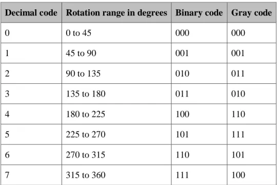
There are two popular types of absolute encoder: the gray and binary code encoders. From Figure 5, it can be seen that the main difference resides in the arrangement of dark and white spots. In the following, we consider a three-bit-digital-word absolute encoder; thus, we need three emitting diodes and three photo detectors mounted in parallel axes. The conversion from binary word to angle rotation is shown in Table 2.

(32)

Table 2. Three-bit digital word-to-angle conversion of an absolute encoder.

Decimal code Rotation range in degrees Binary code Gray code

0 0 to 45 000 000 1 45 to 90 001 001 2 90 to 135 010 011 3 135 to 180 011 010 4 180 to 225 100 110 5 225 to 270 101 111 6 270 to 315 110 101 7 315 to 360 111 100

For a three bit digital word, we get 23=8 angle rotations or distinct shaft positions. For a n-bit digital word, we have 2ndistinct angle rotations; thus, increasing the number of bits per digital word, significantly increases the precision of the position measurement. The gray code is preferred over the binary code since the uncertainty during one transition is always one bit.

2. Incremental Encoder

As shown in Figure 6 and Figure 7, the incremental or relative encoder has two sensors whose outputs are considered channels and called, respectively, channel A and channel B. The two output channels, A and B, are in quadrature, meaning they are 90 degrees out of phase. Waveforms A and B are decoded to produce a count-up pulse or a countdown pulse. Often, an additional output channel (INDEX) is added to count full revolutions. It is also used to define the zero position.

(33)

Example of channels A and B outputs (from [13]).

Incremental encoder (from [14]).

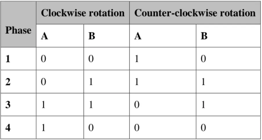
The principle of operation of an incremental encoder is illustrated in Table 3. For example, if the last value collected from A and B was 00 and the current value is 01, it means the wheel rotated a half step in the clockwise direction. Steps refer to the angle slots available on the wheel. By counting the number of steps the wheel rotated, we can determine precisely the position of the wheel at any time. The velocity can be determined from the angle of rotation and the time taken to perform the rotation. Generally, incremental encoders are preferred over absolute encoders since they give better results in term of precision and accuracy, with fewer electronic components involved.

(34)

Table 3. Example of output channels state diagram.

Phase

Clockwise rotation Counter-clockwise rotation

A B A B

1 0 0 1 0

2 0 1 1 1

3 1 1 0 1

4 1 0 0 0

B. OPTICAL MOUSE SENSORS

The idea of using optical mice as optical flow sensors is a powerful lure for robotics researchers due to several factors. First of all, mouse chips are capable of tracking 2D motions at very high resolutions. Second, they are small, light, and easy to mount on any robotics platform. Finally, the chips are abundant on the market and are inexpensive compared to the other optical flow sensors. The common problem of optical mouse sensors is that they are mainly designed to work on surfaces located a few millimeters from the sensor. Consequently, research was done to allow the application of these sensors where the platform or the robot is farther than a few millimeters from the tracking terrain. To accomplish this, optical imaging systems used in optical mice were modified with non-standard lenses, allowing the refocusing of light onto the sensor. The lenses used differ from one application to another according to the distance required between the sensor and the ground. Actually, this approach has been proven to work for different distances ranging from 2.0 cm above the surface for wheel-based robots to tens of meters for flying robots [15]–[16].

Three main factors need to be considered when selecting an optical mouse sensor for a certain application. These factors are the frame rate, the image size, and the resolution. The number of snapshots the sensor is capable of taking per second represents

(35)

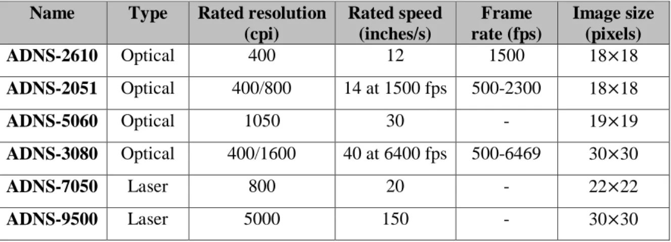
speed motion tracking also depends on the image size. That means if two sensors have the same frame rate, the one capable of taking larger images gives better results. For example, a 30 × 30-pixel-image sensor is better than an 18 × 18-pixel-image sensor. Finally, the last characteristic to consider in an optical mouse sensor is the resolution. The resolution of a sensor is usually expressed in counts per inch (cpi) and reflects the number of steps the sensor reports during a displacement of one inch. In other words, a high resolution sensor of 1600 cpi detects more surface details than a low resolution sensor of 400 cpi. The basic principles of operation for optical mice are described in detail in the next chapter as we introduce all the electronic components used to perform the experimental part of this thesis. The performances of different Avago-brand mouse chips are compared in Table 4.

Table 4. Characteristics of some Avago mouse-chip sensors.

Name Type Rated resolution (cpi) Rated speed (inches/s) Frame rate (fps) Image size (pixels) ADNS-2610 Optical 400 12 1500 18×18 ADNS-2051 Optical 400/800 14 at 1500 fps 500-2300 18×18 ADNS-5060 Optical 1050 30 - 19×19 ADNS-3080 Optical 400/1600 40 at 6400 fps 500-6469 30×30 ADNS-7050 Laser 800 20 - 22×22 ADNS-9500 Laser 5000 150 - 30×30 C. MOTION TRACKING

In robotics, three main reference frames are used to translate the motion of an object within a specific space. The first is the world frame, referred to as W frame. The second is the robot frame, referred to as R frame. The final one is the sensor frame, referred to as S frame. It is important to consider that the number of S frames depends on the number of sensors used since every sensor has its own frame. Let us consider the configuration of frames shown in Figure 8.

(36)

Example of reference frames configuration.

At the beginning, or at t=0, the W and R frames coincide. This means that the sensor and robot positions relative to the W frame are, respectively,

0 0 ; 0 0 0 W R W S S S R O O d O         = =_ _ =_{ }     _{ }   . (19)

As the robot moves, the position of the robot frame and sensor frame relative to the absolute frame change. Using rotation matrices and homogeneous transformations, we

(37)

can represent all possible motion of the robot with respect to the W frame. The rotation matrix of frame R relative to frame W is given by

cos( ) sin( ) 0 sin( ) cos( ) 0 0 0 1 W R R θ θ θ θ −     =       . (20)

Also, the rotation matrix of frame S relative to frame R is given by

1 0 0 0 1 0 0 0 1 R SR I     =_ _=     . (21)

The robot position represented in the W frame system can be written as cos( ) sin( ) 0 R W R R d O d α α     =       , (22)

and the sensor position represented in the R frame system can be written as 0 0 R S S O d     =       . (23)

Using the different rotation matrix and positions of frames relative to each other, we get the corresponding homogeneous transformations

cos( ) sin( ) 0 cos( ) sin( ) cos( ) 0 sin( ) 0 0 1 0 0 0 1 R W W R W R R R d d R O T θ θ α θ θ α −   =_ _=   0 0 0 0 1             (24) and 1 0 0 0 0 1 0 0 0 1 0 0 0 0 1 0 R R S R S S S d R O T =_ _=   0 0 1             . (25)

(38)

1 1 R W W W R W S S R R O O P= T × P= T × _   _{ }= _    , (26)

which can be written

cos( ) sin( ) 0 cos( ) sin( ) cos( ) 0 sin( ) 0 0 1 0 0 0 0 R R W W R R d d P T P θ θ α θ θ α − = × = 0 0 1 1 S d           _×               . (27)

Now, the sensor’s position coordinates relative to the world frame are

sin( ) cos( ) cos( ) sin( ) 0 S R W S S R d d x O y d d z θ α θ α − +         =_{ }=_ + _         . (28)

For each single motion of the robot (translation or rotation) we must solve these equations to know the position of the robot. With only two equations and three unknowns, it is difficult to determine the position of the robot. That is why, usually, multiple sensors are mounted on a moving platform. With only one sensor, dead reckoning is a complex problem to solve in robotics. In the next chapter, we present our solution that not only makes dead reckoning and odometry with only one sensor possible, but also remove the complexity of jumping from one frame to another by directly representing the position of the robot in the W frame.

(39)

(40)

IV. EXPERIMENTAL SETUP AND RESULTS

The main goal of this work is the design and development of an efficient, inexpensive, reliable, and simple obstacle avoidance and dead reckoning optical flow sensor that can be used in varying light conditions. All the steps taken to make this work achievable are outlined in this chapter. The work done throughout this thesis involved commercially available components, C++ coding, and custom algorithms. The components used to realize the experimental part of this thesis are the ADNS-3080, the Arduino Due, a DC motor board connected to four motors, a Parallax servo motor, and two XBEE modules.

A. HIGH PERFORMANCE OPTICAL MOUSE SENSOR ADNS-3080

The ADNS-3080 belongs to the family of ADNS optical mouse sensors manufactured by Avago Technologies. It is considered to be a high performance optical flow mouse sensor due to its key features that include the following [17]:

• Up to 40-inches per second (ips) and 15-g speed motion detection

• 500 to 6469-frames per second (fps) programmable frame rate

• 400 or 1600-counts per inch (cpi) selectable resolution

• 30 × 30 pixels image size

Accessing the sensor for data communication is possible through a four-wire Serial Peripheral Interface (SPI). The ADNS-3080 consists of an Image Acquisition System (IAS), a Digital Signal Processor (DSP), and a serial port. The IAS includes a tiny camera, a lens, and an illumination system. The DSP processes the microscopic terrain images captured by the IAS and determines the distance, the direction, and the Δx and Δy relative displacements. An external microcontroller can be used to access (read/write) the different registers of the sensor by using the SPI. The block diagram and pinout of the ADNS-3080 are shown in Figures 9 and 10, respectively.

(41)

Block Diagram of ADNS-3080 (from [17]).

Pinout of ADNS-3080 (from [17]).

The SPI is a synchronous serial port used to read the data from the different registers of the sensor or to select specific parameters such as resolution. To activate the serial connection, NPD must be set to high, RESET to low, and NCS to low. If NCS goes high during a transaction, the transaction is aborted and the SPI is deactivated. The clock input (SCLK) is always generated by the microcontroller. If multiple sensors are

(42)

connected to the same master, the NCS can be used to select one sensor and deselect the other. Every register in the ADNS-3080 has a unique address. The different registers and reset values are illustrated in Figure 11.

(43)

Understanding write and read operations is crucial to understanding how to exchange data between the microcontroller and the sensor. Write operations consist of two bytes both sent by the master over the master-out-slave-in line (MOSI): one byte for the address and one byte for the data. The first byte containing the address has “1” as its most-significant bit (MSB). The second byte containing the data is read by the sensor on SCLK rising edges. Similarly, read operations consist of two bytes. The address byte has “0” as its MSB and is sent by the microcontroller over MOSI. The data byte is driven by the sensor over the master-in-slave-out line (MISO). The sensor reads MOSI bits on every SCLK rising edge and delivers MISO bits on falling edges of SCLK. Minimum timing between two subsequent operations needs to be respected. The time window to be respected between two back-to-back operations is depicted in Figure 12.

Timing between subsequent operations (from [17]).

The ADNS-3080 has an 8-bit unsigned integer unique ID contained in the “Product_ID” register. The value contained in this register is always the same and is

(44)

usually read to make sure that the connection between the microcontroller and the sensor is functional. The “Revision_ID” register can also be used to identify the sensor’s version. Both the “Product_ID” and the “Revision_ID” registers are read only registers. The data, address, and reset values of the “Product_ID” and “Revision_ID” registers are illustrated in Figure 13.

“Product_ID” and “Revision_ID” registers (from [17]).

The “Motion” register contains information about the sensor motion and resolution. If motion has occurred since the last time the register was read, the MSB is set to “1”; otherwise, it is set to “0.” The least-significant bit (LSB) allows the user to know the sensor resolution setting. If it is “0,” the resolution is 400 cpi (default value). If it is “1,” the resolution is 1600 cpi. Once a motion has been detected, the user needs to read the “Delta_X” and “Delta_Y” registers to determine the relative displacements Δx and Δy, respectively. The “Motion,” “Delta_X,” and “Delta_Y” registers are all read-only registers. To set the sensor resolution to 1600 cpi, the user needs to access the “Configuration_bits” register and set the RES bit to “1.” The data and reset value of the “Motion,” “Delta_X,” “Delta_Y,” and “Configuration_bits” registers are shown in Figures 14, 15, and 16, respectiveley.

(45)

“Motion” register (from [17]).

(46)

“Configuration_bits” register (from [17]).

As an optical flow sensor, the ADNS-3080 must be able to operate with a large number of valid features visible in an image or frame; thus, a surface quality “SQUAL” register has to be regularly checked to make sure that the sensor is working properly. The surface quality factor provides an accuracy indication of the relative displacements computed by the sensor. A low “SQUAL” value makes the data collected and computed by the sensor unreliable. The quality factor is directly related to the navigation surface. The “SQUAL” is maximized when the distance between the navigation surface and the imaging lens is optimized. The “SQUAL” register data and reset values are illustrated in Figure 17.

“SQUAL” register (from [17]).

An imaging lens can significantly increase the maximum tracking speed. It provides a magnification factor equal to the rated tracking speed of the sensor divided by the desired speed. The magnification factor is also given by m=Si/So where Si is the

image distance and So is the object distance. From Figure 18, it can be seen that Si is the

(47)

Focal length, object distance, and image distance (from [18]).

In other words, a 1/m wide surface patch will be focused onto a 1 mm wide image plane within the ADNS-3080. The focal length of the lens can be expressed, according to [19], as

1 1 1 1 1 1 1

/

o i o o i i

f = S +S =S +mS = S m+S . (29)

Solving for So and Si, we get

1 (1 ) o f S f f m m = + = + (30) and (1 ) i S = +f mf = f +m . (31)

By knowing the focal length of an imaging lens, the magnification ratio can be set so that the surface quality factor is maximized and the size of the surface focused onto the camera’s image plane increased.

(48)

B. DC MOTOR SHIELD

A DC Motor Shield is used to control the speed and the direction of rotation of the wheels mounted to the indoor ground robot. The motor shield uses an H-bridge driver chip L298N integrated circuit that can drive up to two brushed DC motors or a four-wire two phase stepper motor. Each motor can be driven backwards or forwards. The speed of each motor is controlled by high quality, built-in pulse-width Modulated (PWM) signals generated by the microcontroller. The hardware diagram of the DC control board is shown in Figure 19.

DC Motor Shield parts (from [20]).

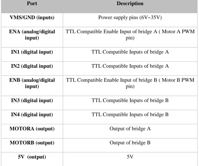
To power the board, an external power supply is needed. The input voltage ranges from 6 to 35 volts. All the ports and pins available in the board are listed in Table 5. Motor A is controlled via ports IN1, IN2, and ENA. IN1 and IN2 are used to control the direction of rotation. When IN1 goes high and IN2 goes low, motor A rotates clockwise.

(49)

clockwise. ENA is connected to a PWM port of the microcontroller to control the speed of the motor. The same applies for motor B on the IN3, IN4, and ENB ports.

Table 5. DC Motor Shield ports.

Port Description

VMS/GND (inputs) Power supply pins (6V~35V)

ENA (analog/digital input)

TTL Compatible Enable Input of bridge A ( Motor A PWM pin)

IN1 (digital input) TTL Compatible Inputs of bridge A

IN2 (digital input) TTL Compatible Inputs of bridge A

ENB (analog/digital input)

TTL Compatible Enable Input of bridge B ( Motor B PWM pin)

IN3 (digital input) TTL Compatible Inputs of bridge B

IN4 (digital input) TTL Compatible Inputs of bridge B

MOTORA (output) Output of bridge A

MOTORB (output) Output of bridge B

5V (output) 5V

C. ARDUINO DUE

Arduino is an open-source physical computing platform that can be used to collect information from several sensors and control a variety of actuators, motors, lights, or other peripherals. All of the collection and control processes are controlled from a single thread of execution in the microcontroller. Arduino provides the user with different microcontroller boards that can be purchased preassembled or as do-it-yourself kits. Arduino is a simplified entry point to create and build digital devices and interactive

(50)

objects capable of sensing and controlling the physical world. Arduino also provides the user with an Integrated Development Environment (IDE) that supports C and C++ programming languages. The IDE is a clear and simple programming environment used to write programs for the Arduino board. Also, the IDE gives the opportunity to check the code for possible errors before uploading it to the microcontroller. The Arduino IDE software runs on Windows, Macintosh OSX, and Linux operating systems.

Most of the Arduino boards run at 5.0 volts, except the Arduino Due which runs at 3.3 volts. The ADNS-3080 and the XBEE pro 90 modules both run at 3.3 volts. That means the maximum voltage that the I/O pins can tolerate is 3.3 volts. Forcing the optical mouse sensor or the transceiver module to operate at 5.0 volts can damage them. To avoid any possible incident, the Arduino Due was selected for our work. The Arduino Due front and back sides are displayed in Figure 20.

Arduino Due Board (from [21]).

The Arduino Due board contains a 32-bit Atmel SAM3X8E-ARM processor. It has 12 analog inputs and 54 digital input/output pins. Twelve of the digital input/output pins can be used as PWM outputs. The Arduino Due also has a SPI to communicate with another microcontroller or one or more peripheral devices. MISO, MOSI, and SCLK lines are common for all devices. The chip-select or slave-select (SS) line is specific for every device. The microcontroller board operates at 84 MHz clock speed. It has two digital-to-analog converters (DACs), a reset, and an erase button. The Arduino Due

(51)

Arduino Due ports (from [21]).

In this work, only one Arduino Due board was used. All the data traffic and control signals were managed by the microcontroller. The Arduino Due is the master and all the other parts of the ground robot (ADNS-3080 modules, XBEE pro 90, DC Motor Shield, and Parallax servo) were slaves.

D. PARALLAX STANDARD SERVO

The Parallax Standard Servo (see Figure 22) is designed to hold any position between 0 and 180 degrees. It is a high precision servo that can be controlled by a microcontroller or device capable of generating PWM signals. From Figure 23, it can be seen that the connection of the servo to any type of microcontroller is easy to realize.

(52)

Parallax Standard Servo (from [22]).

Parallax Standard Servo Wiring Diagram (from [22]).

The position of the servo shaft is directly controlled by the width of the PWM signal pulses. The servo needs a period of 20.0 ms between pulses to hold its position. To center the servo, the microcontroller must deliver a 1.5 ms pulse every 20.0 ms. The PWM signal required for a centered servo is shown in Figure 24.

(53)

The pulse duration ranges from 0.75 to 2.25 ms. A 0.75 ms pulse corresponds to the servo shaft positioned at 0 degree. A 2.25 ms pulse corresponds to a servo shaft position of 180 degrees. The center position corresponds to a servo shaft position of 90 degrees. So, depending on the pulse duration, the servo shaft can rotate either clockwise or counter-clockwise.

E. XBEE-PRO 900 DIGIMESH RF MODULES

The XBee-PRO 900 RF modules (see Figure 25) were mainly engineered and designed to be used in wireless sensor networks (WSNs). They are reliable and require low power to operate efficiently. They operate within the ISM (industrial, scientific, and medical) 900-MHz frequency band to support up to 10 km (using high gain antennas) RF line-of-sight ranges and 156 kbps data rates.

XBee-PRO 900 DigiMesh RF module (from [23]).

The XBee-PRO 900 can communicate with any host that has a Universal Asynchronous Receiver/Transmitter (UART) interface. At the source, the UART converts parallel-form data into serial-form data. At the destination, the UART receives the bits of data and reassembles them into bytes of data. Any microcontroller supporting a UART interface can be directly connected to the pins of the RF module. From Figure 26, it can be seen that the UART system data flow diagram is based on a four-wire connection. RTS and CTS pins correspond, respectively, to Request-to-Send and Clear-to-Send pin flow control pins.

(54)

UART Data Flow Diagram (from [23]).

F. TRAJECTORY-FOLLOWER ROBOT

The idea of the trajectory-follower robot came from the principle of operation of the Flight Management System (FMS) in aircraft. The FMS is an embedded system that keeps track of the aircraft’s position by collecting data from its various sensors (GPS, INS, radio navigation tools, etc.). The FMS consists essentially of a Flight Management Computer (FMC) connected to the different sensors and a Control Display Unit (CDU). Before take-off, a flight plan is entered by the pilot via the CDU into the FMS. The flight plan is the route the aircraft must follow to fly from the departure point to the destination point and contains all the waypoints needed to reach the destination. Once in flight, knowing the aircraft’s position and the flight plan, the FMS can guide the aircraft along the way by controlling the autopilot and the auto-throttle systems. The different parts of a typical FMS are displayed in Figure 27.

(55)

Example of a typical FMS (from [24]).

In this work, the Arduino Due plays the role of the FMC. A desktop computer plays the role of the CDU, and the DC motor board plays the role of the autopilot and auto-throttle systems. Using the Arduino IDE installed in the control unit, we uploaded the program containing the different waypoints to the microcontroller. Once the program was uploaded, the processor collects position information from the ADNS-3080 optical mouse sensor. Given the robot position and route plan, the Arduino Due controls the speed and direction of rotation of the wheels via the DC motor board. The position information and the robot maneuvers are displayed on a display unit located in a monitoring area. The control unit and the display unit can be located at the same place. An RF connection between the display unit and the onboard computer is established by using two XBee-PRO 900 modules. The emitter module is mounted to the robot and directly connected to the microcontroller via one of its four UART interfaces. The receiver module is directly connected to the display unit via the serial port. The different parts of the wheeled-robot’s onboard system are shown in Figure 28.

(56)

Indoor robot embedded system.

This work involved extensive coding and programming. Every component had to be programmed and tested separately, and all the resulting codes had to be combined into one final program. The resulting program allowed the microcontroller to read and edit the data contained in the different registers of the optical flow sensor, control the speed and direction of rotation for the motors, and continuously send information of position and behavior to the display unit. The master can access all the registers of the ADNS-3080 chip. To track the robot’s position, the microcontroller initializes the sensor, configures its settings, and collects position data from all the registers involved in the dead reckoning process. All the useful data are sent out to the display unit via the RF link. Getting a surface quality feedback from the sensor is very important since a high quality

(57)

ability to reliably track position improves. A significant drop in the quality factor indicates that the dead reckoning process is no longer reliable.

Communication protocol between the Arduino Due and the ADNS-3080 sensor.

(58)

The communication process between the microcontroller and the optical mouse sensor is described by the flowchart presented in Figure 29.

As said before, traditional techniques of dead reckoning using data collected and measured by encoders attached to either the robot’s wheels or the engine axis suffer from slipping and crawling. Slipping occurs when wheels slide, and crawling occurs when an external force is exerted on the robot. The dead reckoning we propose here is slipping and crawling resistant since the position tracking function is attributed to one ADNS-3080 sensor. The mouse sensor is not bound to any moving part and is capable of reading relative displacements even when an external force is behind the robot movement. Accurate dead reckoning using optical flow sensors usually involves the use of more than one sensor due to the fact that a robot change of direction is hard to measure using only one sensor. In some works, two optical mouse sensors have been used. In others, arrays of optical mouse sensors have been utilized. Indeed, the use of only one optical flow sensor for dead reckoning may seem like a bad idea unless the robot is also equipped with one or multiple other heading sensors. A novel and efficient mean of using one optical mouse sensor pointed at the ground as a heading and dead reckoning sensor is presented in this work.

The first thing we must consider when using a two or four-wheeled robot is how to make a right or a left turn. A common technique is to vary the speed of the wheels. For instance, if the left wheels rotate faster than the right wheels, the vehicle moves to the right, and vice versa. The distance required to make a turn depends directly on how slowly the left (right) wheels spin and how quickly the right (left) wheels spin. With only one optical mouse sensor, this scenario is not appropriate since the robot position changes continuously during the turn; thus, the position tracking process cannot be reliable.

In this work, we opted for another technique to reduce the complexity associated with the above method. In order to make a turn, the right and left wheels rotate at the same speed but in opposite directions. For example, when the right wheels rotate forward and the left wheels rotate backward, the robot makes a left turn. Contrarily, when the

(59)

occurs. In other words, a right or left turn causes only the robot to spin about its ZR-axis. An example of a right turn is illustrated in Figure 30. As we can see, the position of the robot remains unchanged; however, after the manoeuver, the robot points θ degrees to the right.

Right turn of θ degrees.

Similar to an aircraft equipped with an FMS, the trajectory-follower robot needs to move from one point to another. Given the robot’s current position and the next waypoint, the onboard computer has to compute the route to follow in order to reach the next destination and then compute the necessary commands to be executed by the motor system. The problem to solve is how to compute and track a change in direction. In this work, after attempting several methods, we determined how to accomplish this using the same sensor, and there is no need to add an additional payload to the platform. When a turn is being executed, only a change in the relative displacement Δx is detected. No changes in the relative displacement Δy occur. The change relative to the x axis corresponds to an arc of length

(60)

pos

x = ×θ R. (32)

For example, a 90-degree right or left turn corresponds to an x-displacement of ± R × π/2. The different phases required to execute a 45 degree right turn are listed in the following flowchart (Figure 31).

Example of right turn.

The turn speed and direction depend directly on the command signals sent out by the onboard computer to the DC motor board. Given the robot type, the DC motor board can be connected to either two or four DC motors. The wheels are directly mounted to the DC motors. To move from one point to another, the microcontroller needs to first determine the direction and then the distance required to reach the next destination. Every time the robot reaches one waypoint, new computations need to be done. Once done with

(61)

translate the data computed into displacement. Meanwhile, the Arduino Due also collects position information from the dead-reckoning sensor. Every time a destination is reached, the robot stops for a period of few seconds to give the microcontroller enough time to calculate the next set of instructions. Consider the example shown in Figure 32. If the robot is to go from point (xk,yk) to point (xk+1,yk+1), the heading angle and the distance to target are, respectively,

(

)

(

1

)

1 1 tan k k k k x x y y θ − + +  −  =   −     (33) and

(

) (

2

)

2 1 1 k k k k D= x ₊ −x + y ₊ −y . (34)

Example of heading and distance to target computation.

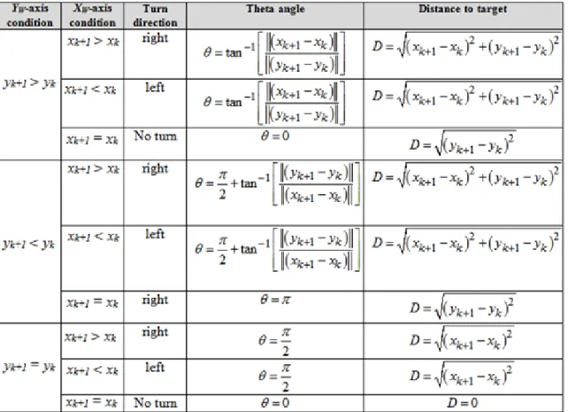
The θ and D values calculated above are not valid for all scenarios. Depending on the position of one point with respect to the previous one, we see that the heading angle and distance to target values may vary. From Table 6, we conclude that there are nine possible scenarios.

(62)

Table 6. Theta angle and distance to target for all possible scenarios.

With all cases addressed for calculating the heading and distance, we now discuss the algorithm adopted and executed by the trajectory-follower robot. At time t=0, the world frame and the robot frame coincide. All the robot positions are only relative to the world frame. Note that at every waypoint, the robot has to make a θ-turn in the direction opposite to the initial one he made to reach that point. Before every new computation of heading and distance to target, the robot frame x- and y-axis are, respectively, oriented the same way as the world frame x- and y-axis. An example of four-waypoint trajectory is illustrated in Figure 33.

(63)

Example of four-waypoint trajectory.

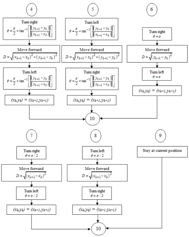
The behavior of the trajectory-follower robot is explained in more detail in the flowchart presented in Figure 34. The flowchart considers all possible scenarios.

(64)

Principle of operation of the trajectory-follower robot (continued on next page).

(65)

Figure 34. Principle of operation of the trajectory-follower robot (continued from previous page).