Adjustability of a discrete particle swarm optimization for the dynamic TSP

Title: Adjustability of a discrete particle swarm optimization for the dynamic TSP

Author:

Łukasz Strąk, Rafał Skinderowicz, Urszula Boryczka

Citation style:

Strąk Łukasz, Skinderowicz Rafał, Boryczka Urszula. (201

8).

Adjustability of a discrete particle swarm optimization for the dynamic TSP. "Soft

Computing" (Vol. 22 (2018) s. 7633–7648), doi 10.1007/s00500-017-2738-9

https://doi.org/10.1007/s00500-017-2738-9

M E T H O D O L O G I E S A N D A P P L I C AT I O N

Adjustability of a discrete particle swarm optimization

for the dynamic TSP

Łukasz Str ˛ak1 · Rafał Skinderowicz1 · Urszula Boryczka1

Published online: 28 July 2017

© The Author(s) 2017. This article is an open access publication

Abstract This paper presents a detailed study of the dis-crete particle swarm optimization algorithm (DPSO) applied to solve the dynamic traveling salesman problem which has many practical applications in planning, logistics and chip manufacturing. The dynamic version is especially important in practical applications in which new circumstances, e.g., a traffic jam or a machine failure, could force changes to the problem specification. The DPSO algorithm was enriched with a pheromone memory which is used to guide the search process similarly to the ant colony optimization algorithm. The paper extends our previous work on the DPSO algorithm in various ways. Firstly, the performance of the algorithm is thoroughly tested on a set of newly generated DTSP instances which differ in the number and the size of the changes. Secondly, the impact of the pheromone memory on the con-vergence of the DPSO is investigated and compared with the version without a pheromone memory. Moreover, the results are compared with two ant colony optimization algo-rithms, namely theMAX–MIN ant system (MMAS) and the population-based ant colony optimization (PACO). The results show that the DPSO is able to find high-quality solu-tions to the DTSP and its performance is competitive with the performance of the MMAS and the PACO algorithms. Moreover, the pheromone memory has a positive impact on

Communicated by V. Loia.

B

1 _{Institute of Computer Science, University of Silesia in}

Katowice, B¸edzi´nska 39, 41-205 Sosnowiec, Poland

the convergence of the algorithm, especially in the face of dynamic changes to the problem’s definition.

Keywords Discrete particle swarm optimization · Pheromone memory·Dynamic traveling salesman problem· Population-based ant colony optimization

1 Introduction

A problem in which input data are variable (i.e., time depen-dent) is called a dynamic optimization problem (DOP). The aim of optimization in the DOP is to continuously track and adapt to changes and quickly find the best solution (Li 2011). DOPs can be divided into two groups (Mori and Kita 2000):

online(direct adaptation) andoffline(indirect adaptation). In the first case, the changes are hard to predict and could happen at any moment during the algorithm runtime. In the sec-ond case, the changes happen at specified intervals between which the problem definition does not change. Many other DOPs classification criteria were described byYang and Yao (2013), including

– time linkage— is the change affected by the current solu-tion;

– cyclicity—is the change to the problem cyclic or not; – factors—do the changes affect the number or values of

variables, constraints, etc.

DOPs were investigated mostly in the context of the continu-ous optimization. In this work, we focus on the discrete DOP that is the DTSP in theofflineversion.

Computational intelligence methods are a set of tech-niques that are used to solve optimization problems. They include algorithms that were inspired by the collective

behav-ior of animals which are able to solve complex problems in their natural environment by cooperating with one another. It is often beyond the capabilities of a single individual to solve these problems, i.e., to accomplish tasks such as forag-ing and nest buildforag-ing, yet this is not problematic for a group of animals. When a combination of relatively simple behav-iors of particular individuals produces complex interactions, then we can talk about swarm or collective intelligence.

The PSO is a good example of a computational intelli-gence algorithm inspired by the natural behavior of animal herds, e.g., a school of fish or a flock of birds. Both fish and birds are able to coordinate the movement of the flock with-out the need to communicate directly. The PSO was proposed byKennedy and Eberhart(1995) in order to solve the func-tion optimizafunc-tion problem. In the PSO, a swarm (populafunc-tion) of particles moves around in the solution search space. Each particle has a position that corresponds to a solution to the problem being solved and velocity that shows the direction and velocity of the movement. A movement of a particle is also influenced by its local best known position, typically denoted byp Best, and the best position found by the swarm (usually denoted byg Best). This indirect interaction of the particles is intended to guide the swarm toward solutions of good quality. The relative simplicity and efficiency of the PSO was a key to its many successful applications, also in solving the discrete combinatorial optimization problems.

The behavior of certain species of ants that forage for food provided inspiration for creating ant colony algo-rithms (Dorigo and Stützle 2010). While searching for food, these ants lay a certain amount of pheromone as they move. At the beginning, they randomly choose the direction of the search process. With each subsequent trip from the nest to a food source and back, over time ants will deposit the largest amount of pheromone on the shortest path because much of the pheromone that has been laid on longer paths will evapo-rate before being reinforced by returning ants. After a while, a given pheromone trail will be reinforced to such an extent that when beginning its trip, each subsequent ant will follow that pheromone trail that has been laid down on the shortest path from the nest to a food source. In this case, pheromone acts as a means of indirect communication and in a way as

collective memory. Ant colony algorithms and particle swarm optimization are the most popular methods that were inspired by natural collective animals behavior.

It is easy to compare two algorithms based on compu-tational experiments if these algorithms can be run on the same input data. As for the traveling salesman problem, the TSPLIB library facilitates such comparisons (Reinelt 1995). Apart from data themselves, this library also provides opti-mal solutions for most problems. However, there is no such library for the dynamic traveling salesman problem. One of the aims of this paper is to create a new approach for test-ing the quality of results that are obtained for the DTSP.

A library of the DTSP instances that have been generated contains information about optimal solutions for every sub-problem which allows for a simple and precise evaluation of the performance of the algorithms. This library was used to compare the swarm intelligence algorithms investigated in this paper, i.e., the DPSO, the MMAS and the PACO.

1.1 Contributions

Compared to our previous articles on the DPSO for the DTSP (described briefly in Sect. 2), the research has been extended in a few directions. Firstly, we closely compare the convergence and efficiency of the two DPSO versions: the DPSOR−, in which the pheromone values are preserved between the subsequent modifications of the input data (prob-lem) changes, and the DPSOR+, in which the pheromone is reset after each change. Secondly, we introduce a systematic way of generating new DTSP instances (a DTSP instances generator), which allows to precisely control the number and range of the changes. Thirdly, based on the newly gener-ated DTSP instances, we investigate how the performance of the DPSOR+ and DPSOR−changes depending on the number of dynamic changes to the problem being solved. Lastly, based on statistical analysis, we compare the perfor-mance of the DPSO algorithms with the MMAS and PACO algorithms that were proven to perform competitively when solving many static and dynamic combinatorial optimization problems, including the TSP and DTSP.

The structure of this paper is as follows: The second sec-tion presents a review of literature on the dynamic traveling salesman problem and discrete particle swarm optimization algorithm. The third section describes the DTSP, whereas the fourth section contains a description of the tested algorithms that solve the DTSP. The tests that were carried out are pre-sented in the fifth section, and the final section presents a summary and conclusions.

2 Related work

The dynamic traveling salesman problem was first described by Psaraftis (1988). This problem is based on a change in both the number of vertices and a distance matrix that occurs over time. Each change can modify the optimal route, and the knowledge of the optimum is useful to be able to mon-itor the quality of the results that are being produced by an algorithm. Younes et al. (2003) proposed a procedure in which the optimal route does not have to be known for each subproblem. A modification is carried out for half the num-ber of subproblems (adding, removing or changing a given distance), and each of these changes is undone in the sec-ond half of the procedure. Data are the same in the first and the last subproblem. The algorithm is run for each

subprob-lem, but distances are only compared against the optimum for the last subproblem. Another approach combines static data with data obtained from satellites orbiting the Earth. Satellite orbits are given by a formula and the optimal route only changes within these orbits (Kang et al. 2004). Unfor-tunately, the dynamics of this problem is low; for example, the CHN146 + 3 problem contains 146 cities and 3 variable points. Yet another approach involves estimating the optimal value. In order to do this, one can use the Held–Karp algo-rithm that is based on the concept of 1-tree. This approach was adapted inBoryczka and Stra˛k(2013). An advantage of taking this approach is that one can quickly estimate the opti-mal value, whereas its greatest drawback is that there is no approximation error margin. However, an improved method which was proposed byHelsgaun(2000) allows one to esti-mate the optimum length with an error of less than 1%, but cannot predict what the results will be for other instances. Another method was proposed byGuntsch et al.(2001) when solving the DTSP with the ACO. The approach involves sim-ulating dynamic changes to the problem by exchanging a number of cities between the current problem instance and a spare pool of cities. As the method affects the optimum, Guntsch et al.(2001) evaluated their algorithms based on the relative differences in the length of the successive solutions. A more general method for generating dynamic versions of combinatorial optimization problems (COPs), including the TSP, was proposed byYounes et al.(2005). The basic idea, in the context of genetic algorithms, exploits the fact that most optimization methods involve some form of mapping from the problem solution space to the individuals used in the algorithm, e.g., a permutation of nodes. To simulate dynamic changes to the problem, the mapping function is modified by exchanging labels (indices) of some nodes; thus, the individuals represent different solutions, but the fitness land-scape, and so the optimum, of the problem instance does not change.Mavrovouniotis et al.(2012) proposed a more flexi-ble approach in which the encoding of the proflexi-blem instance is modified, instead of the encoding of the individuals. In the case of the TSP and VRP, it involves swapping the loca-tions of pairs of nodes. The method keeps the optimum intact and allows for precise control over the number of dynamic changes to the problem instance. However, this approach does not necessarily reflect each real-world scenario.

The PSO algorithm has been adapted several times to solve the TSP. The first version of the DPSO was proposed byHu et al.(2004). All particles were coded as binary strings. The predefined velocity was interpreted as the probability of a bit state transition from zero to one and from one to zero, but a sigmoid function could be used to restrict the values to 0 and 1. Zhong et al.(1997) proposed a new algorithm for the TSP in which the position of the particle was not a permutation of numbers but a set of edges. It used the parameterc3, named

by the authors a mutation factor, which allowed control the

balance between the exploration and the exploration in a dis-crete search space. Descriptions of the most PSO algorithms for solving the TSP can be found, together with the results, inGoldbarg et al. (2008). A hybrid of the PSO algorithm and pheromone was used inKalivarapu et al.(2009). This approach was implemented to deal with the problem of opti-mizing a function in a continuous space. The survey of the PSO approaches to the dynamic continuous optimization can be found inBlackwell et al.(2008).

There are relatively few applications of the DPSO in the realm of dynamic COPs.Okulewicz and Ma´ndziuk (2013) proposed a two-phase PSO to solve the dynamic VRP. In the first phase, the PSO was responsible for the assignment of the customers to vehicles, while in the second phase sep-arate instances of the PSO were used to find the order in which the customers should have to be visited (static TSP). A similar approach was proposed inDemirta¸s et al.(2015). Khouadjia et al.(2010) proposed an adaptive PSO for solv-ing the VRP with dynamic requests. The algorithm stored previous solutions in the form of a memory continuously updated during the algorithm runtime. The old solutions in the memory were used as starting points when a change to the problem definition was detected, as the changes could result in a new optimum being in the vicinity of the old one. A recent thorough survey on swarm intelligence methods for solving the dynamic COPs (continuous and discrete) can be found inMavrovouniotis et al.(2017).

The literature on the DPSO algorithm for the DTSP is very limited. This paper constitutes an extension of our ear-lier work on the DPSO algorithm. The initial version of the DPSO algorithm was presented inBoryczka and Stra˛k(2012) andBoryczka and Stra˛k(2013). That version differed from the one presented in this article in the pheromone update formula and the solution construction process. InBoryczka and Stra˛k (2015a), a new version of the DPSO algorithm was presented, in which the computations were reset based on the generated solutions entropy. The most recent work ofBoryczka and Stra˛k(2015b) concerned the problem of the automatic algorithm parameter values adaptation. In this arti-cle, we extend the previous work on the DTSP algorithm, as presented inBoryczka and Stra˛k(2015a,b), in several ways. Various solutions were proposed to adapt the ant colony algorithms, including the ACO and PACO, to solving the DTSP. One of the simplest ways of dealing with dynamic changes is to reset the pheromone memory after a change was detected; unfortunately, this strategy is not very effec-tive because it leads to the loss of all the information about the previous version of the problem that has been collected in the pheromone memory. Guntsch et al. compared a strategy that involves resetting the entire pheromone memory with two strategies of modifying the pheromone only in the neighbor-hood of a point where a change in the problem’s configuration has been detected; this modification involves adding or

removing a TSP node (Guntsch and Middendorf 2001). How-ever, strategies that involved resetting only a selected part of the pheromone matrix did not produce significantly bet-ter results than those obtained in the case of resetting the entire memory. The authors of the PACO algorithm tested its usefulness in solving the DTSP and QAP (Guntsch and Middendorf 2002). Another idea proposed in the literature was to diversify the ants population (Eyckelhof et al. 2002; Mavrovouniotis and Yang 2010;Boryczka and Stra˛k 2015a). After each change to the problem’s definition, the diversity of the ants population was increased to allow for a faster adapta-tion to the new version of the problem. In the recent years, the ACO algorithms were successfully applied to other dynamic combinatorial optimization problems. A good example is the dynamic generalized traveling salesman problem (DGTSP) for whichPintea et al.(2007) proposed an algorithm based on the ant colony system (ACS). The computational experi-ments on a set of the DGTSP instances, created based on the TSPLIB repository, confirmed efficiency of the suggested algorithm. A similar approach was also confirmed to be use-ful when solving the generalized vehicle routing problem (Pop et al. 2009). Time is a scarce resource when solving the dynamic combinatorial optimization problems; thus, paral-lel computations are very useful to accelerate the process of finding solutions to a new version of a problem, i.e., after a dynamic change. A parallel ACO was proposed inPintea et al.(2012) in order to solve the Euclidean DTSP instances with a few thousand nodes. A recent survey of the parallel ACO algorithms can be found inPedemonte et al.(2011).

3 Dynamic TSP

The classical TSP problem is typically modeled using a com-plete, weighted graphGdefined as follows:

G= V,E, w,

where:

V is a set of vertices representing cities,

V×V ⊂Eis a set of edges representing roads between cities;|E| =n₂,n= |V|(a complete graph),

wis a function of weights:E → R, ∀e∈ E,w(e)is the weight of an edge.

The problem involves finding the minimum Hamiltonian cycle in graph G, i.e., the shortest closed path that goes through all vertices exactly once. The problem that is ana-lyzed in this paper is symmetric: dab = dba (where di j

denotes the distance between citiesi,j) and Euclidean— any set of three cities,{a,b,c} ⊆ V, satisfies the triangle inequality:dac≤dab+dbc.

The DTSP formulation is an answer to many real-world scenarios, in which the external conditions alter the origi-nal definition of the static TSP. For example, the travel time between a pair of nodes may increase due to a higher traffic or a car accident. In another scenario, new customers (nodes) have to be accounted for or some of the current ones become unavailable. In our work, we assume that the changes to the problem definition are not very frequent.

The model of the DTSP consists of a sequence of modified static TSP subproblems, and every change in these subprob-lems means a modification of the distances and/or the number of vertices (Psaraftis 1988). In formal terms, this problem can be defined in the following way (Li et al. 2006):

D(t)= {di j(t)}n(t)×n(t), (1)

where:

tdenotes the parameter of time or the subproblem num-ber,

i, jdenote the ends of an edge,

n(t)denotes the number of vertices as a function of time. A change is made randomly and only with regard to a selected subset of vertices. Only the variant that involves a change in a distance matrix is analyzed in this paper.

3.1 DTSP Instances Generator

In the context of the DTSP, different algorithms are usu-ally compared in such a way that the coordinates of vertices (cities) are randomly modified for each execution of an algo-rithm; therefore, each time, the search space changes in a slightly different manner. The tests that were presented inBilu and Linial(2012) show that each change in the con-figuration of the problem entails a change in the location of the global optimum which is difficult to predict. It also has other consequences, such as a change in the problem’s difficulty level. The difficulty of the TSP can be analyzed in the context of, for example, the distances between local minima as well as between local minima and the global opti-mum. If the distance between the global optimum and the other optima is large, the search process can easily get stuck in a local optimum (Bilu and Linial 2012). Thus, the prob-lem’s difficulty increases in a way that is hard to predict. In order to facilitate a comparison between the analyzed algo-rithms in terms of efficiency in the context of the DTSP, the following strategy was adapted. A set of TSP instances was selected from the TSPLIB library (Reinelt 1995), on the basis of which instances of the DTSP were created (the TSPLIB format was maintained) by randomly changing the location of a predetermined number of vertices in accordance with Algorithm1. The resulting DTSP instance consisted of11

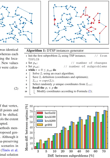
Fig. 1 On the left-hand side is a visualization of the optimal route for the problem (ch130), whereas on theright-hand side, the edges that differentiate the optimal solution that had been created before the changes were made from the one that was created after those changes are marked inred(color figure online)

consecutive subproblems; the first subproblem was identical to the TSP instance from the TSPLIB library, whereas each subsequent subproblem was created by changing the loca-tion of a predetermined proporloca-tion of vertices. New values of coordinates(p_x,p_y)of a given vertex (city) were calcu-lated in accordance with the formula:

r = fi n f ·r and(0,da_vg)

φ=r and(0,2π) p_x =px+r·cos(φ)

p_y =py+r·sin(φ),

(2)

where(px,py)denote the previous location of that vertex,

davgrepresents the average distance between all points and

φ stands for the angle at which the point will be shifted. Parameter fi n f is a scaling parameter that controls the extent

of changes; in this paper, a value of 0.3 was adapted. Compared to some of the more advanced methods men-tioned in Sect.2, the location changes in the proposed gen-erator influence the optima of the subproblems. Although it is clearly a disadvantage compared to the optima-preserving methods, it may be closer to many real-world scenarios in which weights of the TSP edges are modified (Tinós et al. 2014). For each subsequent subproblem, an optimal solution was determined by using the Concorde algorithm (Applegate et al. 2006).

Equation2 enables a precise control over the extent of changes to the DTSP definition. Moreover, it preserves the triangle inequality of the distances between the nodes; thus, the problem after a change should not be more difficult to solve than the original version. This makes it easier to focus on the behavior of the studied algorithms.

Figure1 shows the optimal solutions for two consecu-tive subproblems for theberlin52instance. The edges that differentiate the new solution from the previous one have been highlighted. The current library1contains 64 problems which are based on eight problems from the TSPLIB library:

berlin52,kroA100,ch130,kroA200,gil262,gr202,pcb442

andgr666; for each of them, a total of eight DTSP instances

1_{The library also contains charts presenting optimal solutions, and it}

can be made available upon request to the authors.

Algorithm 1:DTSP instances generator

1 Init the first subproblemI0using TSP instance; // from TSPLIB

2 Setpm; // number of changes

3 Setpsub; // number of subproblems

4 whilet=0≤psubdo

5 SolveItusing an exact algorithm;

6 SaveItdefinition (coordinates and optimum);

7 I_t+1=copy(I_t);

8 Select randomlypunique coordinates fromIt+1;

9 forall the pi∈pdo

10 Modify coordinates according to Formula (2);

Fig. 2 Mean difference between consecutive DTSP subproblems’ global optima as measured by the number of different (new) edges ver-sus the differences between consecutive subproblems (which is equal to the percent of the total number of vertices whose locations underwent a change)

have been generated, which differ in terms of the percent-age of vertices that undergo modifications. The following percentages were assumed: 3, 5, 10, 20, 30, 40, 50, 60 and 70%. For example, for a value of 5%, consecutive subprob-lems differ in terms of the coordinates0.05·nof vertices, wherendenotes the total number of vertices (problem size). Figure 2 shows how much the consecutive optima differ from one another in terms of the number of vertices that undergo changes. As can be seen, the greater the number of coordinates that undergo changes, the larger the differ-ences between the consecutive optima, and these differdiffer-ences

increase with the size of the problem. For example, if subse-quent subproblems are created for the problemkroA200by changing the location of 30% of vertices, then subsequent optimal solutions contain approximately 50% of new edges relative to the previous solution.

4 Particle Swarm Optimization

A pheromone is a characteristic component of ant colony algorithms, in which a set of ants lay virtual pheromone trails on elements of the search space (solution space). The clas-sical PSO algorithm does not use pheromone, but there are hybrid versions of this algorithm that do. This is true for both continuous and discrete optimization algorithms.

4.1 DPSO

Many concepts had to be redefined in order to adapt PSO algorithm to a discrete search space. The algorithm that was proposed inZhong et al.(1997) is based on sets of edges. A single edgeeis an ordered 3-tuple(a,x,y), wherea ∈ [0,1] denotes the probability of choosing this edge when moving to the next position andx,y∈V,∀x,yx=ydenote the ends of

that edge. In this algorithm, the solution to the TSP:{(1,2); (2,3); (3,4); (4,1)} takes the following form: {(1,1,2), (1,2,3),(1,3,4),(1,4,1)}. The position of particleXis rep-resented by a set of edges that constitute a Hamiltonian cycle. VelocityVrepresents the search direction. It is a set of edges that can contain a partial solution to the problem (it does not contain all the edges that are needed to create a Hamil-tonian cycle) or redundant edges. The common feature of all particle swarm optimization algorithms is that they work based on an equation that describes a particle’s movement in the search space. The original DPSO algorithm (Zhong et al. 1997) does not use pheromone which provides an adaptation mechanism for the DTSP. Formulas (3) and (4) present the authors’ own discrete version of these equations that take into account pheromone (firstly described inBoryczka and Stra˛k(2012)). V_ik+1=c2r and()·(g Best−Xik) +c1r and()·(p Besti−X_ik) +ω·V_ik (3) Xk_i+1=τk(V_ik+1) step a ⊕c3r and()·X_ik step b (4)

whereidenotes the particle number,k—the iteration number andr and()—a random variable within the range[0,1]. The sets of edgespBestandgBestrepresent particlei’s best posi-tion and the best soluposi-tion that has been found, the addiposi-tion

and subtraction operators denote the sum and difference of the sets, and coefficientωis called the inertia weight. Param-etersc1andc2are cognitive and social scaling coefficients,

respectively; they assign the appropriate values to parame-terafor each element of thepBestandgBestsets. Operator

⊕adds the missing edges to the next position; these edges are necessary for creating the correct route for the TSP. For this purpose, the operator uses the edges that were used to calculate the previous position. The way in which the opera-tor works will be explained later in this paper. The function τk _{increases the probability of going to the next position}

by using pheromone which has already been employed in ant colony algorithms. The function is used in row 10. Algo-rithm2 for calculating a particle’s next velocity as well as at the stage of edge filtering. The reinforcement function is given by formula: τk₍ V_ik+1)=a+ [(τx y−0.5)· k pi t ], ∀(a,x,y)∈V_ik+1⊆E (5)

where (a,x,y)denotes an edge that belongs to the set of velocities, τx y represents the value of pheromone that has

been read from the pheromone matrix,kstands for the algo-rithm iteration number and pi t denotes the number of all

iterations of the algorithm. Coefficient _pk

i t is a scaling coef-ficient that controls the strength of (positive or negative) reinforcement based on the number of iterations of the algo-rithm that have been carried out. As a result of executing function (5), a set of edges is created with coefficienta(i.e., the probability of using a given edge to go to the next position) which has been positively or negatively reinforced. The value of the reinforcement is within the range [−0.5,0.5]. The pheromone that has been assigned a negative value (repel-lent) is interpreted as a penalty function which repels those edges that do not improve the quality of the obtained solution. In this way, the algorithm only chooses those edges that have a high chance of being a part of good quality solutions as rep-resenting a given particle’s next position. Uncertainty about the quality of edges is reflected in the pheromone value. The higher the value, the more probable it is that a given edge will improve the solution. In subsequent iterations of the algo-rithm, this value is modified as a result of evaporating and reinforcing the pheromone. Those edges that often constitute a part of the best solution have a high pheromone value, and therefore, they also receive positive pheromone reinforce-ment (Formula5). The ability to self-adapt is an important characteristic of pheromone in the context of the DTSP. If in the initial iterations of the algorithm a certain edge is often a part of the best solution, then it will be assigned a high value in the pheromone matrix. If, however, that edge ceases to be a part of the best solution at some point, its value in the pheromone matrix will begin to decrease, until it finally

Fig. 3 Calculation of a new position in the DPSO algorithm. This operation is carried out for all particles in the swarm. All variables are sets

reaches the minimum valueτmi n. Figure3shows a graphical

representation of the DPSO algorithm.

The process of updating the pheromone matrix is as fol-lows: In the first iteration of the algorithm, each element of the matrix is assigned a default value, i.e.,τmax, which is also the

initial value. After each subsequent iteration, the pheromone is evaporated by multiplying the pheromone matrix by coef-ficientρ <1, and then, the edges that are a part of the best solution that has been found are reinforced. The values that are stored in the matrix are within the range[τmi n, τmax]. The

pheromone updating process is identical to the working of the

MAX–MIN Ant System algorithm which was developed byStützle and Hoos(2000).

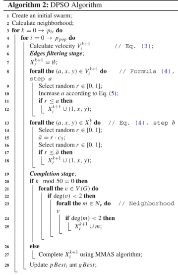
Algorithm 2 shows how the DPSO algorithm uses for-mulas (3) and (4). The first steps involve creating a random particle swarm, based on which the best position is selected, i.e.,g Best. Then, the next velocity of each particle is calcu-lated in accordance with formula (3) (line 5. Algorithm2). The operation of multiplying a given number by a set is car-ried out as a multiplication of that number by each coefficient

afor elements of that set (edges). The probability of choosing a given edge for a particle to go to the next position depends on coefficientsc1,c2,c3and a random variable, i.e.,r and().

Algorithm 2:DPSO Algorithm

1 Create an initial swarm; 2 Calculate neighborhood;

3 fork=0→pi tdo

4 fori=0→ppopdo

5 Calculate velocityV_ik+1 // Eq. (3);

6 Edges filtering stage;

7 Xk_i+1= ∅;

8 forall the(a,x,y)∈V_ik+1do // Formula (4), step a

9 Select randomr∈ [0,1]; 10 Increaseaaccording to Eq. (5);

11 ifr≤athen

12 Xk_i+1∪(1,x,y);

13 forall the(a,x,y)∈Xk_i do // Eq. (4), step b

14 Select randomr∈ [0,1]; 15 a¯=r·c3; 16 Select randomr∈ [0,1]; 17 ifr≤ ¯athen 18 Xk_i+1∪(1,x,y); 19 Completion stage; 20 ifk mod 50=0then 21 forall thev∈V(G)do 22 ifdeg(v) <2then

23 forall them∈N_vdo // Neighborhood v

24 ifdeg(m) <2then

25 X_ik+1∪m;

26 else

27 CompleteXk_i+1using MMAS algorithm; 28 Updatep Bestiantg Best;

This process is responsible for a random selection of edges. In this way, a particle’s next velocity is computed, based on which its next position is established. A new solution is cre-ated in two stages, i.e., filtering and completion. At the first stage, each edge belonging to the set of velocities is copied to a particle’s next position if the value of coefficienta for that edge is higher than the value of random variabler(rows 11. and 17.).

The filtering stage is followed by the completion stage, which is aimed at adding the missing edges so as to cre-ate a complete Hamiltonian cycle. The algorithm that was proposed by Zhong et al. (1997) uses the nearest neigh-bor heuristic for this purpose. The solution that is proposed in this paper employs two techniques: the nearest neighbor heuristic that is based on the α-measure (Helsgaun 2000) and the transition function, which has already been used in ant colony algorithms (Stützle and Hoos 2000). The lat-ter makes use of this feature: Each vertex in a Hamiltonian cycle is a vertex with degree two. After the filtering stage, a list of missing vertices and their degrees is made. Then, by manipulating this list, the algorithm connects vertices by

using the transition function. This modification intensifies the exploration of the search space, which translates the qual-ity of solutions into the amount of pheromone and therefore increases the proposed algorithm’s adaptability. Both meth-ods of completing the set of edges are used according to the principle: For every 50 completion operations that have been conducted by using the transition function, one iteration of the nearest neighbor heuristic is carried out. After creating a complete Hamiltonian cycle, all values representing the probability of selecting edgeaare reset to an initial value of one.

The dominant operation in the DPSO algorithm is the intersection of a pair of solutions, e.g., the current position of a particle andg Best(Eq.3). The time complexity of this operation is critical for the performance of the DPSO algo-rithm. We adopted the following encoding. The Hamiltonian cycle is stored in an array of natural numbers in which the value at indexidenotes the end node of the edge starting at nodei. This encoding allows to calculate the intersection of a pair of Hamiltonian cycles inO(n)time, wherendenotes the size of the problem (the number of nodes). The set of velocities and partial solutions is stored as lists of 3-tuples (a,x,y), wherea ∈ [0,1]denotes the probability of select-ing the edge(x,y),x,y∈V,∀x,yx=y.

5 Results

This section consists of two parts. The first part describes the process of creating a library DTSP instances (tests). The second part presents the results of the experiments conducted. Each calculation was repeated 30 times.

5.1 Parameters of the algorithms

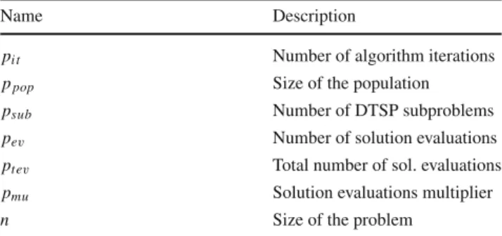
In order to objectively compare the algorithms, a constant fixed number of generated (and evaluated) solutions was adapted as thestopping criterion. On this basis, the values of the remaining parameters of the algorithms were determined, for example, the population size and the number of iterations of an algorithm. Table1contains list of the parameters of the investigated algorithms.

The number of solution evaluations, pev, for each DTSP

instance equals:

pev=pmu·n·pi t·pps

where pi t andpps are the number of iterations of the

algo-rithm and the swarm size, respectively, and pmuis a preset

multiplier. The computations were carried out for a few increasing values ofpmuand, hence, for a few different

num-bers of allowed solution evaluations. The total number of executed iterations (pt ev) was 11·pev because each of the

Table 1 Parameters of the algorithms

Name Description

pi t Number of algorithm iterations

ppop Size of the population

psub Number of DTSP subproblems

pev Number of solution evaluations

ptev Total number of sol. evaluations

pmu Solution evaluations multiplier

n Size of the problem

DTSP instances consisted of 11 subproblems (psub, constant

number in article). The specific values of these parameters that were used in the experiments are shown in Table2.

The parameter values of the MMAS and PACO algorithms were chosen based on suggestions in the literatureStützle and Hoos(2000);Oliveira et al.(2011) and preliminary computa-tions. The parameter values for the MMAS were as follows: number of ants—m = n, wheren is the size of the prob-lem, β = 3,q0 = 0.0, size of the candidate setcl = 30

andρ=0.9—pheromone update coefficient. For the PACO, a fixed number of ants, i.e., ppop = 10, was adapted, as a

result of which the number of iterations for each subprob-lem of the DTSP equaled0.1·pev. This is consistent with

the observations that were presented inCáceres et al.(2014), in which the ACO algorithms were tested for a small com-putational budget. The values of the other parameters for the PACO were: β = 3, q0 = 0.8, cl = 30, α = 0.1

andψ=0.1—pheromone evaporation coefficients for local and global pheromone trail updates, respectively. Also the age-based strategy for updating the pheromone trail from an archive of solutions of size 5 was used.

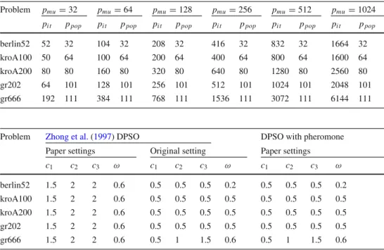
As for the DPSO algorithms, the following parameters were determined (based on Table2): the number of iterations (pi t) and the population size (ppop), which are presented in

Table3. Table4 shows the values of the remaining DPSO parameters.

5.2 DPSO with and without pheromone

During the first phase of the experiments, the DPSO algo-rithms with and without pheromone memory were compared using the static TSP. The aim was to evaluate how the pheromone memory affects the performance of the DPSO. If the implementation of the DPSO algorithm with pheromone allows one to obtain better results than the version without pheromone in the case of the TSP, then this implementa-tion may also allow one to achieve better results for the DTSP. This idea can be justified by the fact that the DTSP can be seen as a sequence of static TSP instances and the information gathered about one instance in the pheromone

Table 2 Number of solution evaluations for a single DTSP subproblem for the DPSO algorithm Problem Evaluations (pev) Name n pmu=32 pmu=64 pmu =128 pmu=256 pmu=512 pmu =1024 berlin52 52 1664 3328 6656 13,312 26,624 53,248 kroA100 100 3200 6400 12,800 25,600 51,200 10,2400 kroA200 200 6400 12,800 25,600 51,200 102,400 204,800 gr202 202 6464 12,928 25,856 51,712 103,424 206,848 gr666 666 21,312 42,624 85,248 170,496 1,875,456 681,984

The values were calculated according to the formula:pmu·n Table 3 Parameters of the

DPSO algorithm for all problem instances

Problem pmu=32 pmu=64 pmu=128 pmu=256 pmu=512 pmu=1024

pi t ppop pi t ppop pi t ppop pi t ppop pi t ppop pi t ppop

berlin52 52 32 104 32 208 32 416 32 832 32 1664 32

kroA100 50 64 100 64 200 64 400 64 800 64 1600 64

kroA200 80 80 160 80 320 80 640 80 1280 80 2560 80

gr202 64 101 128 101 256 101 512 101 1024 101 2048 101

gr666 192 111 384 111 768 111 1536 111 3072 111 6144 111

Table 4 Parameters of the DPSO algorithm with and without pheromone

Problem Zhong et al.(1997) DPSO DPSO with pheromone Paper settings Original setting Paper settings

c1 c2 c3 ω c1 c2 c3 ω c1 c2 c3 ω berlin52 1.5 2 2 0.6 0.5 0.5 0.5 0.2 0.5 0.5 0.5 0.2 kroA100 1.5 2 2 0.6 0.5 0.5 0.5 0.5 0.5 0.5 0.5 0.5 kroA200 1.5 2 2 0.6 0.5 0.5 0.5 0.5 0.5 0.5 0.5 0.5 gr202 1.5 2 2 0.6 0.5 0.5 0.5 0.5 0.5 0.5 0.5 0.5 gr666 1.5 2 2 0.6 0.5 1 1.5 0.6 0.5 1 1.5 0.6

memory may be useful in the context of a modified (next) instance.

Figure4presents the convergence of the two versions of the DPSO algorithm (with and without pheromone) to the optimum for five selected instances of the TSP. In the con-text of a given instance, calculations were repeated with an increasing number of iterations (in accordance with Table3); they were repeated 30 times.

The sets of parameter values are marked with Roman numerals. The numeral “I” denotes values that were adapted for the calculations carried out for the purpose of this paper. These values were determined based on the results of pre-liminary experiments. The values of the parameters of the DPSO (marked as II) that were proposed inZhong et al. (1997) are also presented here for comparison. In the ver-sion without pheromone, the settings that were proposed inZhong et al. (1997) (Zhg(II)) allow one to obtain bet-ter results than the settings for the version with pheromone (Zhg(I)). This is because the algorithm with pheromone complements the probability of choosing a given edge with pheromone reinforcement. The values of scaling

parame-tersc1,c2, c3,ωshould be lower, unlike in the algorithm

version without pheromone, where this reinforcement does not occur. Nonetheless, this comparison was necessary as these settings were contrasted with those that were used in the version with pheromone. The two versions of this algo-rithm have different convergence characteristics. The version with pheromone returns better results for a larger number of iterations, which is due to the pheromone matrix’s demand for learning. This is disadvantageous when the size of the search space and the number of iterations are small. As for thegr666problem, i.e., when the search space is larger, the algorithm without pheromone allowed one to obtain better results only for the smallest number of iterations (192). In any other case, the algorithm version with pheromone pro-duced better results. It was this algorithm that found the best solution for each problem (without taking the number of iter-ations into account). The influence of the growing number of iterations on the quality of the obtained solutions (the distance from the optimum) is also important. This is par-ticularly visible for larger search spaces (from thekroA100

(a)

(b)

(c)

(d)

(e)

Fig. 4 Convergence of the DPSO algorithms to the optimum relative to the number of iterations. “Pher” and “Zhg” denote the implementation of the algorithm with and without pheromone, respectively. Roman numerals (I and II) refer to the values in Table4

with pheromone, there is a large improvement (the line of convergence is almost vertical). The improvement is not vis-ible for the implementation of the DPSO algorithm without pheromone.

5.3 Comparison of the variants of the DPSO

The next series of experiments entailed a comparison of two variants of the DPSO algorithm with pheromone in terms of convergence: one that involves resetting the pheromone matrix (DPSOR+) after each change of the input data and the other one that does not involve resetting the matrix (DPSOR−), in the context of thekroA200instance from the DTSP repository for two different values of changes in the coordinates of vertices (3 and 50%). In the former case, the DPSOR+ algorithm produced results that were 1.95% bet-ter (Fig.5) than those obtained by the version that involves resetting the pheromone matrix (kroA200, 3% of changes in each subproblem). In the latter case (Fig.5), the difference was−0.23%, in favor of the variant that involves resetting the pheromone value after each change of the input data (kroA200, 50% of changes in each subproblem). In the last iteration of the algorithm (before the change of the data), the best solution is marked and information is provided on the variant of the algorithm’s implementation that produced that solution. The two charts show different characteristics of convergence to the optimum, except for the first subproblem, for which the pheromone matrix in both these algorithms was initialized with the same (initial) values.

It can be seen from Fig.5 that the variant that does not involve resetting the matrix in the first iterations of the

algo-rithm has better convergence and that it found a solution that was not much different from the final result. Since the new optimum differs from the previous one in terms of only 10% of edges, the “knowledge about the problem” that has been gathered in the form of pheromone is mostly up to date and it improves the convergence of the algorithm, especially at the initial stage. In subsequent iterations, the pheromone matrix slowly adapts to the new data. After half of all iterations are executed, the convergence rate increases again. As conver-gence is fast at the beginning, the algorithm has more time to find edges that are elements of the optimal solution. This is why the R−version (which did not involve resetting the pheromone value) achieved better results for 9 out of 11 sub-problems.

As shown in Fig. 6, pheromone did not accumulate on good quality edges due to a large number of changes (50%) (there was a large number of changes in the optimum relative to the previous optimum, i.e., from before the changes took place). Therefore, both variants of the algorithm had to adapt the pheromone for new data, and therefore, they explored the best edges that had been found previously to a lesser extent. This does not have an impact on how many better solutions are found (a total of 8 per 11 subproblems), but it does influence a difference that is expressed in percentage points, which is negative and whose absolute value is small (0.23). Therefore, the profit from copying the pheromone matrix (transferring knowledge about the previous solution) was negative. Given that the value of the mean difference was negative and the absolute value was small, it can be stated that the benefit of retaining previous pheromone values was negligible in this case.

Fig. 5 Convergence of the DPSO algorithms to the optimum for the problemkroA200with 3% of changes. R+ and R−denote the version that involves resetting the pheromone value and the version that does

not, respectively.X-axistick marksdenote the moments at which the location of some of the coordinates of vertices (cities) changes

Fig. 6 Convergence of the DPSO algorithm to the optimum for the problemkroA200with 50% of changes. R+ and R−denote the version that involves resetting the pheromone value and the version that does not, respectively

5.3.1 Influence of the number of iterations on the convergence of algorithms

The quality of the solutions that are generated by heuristic algorithms significantly depends on the number of generated solutions. In order to test the convergence of the analyzed variants of the DPSO algorithm, i.e., those that involve reset-ting pheromone memory and those that do not, a range of calculations were carried out for different numbers of iterations of the algorithm which had been determined in

accordance with Table 3. Figures 7 and 8 present charts showing average quality of the solutions that were obtained for versions of the DPSO algorithm that did and did not involve resetting pheromone memory, respectively. As can be seen, together with an increase in the number of iterations of the algorithm, the quality of solutions that are generated improves significantly, and the largest relative improvement in convergence can be observed for smaller values of the iter-ation multiplier (pmu). If the number of iterations was further

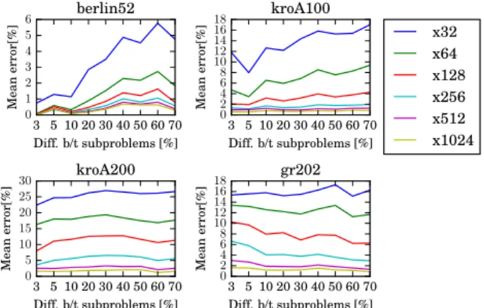
solu-Fig. 7 A comparison of mean relative errors of solutions for the tests berlin52,kroA100,kroA200andgr202in terms of the percentage of the number of vertices that underwent changes for the DPSOR+ algo-rithm (i.e., the DPSO algoalgo-rithm that involves resetting the pheromone value). The consecutive series of data on the charts denote the results for different values of multipliers, in accordance with Table3

Fig. 8 A comparison of mean relative errors of solutions for the tests

berlin52,kroA100,kroA200andgr202in terms of the percentage of the number of vertices that underwent changes for the DPSOR−algorithm (i.e., the DPSO algorithm that does not involve resetting the pheromone value)

tions, but the change would be relatively small, which one can observe by comparing the results for the values of the multiplier: 512 and 1024.

The dominance of the DPSOR− algorithm, in which pheromone memory is not reset after changes that are made to the current subproblem, is also evident. This is particularly visible for the smallest problems, i.e.,berlin52andkroA100.

5.4 Comparison of all algorithms

In order to compare the DPSO algorithms with the MMAS and the PACO, a range of computational experiments was conducted for a set of four instances: berlin52, kroA100,

kroA200andgr202. To check the “extent of usefulness” of pheromone memory for the search process, the behavior of algorithms was tested for the instances of the problem with

an increasing percentage (3, 5, 10, 20, 30, 40, 50, 60 and 70%) of the total number of vertices (cities) whose coor-dinates underwent random changes. Intuitively, when only a small proportion of vertices change their location, the existing knowledge about the search space that is stored in pheromone trails largely remains up to date and makes it easier to find high-quality solutions for a new subproblem. If, however, the extent of changes is very large, for example 60%, one can expect that “old” knowledge about the problem will mostly be outdated.

Figure9presents a box plot of the mean solution error for the DPSO algorithms that involve resetting the pheromone matrix (DPSOR+) and the DPSO algorithms that do not involve resetting the pheromone matrix as well as for the MMAS and PACO algorithms for the problem berlin52. As can be seen, the DPSO algorithm outperforms the other algorithms, especially when the number of vertices whose coordinates undergo modifications between consecutive sub-problems is small. The version of the DPSO algorithm that does not involve resetting the pheromone matrix turned out to be much better than the DPSO algorithm version that does

Fig. 9 Box plot of the relative solution error for theberlin52DTSP instance for the analyzed algorithms. Theboxesare grouped according to the percent of the total number of vertices (cities) whose locations underwent a change

Fig. 10 Box plot of the relative solution error for thekroA200DTSP instance for the analyzed algorithms. Theboxesare grouped according to the percent of the total number of vertices (cities) whose locations underwent a change

Ta b le 5 Results o f statistical comparison of the algorithms considered based o n the mean quality of the solutions obtained Dif f. b etween subproblems [%] 3% 5% 10% 20% 30% 40% 50% 60% 70% T o tal A lg o ri th m (a lg . in d ex ) 123 4 12341234123412341234123412341234 T est berlin52 DPSOR+LS − (1 ) - ---X ---X --X X --X X --X X --X X --X X --X X 1 4 DPSOR − LS − (2 ) X - XX -X X- X XX -X XX-X XX-X X -X XX-X X2 3 M M A S (3 ) X --X -X ---X ---X ---X ---X ---X ---X ---X 1 0 P A C O (4 ) - ---0 T est kroA100 DPSOR+LS − (1 ) - ---X --X X ---X ---X ---X ---X 7 DPSOR − LS − (2 ) X --X X --X X --X ---X --X X ---X ---X ---X ---X 1 3 M M A S (3 ) X X -X X X -X X --X ---X ---X X X -X ---X ---X 1 5 P A C O (4 ) - ---X ---1 T est kroA200 DPSOR+LS − (1 ) - ---0 DPSOR − LS − (2 ) X ---X ---X ---3 M M A S (3 ) XX - XX-X XX - XX - XX -X X- XXX-X XX-X 2 3 P A C O (4 ) X X -X X -X X -X X - XX -X X -X X -X X -X X -1 8 T est gr202 DPSOR+LS − (1 ) - ---X ---X ---X ---X X --X X 7 DPSOR − LS − (2 ) - ---X ---X -X ---X ---X ---X ---X X --X X 1 0 M M A S (3 ) X X -X X ---X X --X ---7 P A C O (4 ) X X -X XX- XXX-X XX -X - X - X-2 0 Nonparametric Mann-Whitne y U test w as used with confidence le v el of 0.05. ’X’ m ark in a cell m eans that the algorithm whose n ame is in the corresponding ro w obtained significantly b etter results than the algorithm w hose inde x is in the corresponding column; ’-’ mark means that there were no statistically significant d if ference b etween the results

involve resetting the pheromone value when the percentage of the number of vertices that underwent changes was not higher than 20%.

A comparison of the algorithms for thegr202instance, which is presented in Fig.10, is more interesting. ACO algo-rithms achieved better results when the problem underwent small changes, i.e., changes that did not amount to more than 5%, whereas the DPSO algorithm proved to be bet-ter when the changes were significant (60 and 70%). This is because the adapted parameter values of the MMAS and PACO algorithms resulted in putting a large emphasis on the exploitation of the search space around the best solutions that had been obtained at the expense of more extensive explo-ration.

All the algorithms were compared in terms of the qual-ity of the results that were produced based on a two-sided, nonparametric Mann–Whitney–Wilcoxon test, with a signif-icance level of 5%. The results of the calculations for the number of evaluationspev=256·11·nare summarized in

Table5. These results vary significantly for some instances. The MMAS algorithm performed significantly better more often than the other algorithms for thekroA100andkroA200

instances. The DPSO algorithm, which did not involve reset-ting the pheromone matrix, obtained good results for the

berlin52 and kroA100 instances. The performance of the PACO was especially good for thegr202instance. When taking into account all four instances, the MMAS obtained significantly better results in 55 cases, the DPSOR− algo-rithm (i.e., the DPSO version of algoalgo-rithm, which did not involve resetting the pheromone value) in 49 cases, the PACO algorithm in 39 cases and the DPSOR+ algorithm in 28 cases. To recapitulate, the ant colony algorithms turned out to be better in a larger number of cases, even though the parameter values of the DPSO were chosen on a per-instance basis, as indicated in Table4. Nevertheless, the performance of the DPSO algorithms, particularly the DPSOR−, is encourag-ing, especially considering the fact that the DTSP can be considereda nativeas problem to the ACO algorithms, i.e., it is discrete and graph based.

6 Conclusions

Dynamic optimization problems have great practical signif-icance. An innovative algorithm for discrete particle swarm optimization (DPSO) is proposed in the present paper; this algorithm has been enriched by pheromone memory which is modeled on ant algorithms. The DPSO searches the solu-tion space because of pheromone that makes use of machine learning and due to the interaction between particles. In this way, it combines the advantages of ant colony algorithms and classical particle swarm optimization. For the purpose of computational experiments, a library of DTSP instances was

developed based on the well-known TSPLIB library (Reinelt 1995). For each test, a dynamic counterpart was prepared which consisted of a series of subproblems that had been created as a result of a random change in the location of a predetermined number of coordinates of cities (vertices). For each subproblem, an optimal solution was determined, which allowed one to clearly evaluate the quality of the results that were obtained for the analyzed algorithms.

The algorithms were tested on four different DTSP instances with 9 different intensities of changes between con-secutive subproblems as well as for 6 different limits on the number of generated solutions (in total, there were 216 com-binations). The quality of the results greatly depended on the computational budget that had been adapted. The aver-age quality of solutions was within 1% from optima for the larger numbers of solutions created. The quality of solutions could have been significantly improved if local search had been applied.

It is worth noting that the use of pheromone memory improves the convergence of the DPSO algorithm for the DTSP. If the differences (coordinates of points) between con-secutive subproblems of the DTSP are relatively small, then the knowledge about the previous subproblem that is accu-mulated in pheromone memory makes it easier to find good solutions for a new subproblem. This is particularly visi-ble when the computational budget that has been adapted is small, which confirms that this algorithm is useful when the problem undergoes frequent changes and the time peri-ods between consecutive changes does not make it possible to carry out long calculations. On the other hand, if the problem rarely undergoes modifications, similar quality results can be obtained by using the DPSO algorithm, in which pheromone memory is reset following each modification of the problem and the algorithm execution is equivalent to separate execu-tions of this algorithm for each of the DTSP’s subproblems. Although the MMAS and PACO algorithms produced bet-ter results in a larger number of cases, this advantage is not big, which shows that the DPSO algorithm is compet-itive. Further studies should take into account local search heuristics and focus on solving larger DTSP instances (with thousands of cities). It will also be interesting to use the DPSO algorithm for other dynamic combinatorial optimiza-tion problems, such as the dynamic vehicle routing problem.

Acknowledgements This research was supported in part by PL-Grid Infrastructure.

Compliance with ethical standards

Conflict of interest The authors declare that they have no potential conflict of interest.

Open Access This article is distributed under the terms of the Creative Commons Attribution 4.0 International License (http://creativecomm ons.org/licenses/by/4.0/), which permits unrestricted use, distribution,

and reproduction in any medium, provided you give appropriate credit to the original author(s) and the source, provide a link to the Creative Commons license, and indicate if changes were made.

References

Applegate D, Bixby R, Chvatal V, Cook W (2006) Concorde TSP solver. http://www.math.uwaterloo.ca/tsp/concorde.html. Accessed 24 Jul 2017

Bilu Y, Linial N (2012) Are stable instances easy? Comb Probab Comput 21(5):643–660

Blackwell T, Branke J, Li X (2008) Particle swarms for dynamic optimization problems. In: Blum C, Merkle D (eds) Swarm Intelli-gence. Natural computing series. Springer, Berlin, Heidelberg, pp 193–217

Boryczka U, Stra˛k Ł (2012) A hybrid discrete particle swarm optimiza-tion with pheromone for dynamic traveling salesman problem. In: Computational collective intelligence. Technologies and applica-tions, lecture notes in computer science, vol 7654. Springer, Berlin, Heidelberg, pp 503–512

Boryczka U, Stra˛k Ł (2013) Efficient DPSO neighbourhood for dynamic traveling salesman problem. In: Computational collective intelligence. Proceedings on Technologies and applications—5th international conference, ICCCI 2013, Craiova, Romania, Septem-ber 11–13, pp 721–730

Boryczka U, Stra˛k Ł (2015a) Diversification and entropy improvement on the dpso algorithm for dtsp. In: Intelligent information and database systems, lecture notes in computer science, vol 9011. Springer International Publishing, Berlin, pp 337–347

Boryczka U, Stra˛k Ł (2015b) Heterogeneous dpso algorithm for dtsp. In: Computational collective intelligence, lecture notes in computer science, vol 9330. Springer International Publishing, pp 119–128 Cáceres LP, López-Ibánez M, Stützle T (2014) Ant colony optimization on a budget of 1000. In: Swarm intelligence, Springer, pp 50–61 Demirta¸s YE, Özdemir E, Demirta¸s U (2015) A particle swarm

opti-mization for the dynamic vehicle routing problem. In: 2015 6th International conference on modeling, simulation, and applied optimization (ICMSAO). IEEE, pp 1–5

Dorigo M, Stützle T (2010) Ant colony optimization: overview and recent advances. In: Gendreau M, Potvin JY (eds) Handbook of metaheuristics. Springer, pp 227–263

Eyckelhof CJ, Snoek M, Vof M (2002) Ant systems for a dynamic tsp: ants caught in a traffic jam. In: Ant algorithms: third international workshop, ANTS 2002, vol 2463/2002 of lecture notes in computer science. Springer, pp 88–99

Goldbarg E, de Souza G, Goldbarg M (2008) Particle swarm optimiza-tion algorithm for the traveling salesman problem. INTECH Open Access Publisher, Rijeka

Guntsch M, Middendorf M (2001) Pheromone modification strategies for ant algorithms applied to dynamic tsp. In: Boers EJW (ed) Applications of evolutionary computing. Springer, pp 213–222 Guntsch M, Middendorf M (2002) Applying population based aco to

dynamic optimization problems. In: Ant Algorithms, Springer, pp 111–122

Guntsch M, Middendorf M, Schmeck H (2001) An ant colony optimiza-tion approach to dynamic tsp. In: Proceedings of the 3rd annual conference on genetic and evolutionary computation. Morgan Kaufmann Publishers Inc., San Francisco, CA, USA, GECCO’01, pp 860–867.http://dl.acm.org/citation.cfm?id=2955239.2955396 Helsgaun K (2000) An effective implementation of the Lin–Kernighan

traveling salesman heuristic. Eur J Oper Res 126:106–130 Hu X, Shi Y, Russell E (2004) Recent advances in particle swarm. In:

Congress on evolutionary computation, CEC2004, vol 1, pp 90–97

Kalivarapu V, Foo JL, Winer E (2009) Improving solution character-istics of particle swarm optimization using digital pheromones. Struct Multidiscip Optim 37(4):415–427

Kang L, Zhou A, McKay RI, Li Y, Kang Z (2004) Benchmarking algo-rithms for dynamic travelling salesman problems. In: Proceedings of the IEEE congress on evolutionary computation, CEC 2004, 19–23 June 2004, Portland, OR, USA, pp 1286–1292

Kennedy J, Eberhart R (1995) Particle swarm optimization. In: Proceed-ings of the IEEE international conference on neural networks, pp 1942–1948

Khouadjia MR, Jourdan L, Talbi EG (2010) Adaptive particle swarm for solving the dynamic vehicle routing problem. In: 2010 IEEE/ACS international conference on computer systems and applications (AICCSA). IEEE, pp 1–8

Li W (2011) A parallel multi-start search algorithm for dynamic trav-eling salesman problem. In: Proceedings of the 10th international conference on experimental algorithms

Li C, Yang M, Kang L (2006) A new approach to solving dynamic trav-eling salesman problems. In: Proceedings of the 6th international conference on simulated evolution and learning. Springer, Berlin, Heidelberg, SEAL’06, pp 236–243

Mavrovouniotis M, Yang S (2010) Ant colony optimization with immi-grants schemes in dynamic environments. In: Schaefer R, Cotta C, Kołodziej J, Rudolph G (eds) Parallel problem solving from nature, PPSN XI, lecture notes in computer science, vol 6239. Springer, Berlin, Heidelberg, pp 371–380

Mavrovouniotis M, Yang S, Yao X (2012) A benchmark generator for dynamic permutation-encoded problems. Springer, Berlin Mavrovouniotis M, Li C, Yang S (2017) A survey of swarm intelligence

for dynamic optimization: algorithms and applications. Swarm Evolut Comput 33:1–17

Mori N, Kita H (2000) Genetic algorithms for adaptation to dynamic environments—a survey. In: Industrial electronics society, 2000. IECON 2000, 26th annual conference of the IEEE, vol 4, pp 2947– 2952

Okulewicz M, Ma´ndziuk J (2013) Application of particle swarm optimization algorithm to dynamic vehicle routing problem. In: International conference on artificial intelligence and soft com-puting. Springer, pp 547–558

Oliveira SM, Hussin MS, Stützle T, Roli A, Dorigo M (2011) A detailed analysis of the population-based ant colony optimization algorithm for the tsp and the qap. In: Proceedings of the 13th annual confer-ence companion on Genetic and evolutionary computation. ACM, pp 13–14

Pedemonte M, Nesmachnow S, Cancela H (2011) A survey on paral-lel ant colony optimization. Appl Soft Comput 11(8):5181–5197. doi:10.1016/j.asoc.2011.05.042

Pintea CM, Pop PC, Dumitrescu D (2007) An ant-based technique for the dynamic generalized traveling salesman problem. In: Pro-ceedings of the 7-th WSEAS international conference on systems theory and scientific computation, pp 257–261

Pintea C, Crisan GC, Manea M (2012) Parallel ACO with a ring neighborhood for dynamic TSP. JITR 5(4):1–13. doi:10.4018/jitr. 2012100101

Pop PC, Pintea C, Dumitrescu D (2009) An ant colony algorithm for solving the dynamic generalized vehicle routing problem. Civil Eng 1(11):373–382

Psaraftis H (1988) Dynamic vehicle routing problems. Veh Routing Methods Stud 16:223–248

Reinelt G (1995) TSPLIB95. Interdisziplinäres Zentrum für Wis-senschaftliches Rechnen (IWR). Heidelberg

Stützle T, Hoos HH (2000) Max-min ant system. Future Gener Comput Syst 16(8):889–914

Tinós R, Whitley D, Howe A (2014) Use of explicit memory in the dynamic traveling salesman problem. In: Proceedings of the 2014 annual conference on genetic and evolutionary computation.

ACM, New York, NY, USA, GECCO ’14, pp 999–1006. doi:10. 1145/2576768.2598247

Yang S, Yao X (2013) Evolutionary computation for dynamic optimiza-tion problems. Springer, Berlin

Younes A, Basir O, Calamai P (2003) A benchmark generator for dynamic optimization. In: Digest of the Proceedings of the wseas conferences

Younes A, Calamai P, Basir O (2005) Generalized benchmark gen-eration for dynamic combinatorial problems. In: Proceedings of the 7th annual workshop on genetic and evolutionary computation ACM, New York, NY, USA, GECCO ’05, pp 25–31. doi:10.1145/ 1102256.1102262

Zhong Wl, Zhang J, Chen Wn (1997) A novel set-based particle swarm optimization method for discrete optimization problems. In: Evolutionary computation, 2007. CEC 2007, vol 14. IEEE, pp 3283–3287