Durham Research Online
Deposited in DRO:
05 November 2015
Version of attached le:
Accepted Version
Peer-review status of attached le:
Peer-reviewed
Citation for published item:
Akperi, B.T. and Matthews, P.C. (2014) 'Analysis of clustering techniques on load proles for electrical distribution.', in POWERCON 2014 Chengdu : 2014 International Conference on Power System Technology : Towards green, ecient and smart power system. Proceedings of a meeting held 20-22 October 2014,
Chengdu, China. , pp. 1142-1149.
Further information on publisher's website:
http://dx.doi.org/10.1109/POWERCON.2014.6993986Publisher's copyright statement:
c
2014 IEEE. Personal use of this material is permitted. Permission from IEEE must be obtained for all other uses, in any current or future media, including reprinting/republishing this material for advertising or promotional purposes, creating new collective works, for resale or redistribution to servers or lists, or reuse of any copyrighted component of this work in other works.
Additional information:
Use policy
The full-text may be used and/or reproduced, and given to third parties in any format or medium, without prior permission or charge, for personal research or study, educational, or not-for-prot purposes provided that:
• a full bibliographic reference is made to the original source
• alinkis made to the metadata record in DRO
• the full-text is not changed in any way
The full-text must not be sold in any format or medium without the formal permission of the copyright holders.
Please consult thefull DRO policyfor further details.
Durham University Library, Stockton Road, Durham DH1 3LY, United Kingdom Tel : +44 (0)191 334 3042 | Fax : +44 (0)191 334 2971
Analysis of Clustering Techniques on Load Profiles
for Electrical Distribution
Brian Akperi
School of Engineering and Computing Sciences
Durham University Durham, United Kingdom Email: [email protected]
Peter Matthews
School of Engineering and Computing Sciences
Durham University Durham, United Kingdom Email: [email protected]
Abstract—The classification of electrical load profiles has become increasingly important as a driver for distribution companies in understanding substation data. The daily load profile can often give great insight into the types of customers connected to the substation and can assist with developing a long-term forecast. The literature in this area often uses data mining and clustering techniques to determine a load diagram representative for a subset of customers or substations. The type of technique used can often lead to representative load diagrams of unique shapes with differing numbers of customers belonging to each group.
This paper analyses clustering techniques on representative load diagrams for primary substations at the distribution level. In particular, this paper will analyse clustering techniques in terms of their performance and effect on load profile groupings. The results show that K-means clustering showed the best performance in generating unique, well-populated cluster groups. This gives a greater understanding of the divisions between substations which can be used for future forecasting.
Index Terms—Clustering methods, Power distribution, Load modeling
I. INTRODUCTION
It is necessary for distribution network operators to gain more insight into annual demand trends in order to plan for future scenarios. This includes the fact that electric demand is expected to increase but there is an additional expected impact from new technologies such as electric vehicles and heat pumps. For this research, the demand data is collected using SCADA (supervisory control and data acquisition) systems from primary substations at 30 minute intervals giving a daily load profile with 48 points. The primary figure needed from this is the maximum demand for each substation on an annual basis which all future forecasts are based on. This will give justification for any necessary reinforcement needed on the network before firm capacity is exceeded.
The motivation for examining daily load profiles in particular comes from the need to determine underlying trends within the annual load profile. Because of industry knowledge, it is accepted that there are seasonal and day of the week variations in load profiles. Therefore by examining
the different periods separately, it is possible to see seasonal demand variation. An additional motivator is analysing the flattening of demand profiles. In this case, it is defined as the difference between the summer trough and winter peak demand. Any difference in daily load profile will help to explain this difference. It is also good to reaffirm the types of customer belonging to any daily load profile. The shape of a load profile is often indicative of the mixture of domestic and commercial/industrial customers and will aid engineering judgment. The final motivator comes from a need to separate primary substations on the distribution network into groups to aid the forecasting process. Substations with similar load profiles are more likely to have similar long-term profiles. Therefore any forecasting algorithms can act on these groups separately and potentially reduce error and increase reliability.
One method of analysis that has proven to be popular in another literature survey [1] is to determine representative daily load profiles for a substation by data mining methods. These load profiles can then be used to categorise substations based on their daily load for improved forecasts. In particular, various clustering techniques can be used to build these load profiles. However, each method can lead to load profiles of different shape with differing numbers of customers belonging to each cluster.
This paper will look at three popular clustering methods and their effect on load profile data. This will be done by a discussion of each individual method along with the use of clustering validity metrics. Section II explores some of the related work in the area. Section III gives an overview of the methods used in the paper. Section IV details the methodology used for the clustering process. Section V applies the methodology and discusses the obtained results. Section VI justifies the connection of this work to a future forecasting algorithm. Section VII summarises the results by discussing which algorithm performed the best and what impact this will have on future forecasting.
II. RELATEDWORK
In the literature, load profile clustering has been investigated [1] [2] [3], but there are gaps where there is room for new research. In particular, [1] also looks at various clustering techniques for load profile classification but pre-partitions the data by type of customer. However, in this work the customer data is used to support the load profiles obtained and assumes no prior knowledge. Additionally, the distribution level is considered at primary substations operating at 11/33/66 kV levels. These substations consist of several different types of customers including domestic, commercial and industrial so individual customers cannot be considered. Any consideration of customer mixture would have to be realised post clustering. Also in [1], much of the focus is on the use of different clustering validity metrics to judge how well each clustering technique works with little to no discussion on the effect of the methods themselves on the specific data set used.
An investigation into load profile clustering was also carried out by Western Power Distribution in their Low Voltage (LV) network templates project [4]. Using clustering and their own customer database, they developed daily load profiles for distinct customer mixtures on their network. However, it lacked a detailed explanation of clustering methods and opted on a single one (hierarchical) leaving room for fur-ther research. This study will be unique in the analysis of multiple clustering techniques on distribution level substation data while considering not only the typical clustering validity metrics but also the methodology of each individual clustering technique.
III. THEORY ANDMETHODSUSED
In order to create groups to improve upon both engineering understanding and to improve future forecasting, a few classic clustering algorithms will be used. These particular methods were chosen because of their use in similar studies [1] [4] and because of their familiarity [5]. In subsections A, B and C, an overview of the clustering methods used will be given. In subsection D, an overview of the metrics used will be given. Finally, in subsection E, a link to an engineering context is given by association with the customer types on the network. A. K-Means Clustering
K-means clustering [6] is one of the most popular clustering techniques used across various disciplines on a wide variety of data. The basic steps of the algorithm are as follows:
1) Choose number of K clusters.
2) Assign data points to a cluster centre based on a distance metric.
3) Calculate the mean of each cluster group which becomes the new centre.
4) Repeat 2-3 until all data points are assigned to the same cluster.
Although this is a simple method that is widely used, there are classical problems associated with this method. One of the disadvantages is that the initial random choice of cluster
centres can often cause very different clusters to form. A popular technique to address this as suggested in [5] and [7] is to run the algorithm several times and choose the solution with the lowest sum of squared distance between the data and cluster centroids. Furthermore, there is also the issue of sensitivity to outliers as all points are forced into clusters. This will be considered when analysing the shapes of each cluster. Finally there is always the issue of the choice of number of
K clusters as addressed in subsection III-D. B. Hierarchical Clustering
The hierarchical clustering method is based on a tree struc-ture known as the dendrogram [5]. This can be done in a top down approach known as the divisive method which starts at a single cluster and performs binary splits until all clusters only have one member. However, this method is computationally intensive and not often used. More commonly used is the agglomerative method which is a bottom up approach built starting from single member clusters and combining clusters until there is only one cluster. The algorithm is as follows:
1) Start with N clusters where N is the number of data points.
2) Combine clusters based on a linkage method starting from the clusters which are closest together.
3) Add the newly formed cluster to the distance matrix. 4) Repeat 2-3 until there is only one cluster containing all
elements.
The choice of linkage method for hierarchical clustering will also have to be considered. In [8] some of the most common linkage methods are summarised. The average linkage method is seen as being one of the most robust methods and is the average distance between all pairs of data points where one comes from each group. This is in contrast to simpler methods known as single linkage (nearest neighbour) and complete linkage (furthest neighbour) where distance is simply calculated by the nearest or furthest points in each group. An additional linkage criteria known as Ward’s method was also considered by [1] but it was found that average linkage was better at rejecting dissimilar load profiles whilst Ward attempted to find groups of the same size. A choice of number of clusters must be made here by choosing a threshold horizontal division on the dendrogram.
C. Fuzzy C-means Clustering
In this type of clustering, data points do not have to belong to a single cluster but instead have degrees of membership in[0,1]that denote the extent to which a point is similar to that cluster centre. Otherwise, the procedure is quite similar to K-means with the following steps:
1) Choose number ofKclusters and initialise random centre points.
2) Update the membership matrix U by uij = PK v=1 d(xi,cj) d(xi,cv) m1−1 −1 , where uij ∈ U is the fuzzy membership matrix, d(·,·) is a chosen distance metric such as Euclidean distance,xi∈X is the matrix
of load profiles, cj is the cluster centre and m > 1 is the fuzzification parameter.
3) The matrix of cluster centres C = (ci) is then updated
ci= PN j=1(uij)mxj PN j=1(uij)m ,i= 1, ..., K
4) Repeat 2-3 until the matrix of centres stabilises.
The disadvantages of using fuzzy C-means are similar to using K-means in that there is no definitive method to identify the initial partitions and that the method is sensitive to outliers. The uniqueness of fuzzy membership can offer more insight than crisp clustering because it can help to show the uniqueness (or non-uniqueness) of the cluster centres and the similarity of load profiles to the centres.
D. Clustering Validity
In order to attain supporting evidence for the engineering based explanations of the cluster solutions, clustering validity metrics will be used. These metrics can be used to ascertain both the effectiveness of one clustering algorithm versus another and to determine the number of clusters that should be used. For crisp clustering, a couple of popular indices are used here: Dunn’s index and Davies-Bouldin.
Dunn’s index is a popular method in the literature and identifies compact and separate clusters [10]. The Dunn index
T is defined as T = min 1≤i≤c min 1≤j≤c,j6=i min xi∈Xi,xj∈Xj (d(xi, xj)) max 1≤k≤cyk (1)
wherexi∈Xi is a cluster group of vectors,c is the number of clusters used, d(·,·) is the standard Euclidean distance metric, and yk = max
xl,xm∈Xk(xl, xm). The best solution is the one with the highest Dunn’s index.
The Davies-Bouldin (DB) criterion is defined as a ratio of within cluster and between cluster differences [9]. SupposeSi and Sj are dispersion measures which are the average dis-tances between each point in the clusters and their respective centroids.Mij is the Euclidean distance between theith and
jth clusters. Then the DB index R¯ is
¯ R= 1 N N X i=1
maxi6=j{Ri,j}, Ri,j=
Si+Sj
Mi,j
. (2) The best clustering solution is the one with the smallest DB index.
For fuzzy clustering, the allowance for partial membership requires a different clustering validity metric. One of the most popular metrics in use is the Xie-Beni metric [11] which is defined as S= c P i=1 n P j=1 U2 ijkVi−xjk2 nmin i,j kVi−Vjk 2 (3)
where c is the total number of clusters, n is the number of vectors (in this case substations), Uij is an entry in the fuzzy
membership matrix,Viis a cluster centroid, andxjis a vector in the data set. The best solution is one with the lowest Xie-Beni index.
E. Association with Customer Type
Regardless of clustering technique used, it is desirable to have an idea of the types of customer associated to each substation. By using the PCA investigation in [12] it is possible to attribute a customer make-up to each of the primary substa-tions. In particular, there is a need to distinguish between do-mestic customers and commercial/industrial customers. Within domestic customers, there is also a distinction between rural and urban domestic customers. In [12], it was determined that the first principal component (PC1) shows a distinction between domestic and commercial/industrial customers where a positive values indicates a greater influence from commer-cial/industrial customers and a negative value indicates greater influence from domestic customers. The second principal component (PC2) shows a distinction between rural and urban customers where a positive value indicates a greater influence from rural customers and a negative value indicates a greater influence from urban customers. By making this association, it will give supporting evidence for an engineering explanation of resultant clusters. This is useful as both an explanation of the load profiles themselves and as insight into the differences between the clustering techniques.
IV. METHODOLOGY
Initially, each clustering technique will be analysed separately and representative load profiles for the summer period are considered. There are multiple ways a normalisation process can be done. In this paper, the following will be used. Each substation on the network has an annual demand profile consisting of readings taken every 30 minutes. The summer period is defined as June 1 2012-August 31 2012 for a total of 4416 readings. According to the investigation in [4], it is more appropriate to normalise each daily load profile and then average over a period of time as opposed to averaging the period first and then normalising. This helps to highlight daily load patterns and is not as subject to seasonal variation. Normalising by the maximum of each day and then averaging over the summer period is the procedure followed here to attain the representative load profiles.
Before the clustering is done, the number of K clusters needs to be determined for each method. Depending on the criteria used, a different number of chosen clusters could be indicated.
There are three main pieces of information that will inform the discussion for each method. First are the cluster centroids and how the load profile changes over the course of the day. The cluster centroids are generated directly for K-means and fuzzy C-means. For hierarchical clustering, the profiles belonging to each cluster can be averaged to generate a
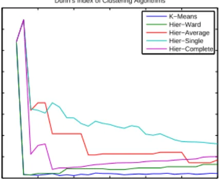
0 5 10 15 20 25 30 0 0.1 0.2 0.3 0.4 0.5 0.6 0.7 0.8 Number of Clusters Dunn’s Index
Dunn’s Index of Clustering Algorithms
K−Means Hier−Ward Hier−Average Hier−Single Hier−Complete
Fig. 1. Dunn’s Index for Crisp Clustering Algorithms
centroid.
Second are the population sizes of the clusters. These are easily gained for K-Means and hierarchical clustering. For fuzzy C-means, because of partial membership, a different method must be used. The membership values across the membership matrix U are summed to attain population sizes. Third are the principal component values from [12] for each cluster centroid. As explained in section III, this allows for an idea of the customer make-up to be understood for each cluster. For K-means and hierarchical clustering, these are the average values of PC1 and PC2 for each cluster. Associating the customer classification principal components from [12] is not as straightforward for fuzzy clustering because of the allowance for partial membership. However, the impact of the PCA can still be discussed with simple matrix multiplication. Let U be a c×m matrix of fuzzy cluster memberships where m is the total number of substations and c is the number of clusters and let V be the
m ×2 matrix which contains the first two PC scores for each substation. Then the matrix W =U V is ac×2 matrix which contains the summation of the PC scores for each cluster weighted by the cluster membership of the substations. After the discussion of each method, the clustering validity metrics will be discussed further in the context of the clusters and any differences between the methods will be highlighted and explained.
V. RESULTS ANDDISCUSSION
A. Choice ofK Number of Clusters
The Dunn index in Fig. 1 shows that K-means and Ward’s linkage criteria performed the worst. However, upon closer inspection it was found that the average, single and complete methods had most of the substations in a single cluster, making this misleading. The size of clusters for K-means and Ward’s linkage are shown in their respective sections. For the choice of K, considering local maximums in a small neighbourhood,K∈[9,14]is appropriate for Ward’s linkage. For K-means, there is no clear local maximum so based
0 5 10 15 20 25 30 0.2 0.4 0.6 0.8 1 1.2 1.4 1.6 1.8 Number of Clusters DB Index
DB Index of Clustering Algorithms
K−Means Hier−Ward Hier−Average Hier−Single Hier−Complete
Fig. 2. DB Index for Crisp Clustering Algorithms
5 10 15 20 25 30 0 0.2 0.4 0.6 0.8 1 Number of Clusters Xie−Beni Index
Xie−Beni Index for Fuzzy C−Means
Fig. 3. Xie-Beni Index for Fuzzy C-Means
on K ∈ [9,14] being a good choice for Ward’s linkage,
K = 9 clusters are chosen. The smallest number of clusters is preferable whenever possible for ease in understanding.
The choice of K according to the DB index in Fig. 2 is less clear. There is a local minimum for Ward’s linkage at
K= 9but there is also one at K= 6. For K-means, there is a local minimum at K = 8 but the differences between for nearby values ofK are small. Since the choice ofK= 9has the most supporting evidence, it is used for subsection V-B and V-C.
For fuzzy clustering, the Xie-Beni index in Fig. 3 shows a general decrease as the number of clusters is increased which would suggest choosing a high number of clusters. As discussed earlier, this can be counterintuitive for the desire to achieve an engineering based explanation of load profile shapes. This problem is acknowledged in [11] and proposes a few ways to address this. One way to do this is by considering the maximum number of clusters n−1
to be where there is a monotonically decreasing value of S afterwards. Then select the lowest value of S in
c ∈ [2, n−1]. However, there may not be a point at which the series is monotonically decreasing. Instead, using prior knowledge thatcna local minimum can be selected. Here, a value of 12 clusters is chosen as it is a clear local maximum.
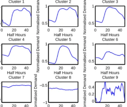
0 20 40 0.5 1 Half Hours Normalised Demand Cluster 1 0 20 40 0.5 1 Half Hours Normalised Demand Cluster 2 0 20 40 0.5 1 Half Hours Normalised Demand Cluster 3 0 20 40 0.5 1 Half Hours Normalised Demand Cluster 4 0 20 40 0.5 1 Half Hours Normalised Demand Cluster 5 0 20 40 0.5 1 Half Hours Normalised Demand Cluster 6 0 20 40 0.5 1 Half Hours Normalised Demand Cluster 7 0 20 40 −1 −0.5 Half Hours Normalised Demand Cluster 8 20 40 0 0.2 0.4 Half Hours Normalised Demand Cluster 9
Fig. 4. Clusters Gained By K-means
TABLE I
K-MEANSCLUSTERINGPOPULATIONS ANDPRINCIPALCOMPONENT
VALUES Population PC1 PC2 Cluster 1 60 0.101 0.155 Cluster 2 162 -0.164 -0.262 Cluster 3 72 2.969 -0.067 Cluster 4 127 0.297 0.224 Cluster 5 53 1.063 1.166 Cluster 6 27 -1.207 -0.474 Cluster 7 63 -2.231 -0.466 Cluster 8 8 N/A N/A Cluster 9 4 1.851 1.665
With regards to clustering validity in general, the choice of a number of clusters is not simply the point at which the chosen metric gives the most favourable value. Instead, the application must be considered and choosing a local minima/maxima in a predetermined neighbourhood usually provides a good compromise between minimising/maximising the metric and an understandable number of clusters.
B. K-Means Clustering
After performing K-means clustering on the summer representative load profiles, Fig. 4 shows the candidate nine cluster centres and their cluster sizes in Table I. By cross referencing with the work in [4] and using general knowledge of load profiles, it is possible to attain a descriptive reference for these clusters. Note that N/A in these tables means there is no available customer data for these clusters because none of the substations have associated customer data. Clusters 1 and 2 follow a typical domestic type load profile which peaks in the early evening around 6 p.m. and has a fairly flat profile throughout the middle of the day. In [4], profiles of this shape are said to have high domestic dominance. In Table I, the PC1 values for clusters 1 and 2 are small and close to 0 showing that there is influence from both domestic and commercial customers.
Clusters 3, 4, and 5 have a much earlier peak around midday with a steady decrease afterwards. In [4], these types of load profiles are said to have a high commercial/industrial
influence. Table I supports this since the PC1 values are more skewed to the positive end indicating a greater influence from commercial/industrial customers.
Cluster 7 is a mostly flat profile which is typically attributed to commercial and industrial customers using the same level of energy throughout the day. However, this is not supported by the PCA as the value for PC1 is negative and indicates a higher influence from domestic customers. This suggests that either the PCA is not accurate enough or that for this particular data set, these flat daily load profiles are attributed to domestic customers even if it is not generally the case.
Clusters 6, 8 and 9 are anomalous load patterns with small populations that do not fit into the other categories. Note that in cluster 8 are substations on the network that are completely generation.
One of the disadvantages of the K-means algorithm is its sensitivity to outliers and noise. As the number of clusters is increased, the probability of an outlier distorting a cluster centroid decreases. Even in this example of nine clusters, there are a couple of clusters (8 and 9) which are sparsely populated and could be classified as outlier clusters. Therefore for K-means, the choice ofK and population of each cluster is important when considering the effect of outliers. If only a few clusters are chosen then it may become a concern for the engineer.
The K-means algorithm mostly performed well here based on the fact that these profile shapes are commonly seen in the industry and that they can be supported by previous works with regards to customer types.
C. Hierarchical Clustering
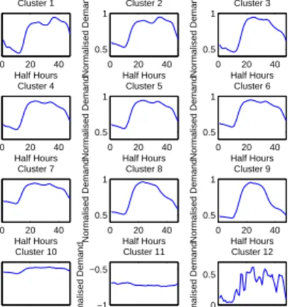
Hierarchical clustering with Ward’s linkage criteria is applied for this example and nine prospective cluster centroids are shown in Fig. 5. These are generated by averaging the profiles of the substations in each cluster after the selection of nine clusters are made. According to [8], Ward’s method will tend to find clusters which are the same size. The cluster populations shown in Table II do not corroborate with this however as some of the clusters are not well populated. Four of the nine clusters contain 95% of the total population.
The load profiles that are well populated do show some of the shapes given by other clustering methods. In particular, clusters 1 and 2 show a load profile with two peaks. This suggests that at least in part that these are clusters that contain the prototypical domestic load profile with a peak around midday, a slight decrease in the afternoon followed by the daily peak in the evening. However, the two peaks are nearly identical which suggests that these profiles were offset in time.
20 40 −0.5 0 0.5 Half Hours Normalised Demand Cluster 9 0 20 40 −0.5 0 Half Hours Normalised Demand Cluster 5 0 20 40 0.5 1 Half Hours Normalised Demand Cluster 8 0 20 40 0.5 1 Half Hours Normalised Demand Cluster 7 0 20 40 0.5 1 Half Hours Normalised Demand Cluster 1 0 20 40 0.5 1 Half Hours Normalised Demand Cluster 2 0 20 40 0.5 1 Half Hours Normalised Demand Cluster 4 0 20 40 −1 −0.5 Half Hours Normalised Demand Cluster 6 0 20 40 0.5 1 Half Hours Normalised Demand Cluster 3
Fig. 5. Clusters Gained By Hierarchical Clustering
TABLE II
HIERARCHICALCLUSTERINGPOPULATIONS ANDPRINCIPAL
COMPONENTVALUES Population PC1 PC2 Cluster 1 172 -0.061 -0.238 Cluster 2 159 1.636 -0.076 Cluster 3 142 -1.268 -0.016 Cluster 4 73 1.047 1.354 Cluster 5 3 N/A N/A Cluster 6 5 N/A N/A Cluster 7 15 -1.066 -0.147 Cluster 8 6 -0.918 1.437 Cluster 9 1 -1.851 1.665
Another issue is that these profiles are extremely similar in shape which is not desirable considering only nine clusters out of a total 576 substations are considered. When checked against the figures from the PCA analysis in Table II, it suggests that cluster 1 contains more load profiles with a domestic influence and cluster 2 contains more profiles with an industrial/commercial influence. This is not made clear in the shapes of the load profiles which makes this method less useful for both future forecasting purposes and in a more general sense for understanding.
The main issue with hierarchical clustering is that once two items are grouped in the dendrogram, they are no longer considered in future iterations of the algorithm. This is of great importance here because distinct and populated clusters are required for understanding. More linkage methods are considered in subsection V-A.
D. Fuzzy C-means Clustering
Fuzzy C-means clustering is unique among these methods in that substations do not have to belong to a single cluster. Instead, they are given membership values in[0,1]that denote the degree to which the daily load profile shape matches the centre point with a value of 0 being the weakest and 1 being the strongest. Similarly to other methods used, the load profile centres in Fig. 6 can be explained using general knowledge of load profiles but also using the preliminary work done in [12]. By performing a summation across the membership matrix
U, Table III shows the number of substations belonging to
0 20 40 0.5 1 Half Hours Normalised Demand Cluster 1 0 20 40 0.5 1 Half Hours Normalised Demand Cluster 2 0 20 40 0.5 1 Half Hours Normalised Demand Cluster 3 0 20 40 0.5 1 Half Hours Normalised Demand Cluster 4 0 20 40 0.5 1 Half Hours Normalised Demand Cluster 5 0 20 40 0.5 1 Half Hours Normalised Demand Cluster 6 0 20 40 0.5 1 Half Hours Normalised Demand Cluster 7 0 20 40 0.5 1 Half Hours Normalised Demand Cluster 8 0 20 40 0.5 1 Half Hours Normalised Demand Cluster 9 0 20 40 0.5 1 Half Hours Normalised Demand Cluster 10 0 20 40 −1 −0.5 Half Hours Normalised Demand Cluster 11 0 20 40 0 0.5 Half Hours Normalised Demand Cluster 12
Fig. 6. Clusters Gained By Fuzzy C-means Clustering
TABLE III
CLUSTERSGAINEDBYFUZZYC-MEANSCLUSTERING
Population PC1 PC2 Cluster 1 48 34.523 -3.274 Cluster 2 68 -8.645 -8.588 Cluster 3 49 58.302 3.469 Cluster 4 65 21.579 -3.109 Cluster 5 72 12.539 -1.201 Cluster 6 75 9.090 -2.847 Cluster 7 63 -28.894 -5.132 Cluster 8 56 41.423 20.608 Cluster 9 35 15.092 22.458 Cluster 10 32 -31.580 -5.398 Cluster 11 7 0.213 0.191 Cluster 12 5 0.580 0.821
each cluster rounded to the nearest whole number.
The first principal component indicates the contribution of commercial/industrial customers where a positive value indicates a greater dominance of commercial/industrial customers while a negative value indicates a greater dominance of domestic customers. The clusters where this value is the highest are in clusters 1, 3, 4, 5, 6, 8 and 9. All except cluster 1 have no distinct second peak and are consistent with industrial load profiles in industry and as shown in [4]. The load profile in cluster 1 is more often associated to more domestic load profiles so this result is surprising. This could be due to the fuzzy clustering algorithm itself since these substations could be outliers in the principal component space which are then exacerbated by the matrix multiplication.
The lowest PC1 values are in clusters 2, 7 and 10 where cluster 2 does exhibit a domestic load profile but 7 and 10 do not. Again, this could be due to the allowance for partial membership as 7 and 10 are much flatter profiles than what is expected of a domestic load profile.
Half-Hourly SCADA Data Averaging & Normalisation Verification & Confidence Bounds Annual Maximum Clustering Monthly Forecasting Group 1 Group n Group 2. . .
Fig. 7. Schematic for Long-term Forecast
of rural (positive values) and urban (negative values) domestic customers. The highest positive values in clusters 8 and 9 show load profiles with the earliest decrease in demand more consistent with industrial load profiles. This follows naturally as one would expect more rural housing in these areas.
Overall, it seems that although fuzzy clustering can be more insightful because of relaxing the hard membership criteria, it is less useful when attempting to gain a general overview of substation behaviour. This is compounded by the fact that PCA already loses information when reducing the high dimensionality of the original space. For the analysis here, fuzzy clustering of load profiles is not seen as appropriate. E. Comparison between Methods
Analysing the crisp clustering techniques first, the main difference that can immediately be seen is in the distribution of the population between clusters. For K-means, the population is well spread out with only two clusters (8 and 9) containing less than 10 substations. As noted earlier for Ward’s linkage, 95% of the substations are grouped in four out of nine clusters. This disparity can be attributed to the way in which the algorithms group data. The methods both use Euclidean distance as a metric for clustering but K-means allows for substations to be reassigned after updating cluster centres. This allows for more distinct cluster groups to be formed. For example, clusters 3 and 4 are given as distinct clusters in K-means but there is no analogous cluster for the K-means cluster 3 in hierarchical clustering.
Fuzzy clustering does offer the potential for more insight but the method offered the least corroboration with the principal component analysis in [12]. The method produced cluster centres of a similar nature to the crisp methods but with inconsistent customer values. For the purposes here, the partial membership proved to be more of a hindrance because it made analysing the total cluster more difficult.
Regarding the clusters in general, it is desirable for each cluster centroid to be unique in shape with the clusters gener-ally having significant numbers in population size. Apart from a good computational performance criteria, there is also a need for human interpretation. If the clusters appear similar visually
or the population is mostly contained in a small number ofn
clusters where n K then the clustering has lost much of its purpose. Arguably, if the initial data set contains many instances in close proximity to each other then this cannot be helped. However, here there is prior knowledge that on a distribution network of this level that there will be unique profiles each with a healthy population size. The load profiles shown in [4] are evidence of this. Based on this reasoning and the best support of the customer data, K-means is seen as the most appropriate method.
VI. LINKS TOFORECASTING
The goal of developing these clustered groups is not only to gain greater insight into the types of daily load profile but also to assist with future forecasting methodology. The literature supports the use of clustering prior to the use of a clustering algorithm. The work in [13] clusters load curves using K-means clustering for forecasting short-term daily peak loads in a heat system. They state that the goal of the clustering is to find characteristic patterns that determine changes in demand peaks. Then a family of functional regression models which helps forecasting can be obtained based on the clusters.
The work in [14] also clusters peak load using self organising maps and then forecasts daily peak loads using a neural network model. Within each cluster, days of the week and holidays are also separated as input data to the neural network. Using standard error metrics such as mean absolute error and mean squared error, it was shown that this hybrid approach is more effective than forecasting on unclustered data.
These papers and other works mostly are forecasting in the short-term one day into the future. The aim of this research is to develop a long-term annual forecast. For example, this would involve using higher level data such as monthly maximum peaks and then selecting the maximum among them. The problem that must be addressed is the use of daily load clusters in a long-term forecast. The key is that each primary substation on the distribution network has a unique annual load profile. If there is a correlation between the daily load profile and annual load profile then improved results
such as in [14] would be expected because there are similar characteristics between the load profiles within each cluster. Further work could be done to establish this correlation more concretely but based on engineering knowledge, this is expected to exist.
The work here and in [4] shows that daily load profile characteristics can mostly be attributed to the customers at that substation. As a generalisation, substations which have demand that is more flat throughout the day with a distinct maximum are made up of mostly commercial customers and those which vary around working/sleep cycles are attributed to domestic customers.
The schematic of a hybrid long-term forecasting approach is shown in Fig. 7. The forecasting algorithm will be trained on each of the individual clustered groups so that an annual maximum demand can be established for each substation. Afterwards, a confidence metric will be introduced for the forecast which will reflect the length of time the forecast is made for.
VII. CONCLUSION
This paper analyses various clustering techniques on daily load profiles for the purposes of understanding the impact of these load profiles on the distribution network. Also, using the work in [12], the customer make-up at these substations can be attributed to the load profiles. Much of the work in this area in the past has been done on an individual customer basis which makes supporting the shape of the load profile with engineering judgment a much easier task. At the distribution level, a mixture of different customers can make analysis more difficult but the preliminary work done in [12] generally aided the analysis. Out of the algorithms considered here, K-means proved to be best fit for purpose. The linkage methods for hierarchical clustering that only compared one object in one cluster to one in another did poorly in evenly populating clusters. Fuzzy clustering did provide more insight than either with fuzzy membership but did not corroborate as well as K-means with the customer work done in [12].
Further research is needed to determine if this could have a negative impact on forecasting. Overall, this clustering work provides a good basis for general engineering understanding and for future forecasting techniques.
REFERENCES
[1] Gianfranco Chicco, Roberto Napoli and Federico Pigilione, “Comparisons Among Clustering Techniques for Electricity Customer Classification”, IEEE Transactions on Power Systems, Vol. 21, No. 2, 2006.
[2] Vera Figueiredo, Fatima Rodrigues, Zita Vale and Joaquim Borges Gou-veia, “An Electric Energy Consumer Characterization Framework Based on Data Mining Techniques”,IEEE Transactions on Power Systems, Vol. 20, No. 2, May 2005.
[3] Barney Pitt and Daniel S. Kirschen, “Application of Data Mining Techniques to Load Profiling”, Proceedings of the 21st 1999 IEEE International Conference, pp. 131-136, 1999.
[4] Western Power Distribution (2013), “Demonstration of LV Network Templates through statistical analysis: LV Network Templates for a Low Carbon Future Report”, Available: http://www.westernpowerinnovation. co.uk/Documents/LV-Network-Templates-Report-final.aspx
[5] Rie Xu and Donald Wunsch II, “Survey of Clustering Algorithms”,IEEE Transactions on Neural Networks, Vol. 16, No. 3, 2005.
[6] J. MacQueen, “Some methods for classification and analysis of multi-variate observations”, Proceedingsof the Fifth Berkeley Symposium on Mathematical Statistics and Probability, Vol. 1, 1967.
[7] Mark A. Hall, Ian H. Witten and Eibe Frank,Data Mining: Practical Machine Learning Tools and Techniques, Morgan Kaufmann, 2011. [8] Brian S. Everitt, Sabine Landau and Morven Leese,Cluster Analysis,
London: Arnold, 2001.
[9] David L. Davies and Donald W. Bouldin, “A clustering separation mea-sure”,IEEE Transactions on Pattern Analysis and Machine Intelligence, 1979.
[10] J.C. Dunn, “A Fuzzy Relative of the ISODATA Process and Its Use in Detecting Compact Well-Separated Clusters”,Journal of Cybernetics, Vol. 3 No. 3, 1974.
[11] Xuanli Lisa Xie and Gerardo Beni, “A Validity Measure for Fuzzy Clus-tering”,IEEE Transactions on Pattern Analysis and Machine Intelligence, Vol. 13, No. 8, 1991.
[12] Brian Akperi and Peter Matthews, “Analysis of Customer Profiles on an Electrical Distribution Network”, Power Engineering Conference (UPEC), 2014 49th International Universities’, 2014.
[13] Aldo Goia, Caterina May, and Gianluca Fusai, “Functional Clustering and Linear Regression for Peak Load Forecasting”,International Journal Forecasting, Vol. 26, No. 4, 2010.
[14] M.R. Amin-Naseri and A.R. Soroush, “Combined Use of Unsupervised and Supervised Learning for Daily Peak Load Forecasting”, Energy Conversion and Management, Vol. 49, No. 6, 2008.